1. Introduction and Scope of Work
Two-phase flow in porous media is a physical process whereby two phases simultaneously flow within a porous medium. When the flow is immiscible (
i.e., the two phases do not mix), one of the phases is wetting the interstitial surface of the porous medium against the other, non-wetting phase. The wetting phase is conventionally referred to as “
water” and the non-wetting phase as “
oil”. The combined effect of wetting and interfacial tension is the disconnection of the non-wetting phase into fluidic elements of smaller or larger size—compared to the average pore size. Two-phase flow in porous media occupies a central position in physically important processes with practical applications of industrial and environmental interest, such as: enhanced oil recovery [
1,
2], carbon dioxide sequestration [
3], groundwater and soil contamination and subsurface remediation [
4], the operation of multiphase trickle-bed reactors [
5], the operation of proton exchange membrane fuel cells [
6],
etc. The majority of those applications are based on inherently transient processes whereby one phase displaces the other. Drainage is said to occur when a non-wetting phase (oil) enters the pore network to displace a wetting phase (water), whereas imbibition occurs if the latter displaces the former. Drainage and imbibition are predominantly
transient processes: the pattern structure of the two fluids, as to their distribution within the network and to the disconnectedness of the non-wetting phase (oil), change during the process. In addition, averages of physical quantities—taken over any volume larger than the representative elementary volume (REV)—change with position and time. For example, the average saturation of the wetting phase over any region of the pore network increases with time as a wetting fluid (water) is replacing a non-wetting fluid (oil) during the imbibition process.
The process itself is a hierarchical system [
7,
8,
9], with many inherent degrees of freedom. It is strongly affected by factors residing at several different length and/or occurring over widely different time–scales. Ergodicity is nested within the physics of multi-phase flows and reflected on its stationary character under steady-state flow conditions.
To understand the physics of such processes in a deeper context, we need first to understand the
steady-state flow, whereby the two immiscible fluids, oil (the non-wetting) and water (the wetting), are forced to flow at pre-selected, constant flowrates. In this second class of processes, physical quantities also change with time, but in a different way: averages remain practically constant or their time variance is small. The flow structure—comprising a mixture of connected and disconnected fluidic elements moving at different velocities—incessantly rearranges itself within a phase space of physically admissible flow configurations [
10,
11]. Considering the flow to be ergodic, its time average is equal to its phase space average over all physically admissible configurations [
12].
Two-phase flow in porous media is ubiquitous in industrial applications. Particular attention is given on tuning the design parameters and process interventions so as to increase the “sweeping efficiency”,
i.e., the extraction of one phase (residing
in-situ) and its replacement by another phase—wetting or non-wetting depending on the particular application. In this context, the decrease of saturation has become the main objective in process optimization (e.g., recovery, substitution, removal,
etc.). Nevertheless, at present, pragmatic sustainability issues on energy production/management (hydrocarbons, fuel cells, catalytic or trickle-bed reactors) shifts “recovery optimization” trends into “energy/cost efficiency optimization” scopes and targets [
13] whereby the cost of recovery is also considered to be a critical variable. As a consequence, new challenges emerge within a wide spectrum of technological problems, extending from laboratory to industrial scale, e.g., unconventional/enhanced oil recovery/carbon capture and sequestration processes, soil and aquifer pollution and remediation, operation of trickle-bed reactors [
14].
To address these issues we need first to examine if any energy efficiency characteristics are inherent in the sought process, starting from its simpler form, immiscible steady-state.
One important characteristic is the existence of optimum operating conditions,
i.e., conditions for which the energy efficiency of the process (considered as the “amount of oil extracted per kW of power dissipated in the pumps”) attains maximum values. This feature was first revealed after extensive simulations of steady-state two-phase flows in model pore networks using the
DeProF mechanistic model, developed by Valavanides and Payatakes [
12,
15].
DeProF implements hierarchical mechanistic modelling, spanning pore- to core- to field scales, to predict the pressure gradient given the flowrate of each fluid [
12]. Many strands of evidence support the
DeProF model specificity. Its predictions are proven through consistent physical interpretation and empirical/experimental verification. Recently, a major re-examination of available laboratory studies has confirmed that conditions for which process efficiency attains locally maximum values can always be detected [
16]. The
DeProF mechanistic model is built around the basic mass and momentum balances, appropriately applied across the observation scales (pore to network to core to field scales). In essence, it implements true-to-mechanism modelling provisions to interpret and account physical, multi-scale observations (on flowrates and pressure drop) over mass and momentum balances. Experiments have not yet falsified the model predictions; instead they have confirmed the existence of optimum operating conditions, at least for the examined systems and flow conditions [
16]. Theoretical justification, based on universal physical principles, established in thermodynamics, statistical mechanics
etc., would further support the validity of the
DeProFmodel predictions.
Detection of optimum operating conditions could eventually (a posteriori) improve the efficiency in this type of processes. Better, the design of the process, so as to operate a priori at maximum efficiency conditions, could provide potentially large marginal benefits in industrial applications. It is therefore imperative to understand in-depth the physical mechanisms that regulate its efficiency.
To this end, a conceptual justification of the existence of optimum operating conditions in steady-state two-phase flows in pore networks has been recently proposed [
17]. It is based on the implementation of the
Maximum Entropy Production (MEP) principle to justify the existence of the optimum process efficiency conditions, predicted by mass and momentum balances. The idea is the following: Sought process is an off-equilibrium process, maintained at a certain state on the expense of externally provided mechanical energy. Implementation of the MEP principle would eventually indicate (or confirm) the conditions for which the total entropy of the process takes maximum values, leading to maximum efficiency values. To do so, we need to account the entropy of the process. The sources of entropy have been identified to reside in two scales, the
continuum scale at molecular level and the
configurational scale of the canonical ensemble of physically admissible internal flow arrangements, consistent to the macrostate flow conditions. The first source of entropy can be evaluated as a thermodynamic quantity (thermal entropy) accounting the heat dumped at a certain temperature. The second source of entropy can be accounted by means of statistical mechanics, implementing a methodology similar to Boltzmann’s principle in counting the microstates of ideal gas molecules.
The objective of the present work is to identify, detect and count the process microstates at the configurational scale domain. To this end, we furnish an analytical model to estimate the number of microstates, applicable on some universal, modeling provisions; namely: a pore network of countable size, disconnection of the non-wetting phase to fluidic elements of measurable size and canonical ensemble of physically admissible internal flow arrangements compatible with the external flow conditions. Counting of microstates is a prerequisite step for implementing the Maximum Entropy Production (MEP) principle exclusively into the modeling framework of the actual process. The idea is to evaluate the total entropy production by accounting the constituent entropies over two different scales: the continuum scale and the configurational scale. The former is easy to estimate as thermal entropy; the latter we will have to account by estimating the number of microstates the system may take in compliance to the externally imposed flow conditions. Essentially, both methodologies have a common root (accounting of microstates) albeit they are implemented over different length scales. To estimate thermal entropy we need to account microstates on the molecular level (continuum) scale, hence the term thermodynamic entropy, on the low-end of the length scales. In contrast, accounting of configurational microstates takes place at length scales depending on the structure of the pore network and the discerning capability of the theoretical model—here the DeProF modeling provisions. Here, the constituent “micro” in “microstates” refers to the scale size of the pore network and the fluidic elements, extending over orders of a few tens to hundred microns. In that context the approach is hierarchical.
In
Section 2, we will describe the essential features of the
DeProF model. We will only adhere to those features that are universal in their applicability in true-to-mechanism modeling of steady-state two-phase flows in pore networks, namely, decomposition of the macroscopic flow into a canonical ensemble of interstitial prototype, connected and disconnected oil flows, depending on the externally imposed flow conditions. We will also highlight the implementation of the Maximum Entropy Production principle according to the modeling provisions of the sought process. In
Section 3, we will describe the basic modeling features of the physical domain (pore network) where the process takes place and of its constituents (fluidic elements). In
Section 4, we will define the process microstates and furnish the methodology and analytical framework for estimating their number. In
Section 5, we will suggest an integration scheme to estimate the configurational entropy, using the analytical expressions derived in
Section 4. Indicative computations for typical flow conditions are provided in
Section 6. Finally, conclusions and suggestions for future work are provided in
Section 7.
2. Hierarchical Mechanistic Modeling for Steady-State Two-Phase Flow in Pore Networks
The conditions of steady-state two-phase flow in pore networks are defined by the values of the flowrate of oil and water, qo and qw, or, in reduced form, the set of capillary number, Ca = μwUw/γow, and oil/water flowrate ratio, r = q0/qw. Here, μw is the viscosity of water, Uw is the superficial velocity of water, and γow is the oil/water interfacial tension.
The oil-water-porous medium system is characterized by a set of physical parameters comprising: the absolute permeability of the porous medium, k, the oil/water viscosity ratio, κ = μ0/μw, the advancing and receding contact angle of the oil/water interface on the pore walls, θA and θR, and a parameter vector, xpm, composed of all the dimensionless geometrical and topological parameters of the porous medium affecting the flow (e.g., porosity, genus, coordination number, normalized chamber and throat size distributions, chamber-to-throat size correlation factors, etc.).
The mechanistic model
DeProF developed by Valavanides and Payatakes [
12,
18,
19], can be used to obtain the solution to the problem of steady-state two-phase flow in porous media, by predicting the reduced macroscopic pressure gradient,
x, in terms of the independent variables,
Ca and
r, given the values of appropriately reduced, physical parameters defining the physicochemical and structural characteristics of the oil-water-porous medium system, as
The model is based on the concept of
decomposition into prototype flows (hence the acronym—see next subsection); it accounts for the pore-scale mechanisms and the network wide cooperative effects, and is sufficiently simple and fast for practical purposes. The sources of non-linearity (which are caused by the motion of interfaces) and other complex effects are modeled satisfactorily. The quantitative and qualitative agreement between existing sets of data and the corresponding theoretical predictions of the
DeProF model is excellent (
Figure 5 in [
12],
Figure 3 in [
19]).
Simulations implementing the
DeProF model, suggest that conditions of optimum operation (read: improved energy efficiency) exist for steady-state two-phase flows in pore networks. The term “
optimum operating conditions” is introduced to interpret those values of
Ca and
r (the flow or process operating parameters) for which the process efficiency, expressed in terms of “oil transport per kW of mechanical power supplied to the process” (or “oil produced per kW of mechanical power dissipated in pumps” or “oil flowrate per unit energy cost”), takes (many) locally maximum values. Such conditions, define a
locus of optimum operating conditions,
r*(
Ca), for each oil-water-porous medium system [
12,
15,
16].
2.1. The Concept of Decomposition into Prototype Flows
In the general case of steady-state two-phase flow in pore networks, depicted by the left sketch of
Figure 1a, oil and water are continuously supplied in the porous medium along the macroscopic flow direction,
z, with constant flowrates
qo and
qw, so that the operational (dimensionless) parameters,
i.e., the capillary number,
Ca, and the oil/water flowrate ratio,
r, have constant values.
Water is the wetting phase and always retains its connectivity, while oil (as the non-wetting phase) gets disconnected to form fluidic elements of various sizes; from infinite-long and slim connected-oil pathways, to short ganglia, to tiny oil droplets. The average water saturation is
Sw. Here, a remark must be made with reference to the conventional use of saturation as the independent variable of the process. It is based on the perception that disconnected oil blobs and other fluidic elements (ganglia and/or droplets) do not move with the average flow but remain stranded in the pore medium matrix. This situation arises when flow conditions of relatively “small values” of the capillary number are maintained. Nevertheless, there is ample experimental evidence that disconnected flow is a substantial and sometimes prevailing flow pattern. A particular value in saturation does not necessarily imply that a unique disconnected structure (arrangement) of the non-wetting phase will settle in. In this context, saturation represents macroscopic static information and cannot adequately (or uniquely) describe the flow conditions (it brings no definite input to the momentum balance). The issue is discussed by Valavanides
et al. (Section 2 in [
16]).
Steady-state immiscible two-phase flow is manifested by the incessant exchange of positions and momenta between discrete disconnected fluidic elements of the non-wetting phase, as they move downstream within a pore network at macroscopically constant flowrates. In this context, the macroscopic flow can be decomposed into two prototype flows:
The latter (DOF) can be further decomposed into:
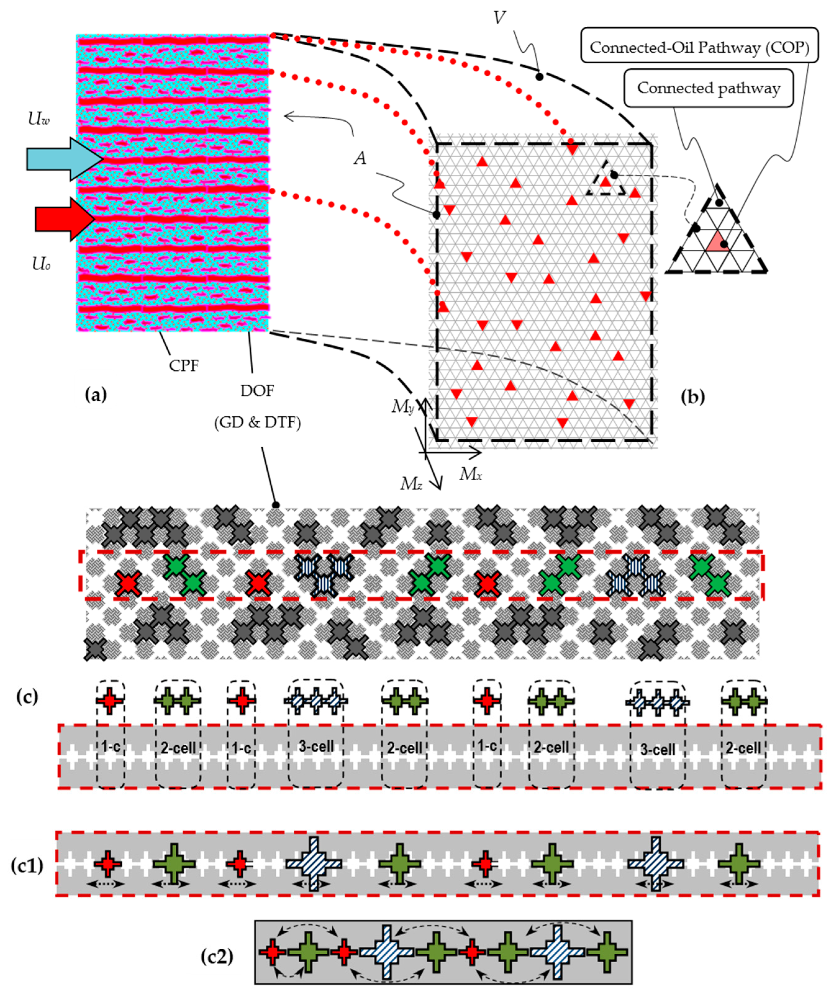
Figure 1.
(a) Schematic representation of the actual flow (left sketch) and its theoretical decomposition into prototype flows: Connected-oil Pathway Flow (CPF) and Disconnected-Oil Flow (DOF) (right sketch). (b) A microscopic scale representation (snapshot) of a DOF region. An oil ganglion of size class 5 is shown. For simplicity, all cells are shown identical and the lattice constant is shown expanded (chambers and throats have prescribed size distributions). The dashed, light grid lines define the network unit-cells. The thick dashed line separates the Ganglion Dynamics (GD) cells domain and the Drop-Traffic Flow (DTF) cells domain.
All types of flow have been observed experimentally in model porous media [
10,
20,
21] as well as in real porous media [
22,
23]. Each prototype flow has the essential characteristics of the corresponding flow pattern in suitably idealized form and so, the pore scale mechanisms are incorporated in the prototype flows.
In the Connected Pathway Flow (CPF) region the oil retains its connectivity and flows with virtually one-phase flow. The porous medium volume fraction occupied by the connected oil is denoted by β. The Disconnected-Oil Flow (DOF) regime is defined as the region composed of the rest of the unit-cells, so the associated volume fraction equals (1−β). This modeling decomposition is represented schematically by the right sketch in
Figure 1a, where the volumetric fractions of the prototype flows have been isolated and re-accounted over separate parts of the pore network reference volume,
V. A microscopic scale representation (a snapshot) of a typical DOF region is shown in
Figure 1b. An oil ganglion having a typical “cruising” configuration [
18] is shown at the center. All the cells that accommodate parts of this (or any other) oil ganglion are called ganglion cells and are demarcated with a thick dashed line. The rest of the cells in the DOF regions are cells containing water and oil drops. These cells comprise the regions of the Ganglion Dynamics (GD) and Drop Traffic Flow (DTF) domains respectively.
The fraction of all the ganglion cells over all the DOF region cells is denoted by ω, and is called the GD domain fraction. The DTF domain fraction in the DOF region equals (1−ω).
Sw, β and ω are called flow arrangement variables (FAV) because they provide a coarse indication of the structure (or “immiscible mixing”) of the flow pattern. One of the objectives of the DeProF model algorithm is to determine the values of Sw, β and ω that conform to the externally imposed flow conditions (Ca, r).
The flow analysis is carried out at two length scales, a macroscopic scale (10
12 pores, or more) and a microscopic scale, and produces a system of equations that includes macroscopic water and oil mass balances, flow arrangement relations at the macroscopic scale, equations expressing the consistency between the microscopic and macroscopic scale representations of these balances in the DOF region and an equation that is obtained by applying effective medium theory [
24] to the “equivalent one-phase flow” in the DOF (GD and DTF) region—implicitly representing the transfer function for this region [
18,
19]. The system is closed by imposing an appropriate type of (sharply decreasing) distribution function for the ganglion volumes, which is dictated by the physics of ganglion dynamics, in compliance with experimental observations [
20,
21] and numerical/pore network simulations [
25,
26]. In reality, large ganglia cannot survive because, as they migrate downstream the tortuous paths of the pore network, they break-up into smaller ones.
2.2. Physically Admissible Flow Configurations
A core feature of the DeProF model is the detection of all flow configurations that are physically admissible under the imposed macroscopic flow conditions. On a mesoscopic scale (say 104–109 pores), the actual flow at any given region of the porous medium “wanders” over the domain of physically admissible flow configurations “visiting” any one with equal probability or frequency (ergodicity).
To detect these flow configurations the domain {
Sw, β, ω} of all possible flow arrangement parameter values is partitioned using sufficiently fine steps to obtain a 3D grid (
Figure 2). Then, for each grid set of the flow arrangement parameters values (
Sw, β, ω), the
DeProF algorithm is asked to detect (if) a solution of the
DeProF equations (exists). In such case the selected set of (
Sw, β, ω) values, is allowed as a
physically admissible solution (PAS) and is denoted as (
Sw', β’, ω’). Otherwise, the set is rejected. In the end, the subdomain of the {
Sw, β, ω} space, denoted Ω
PAS, is detected as the set of physically admissible solutions.
The measure (“volume”) of Ω
PAS is given by:
Where Ω
PAS(
Ca,r) stands for integration carried over the physically admissible ranges in (
Sw, β, ω) for the imposed
Ca,
r values. The volume of Ω
PAS is a measure of the degrees of freedom of the process at the mesoscopic scale; it is also related to the rate of entropy production at the mesoscopic scale (configurational entropy).
By assuming that each physically admissible solution is visited with the same probability, or frequency (assumption of ergodicity), and averaging over their domain, Ω
PAS, a unique solution for the macroscopic flow is obtained. For any quantity, Φ’, the corresponding expected mean macroscopic flow quantity, Φ, is defined as:
Note, in Equation (3), a prime is used to denote physically admissible values of any quantity, Φ. Unprimed variables denote the expected, time-average value of that quantity.
As with any macroscopic physical quantity, unique set of values for (Sw, β, ω) can be obtained by averaging over the domain of physically admissible solutions, using Equation (3), with Φ replaced by Sw, β and ω. These values define the flow configuration of the mean macroscopic flow (ergodicity).
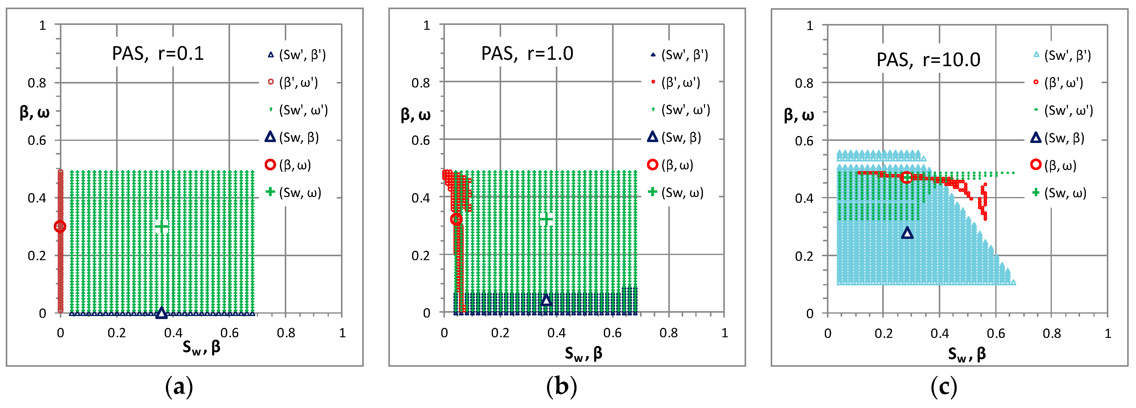
Figure 2.
Typical domains of physically admissible flow configurations, as predicted by DeProF model simulations. For any fixed, externally imposed, flow conditions, (Ca, r), the two-phase flow visits a canonical ensemble of physically admissible flow configurations (Sw', β’, ω’) depicted by the cloud of small, red balls. Here, Ca = 1.19 × 10⁻⁶, κ = 1.45 and flowrate ratio values, r, span 2 orders of magnitude. A unique set of values for (Sw, β, ω), the large, black ball, is obtained by averaging over the ensemble and defines the mass center of the red cloud. The shape and position of the red cloud changes with flow conditions.
In computational practice, the size of the domain of physically admissible solutions,
VΩPAS, as well as any expected mean macroscopic flow quantity, Φ, can be determined by any coarse graining (discretization) procedure used to detect the ensemble of physically admissible solutions and delineate its envelope. The phase space {
Sw × β × ω} pertaining to the FAVs, is partitioned in corresponding
NS ×
Nβ ×
Nω phase space voxels. The finer the graining, the smaller is the size of these voxels. Nevertheless, the smallest discretization size of voxels has a limit; it cannot become smaller than a minimum, critical size in each prototype flow. Suppose that we detect two solutions (
Sw', β’, ω’)
i and (
Sw', β’, ω’)
i+1 associated with two adjacent voxels,
i and
i+1. These solutions are virtual, in the sense that they have been detected by a numerical algorithm implementing a particular discretization. In essence they have been picked-up from the complete ensemble of the physically admissible solutions. So, there is a great chance that other flow configurations exist as well—other than those detected (as solutions) by the discretization scheme. This possibility could be verified by re-discretizing the phase space into a finer grid implementing smaller voxels. The new virtual ensemble of physically admissible solutions would eventually contain more solutions. Nevertheless, it would not occupy a volume in the FAV phase space larger than the previous ensemble (associated to the coarse grid). The only difference between the two virtual ensembles would be on the “texture” of their envelopes. The latter would have a finer surface than the former. We would be able to repeat the re-discretization with finer and finer grids, resulting in smaller and smaller voxels. But we would eventually reach a critical size whereby solutions would not have discernible characteristics. This limiting critical size (threshold) depends on the structure of the pore network (its fractal characteristics) and on the modeling of the prototype flows (the characteristic sizes of the disconnected fluidic elements). We will address this issue in
Section 4.
2.3. Discussion on Assumption of the Process Ergodicity
Assumption of ergodicity could be accounted for as “a best possible guess”. Nevertheless, there are strands of evidence supporting that the sought process could actually be treated as ergodic. Let us start by the empirical knowledge, acquired from laboratory studies. One may refer to the laboratory work of Avraam and Payatakes [
10], whereby immiscible steady-state flow configurations in glass pore network models have been studied. Snapshots as well as videos, capturing the phenomenon at the pore network model scale, show that interstitial flow arrangements and states of dynamic equilibrium are maintained. The system constantly and incessantly rearranges itself within a well defined phase space of configurations so long as the externally imposed flow conditions (flowrates of oil and water) are kept constant. If the externally imposed flow conditions change (to any other constant configuration), the system reorganizes itself into another steady-state, rearranging itself within another well defined configuration. This can be attested—to the level of available laboratory data—by observing the videos capturing different externally imposed flow conditions.
Moving into mechanistic modeling, the clouds of red balls in the diagrams of
Figure 2 is also an expression of self-organization. The driven system “reorganizes itself”, as expressed by the different shapes/positions of the cloud, to “fit” (or, to “survive” over) the externally imposed flow conditions. In essence, the red cloud is a manifestation of the self-organization of the virtual system, stemming from the
DeProF algorithm—implementing the
DeProF mechanistic model equations as well as the strategy in detecting the physically admissible flow configurations that satisfy the
DeProF equations. In the
DeProF mechanistic model, ergodicity comes into play when the cloud of physically admissible flow configurations (
Sw', β’, ω’), is replaced by the average macroscopic flow configuration (
Sw, β, ω), Equation (3). To test the specificity of the
DeProF model predictions, that are based on the underlying assumption of ergodicity, the average mechanical power dissipation,
W, estimated through Equation (3), was benchmarked against the available laboratory data. In these simulations, the
DeProF algorithm was implemented to account for the particular geometry of the pore network model. The comparison is depicted in the diagrams of
Figure 5 in [
12] (originally of
Figure 3 in [
19]). It is obvious that there is an excellent agreement between the
DeProF model predicted values and the values measured in the laboratory study.
A last point in considering the process as ergodic, and especially in considering that effective (or average or measurable) macroscopic physical quantities stem (with equal probability) from the entire set of all physically admissible interstitial flow arrangements, is the following argument: if it was the other way round, that is, if the case was that there are preferable flow arrangements (visited more frequently than others), then we would have to allow less degrees of freedom in the
DeProF model, risking to bias the theoretical analysis and drive the solution towards an erroneous (unphysical or biased) direction. To avert such a risk, Valavanides and Payatakes [
18,
19] decided to use a uniform distribution of probabilities as the given prior, for the process in taking all physically admissible configurations.
Moreover, from a probabilistic point of view, the
ergodicity of a system is based on the term “equal probability”, a term which goes back to the very foundations of probability (classical definition). The
classical definition of probability is essentially based on two assumptions, which seem to be its disadvantage. One of them is, that
each one of the possible results of a random experiment has the same possibility or
probability of happening. In practice it is difficult to determine equally likely results/events, the ability comes after long observation, experience and experimentation. That is why we say that this definition is a consequence of the
principle of insufficient reason (first enunciated by J. Bernoulli) [
27]: “
If we don’t have enough knowledge (evidence) to decide otherwise,
the results of a random experiment are assumed to be equally likely.” Still, the concept of “the equal possibility/probability” (equally likely events), used in the classical definition of probability is intuitive and cannot be based/strictly defined on/by pure mathematics. It is based somewhat on the very concept of probability that we are trying to define.
2.4. Statistical Thermodynamics Aspects of Two-Phase Flow in Pore Networks
Steady-state two-phase flow in porous media is an off-equilibrium process. One needs to provide energy to the process to keep it at fixed operating conditions,
i.e., to maintain its operation at fixed values of
Ca and
r (and at fixed temperature, say
T0). A justification of the existence of optimum operating conditions was recently proposed [
17] along the lines of the postulate stating that the efficiency of a stationary process in dynamic equilibrium is proportional to its spontaneity [
28]. Spontaneity, the notional inverse for irreversibility, may be quantitatively assessed by the amount of entropy produced globally. To evaluate the entropy, we need first to define the physical domains in which the process of steady-state two-phase flow in pore networks is maintained at dynamic equilibrium under fixed
Ca and
r.
With reference to
Figure 3, the
System comprises the porous medium and the two fluids. The
Surroundings are the heat reservoir in which the System resides and with which it exchanges heat at constant temperature, say
T0. The infinite heat reservoir can absorb all the heat released by the System. The
Universe comprises the System and the Surroundings.
The entropy produced globally (within the Universe),
SUNIV, is the sum of two terms: a term representing the entropy released from the System to the Surroundings,
SSUR, and a term representing the entropy produced within the System,
SSYS:
Each term denotes a source of entropy. The rate of entropy production in the Surroundings (maintained at constant temperature
T0),
SSUR, is due to the rate with which mechanical energy is dissipated within the System,
W = (
q0 +
qw) Δ
p, irreversibly transformed into heat,
Q =
W, a source of microscopic chaos, and then released to the Surroundings:
The second source of entropy,
SSYS, may be directly related to the multitude of the physically admissible flow configurations (the ensemble of physically admissible solutions) that are maintained for so long as the (steady-state) process is kept at conditions of dynamic equilibrium. It can be interpreted as the production of chaos over mesoscopic scales (configurational entropy). It can be expressed, similar to the Boltzmann entropy formulation in statistical mechanics, as:
where
kss2fpm is a constant quantity, similar to Boltzmann’s constant in the statistical thermodynamics definition of entropy, that would have to be appropriately defined for the sought process, (index “ss2fpm” stands for “steady-state 2-phase flow in porous media”), and
NPAS is the actual number of different mesoscopic flow arrangements (or microstates) consistent with the macroscopic flow at (
Ca,
r) conditions.
Figure 3.
The physical domains of steady-state two-phase flow in pore networks.
Figure 3.
The physical domains of steady-state two-phase flow in pore networks.
In order to maximize the efficiency of the process one should increase or even maximize the left side of Equation (4). Of the sum components, the first term represents the cost of energy irreversibly transformed into heat and released to the surroundings. Any increase of this term should be avoided; even better, this term should be decreased as much as possible. To do so, and, in parallel, increase as much as possible the total entropy in the Universe—in order to increase the efficiency of the process—one may arrange or even “force” the process to operate in such conditions for which the flow is optimally rich (but not necessarily richest) in different physically admissible flow arrangements.
Of the two entropy production terms the first, SSUR, is considered to be known (or given); it can be measured or it can be estimated if the DeProF, or any other model algorithm is implemented in the process analysis and the detection of the physically admissible flow configurations. The second term, SSYS, is not readily available. In the following, we will present the methodology for estimating, the number of microstates of the process for fixed macroscopic flow conditions, given the ensemble of physically admissible flow arrangements.
The objective of the aforementioned analysis is to examine if the maximum entropy production principle could be applied to the sought process (two-phase flow in porous media) and/or if it could provide a sound theoretical background for explaining (and understanding) why, in these processes, there exists a locus of optimum operating conditions and what are the critical characteristics of this locus. In particular, what makes some steady-states more “efficient” than others (in terms of specific cost of oil flowrate) and what are the critical characteristics that set-up the optimum operating conditions? The theoretical study presented by Niven [
29], on the convergence of dissipative flow-controlled systems towards steady-state positions and, in particular, the discussion therein, can provide the theoretical framework for establishing the MEP principle(s) for the sought process and address the aforementioned questions.
4. Definition and Counting of Microstates
The global (total) entropy production (pertaining to the System and its Surroundings—
Section 2) is considered to comprise two constituents, each evaluated over different size scales: thermal entropy is estimated over the continuum mechanics scale (thermodynamics), whereas configurational entropy is considered over a discrete (and countably finite) scale, whereby the microstates have been grouped together to obtain a countable set (statistical mechanics).
4.1. Countability of Process Microstates
In the system examined here, the pore network (the medium) comprises discrete classes of unit-cells, within which, discrete fluidic elements exchange momentum. A microstate is specified by the positions and momenta of all the fluidic elements—connected-oil pathways, ganglia and drop-traffic flow cells. Ganglia can only occupy countably-many unit-cells and their mass is considered as integer multiple of a conceptual elemental void space (CEVS, [
18]). Ganglion velocity is a function of its size and of the average flow conditions. It is classified on a one-to-one correspondence to the ganglion size. Only those ganglia belonging in the same size-class are considered to be mutually indistinguishable. Drop-traffic flow cells are identical (momentum-wise) since they contain water and uniformly dispersed oil droplets. Consider now a “virtual snapshot” of any physically admissible flow configuration, containing the positions and momenta of the fluidic elements. We count two microstates as different if the respective snapshots are different,
i.e., if the fluidic elements are arranged in different layouts. In essence, only their positions will be different. Since their velocity/momentum depend on their size and macroscopic flow conditions (uniform across all physically admissible arrangements), the velocity/momentum will be identical in all ganglia of the same class. Therefore, all ganglia are distinguishable by reference only to their size class. The aforementioned coarse-graining (pertaining to the size classes of network unit-cells and the size and velocity classes of fluidic elements) is inherent in the
DeProF model algorithm. Therefore, any counting of microstates in the present work will be fully consistent with the
DeProF model provisions.
For every set of externally imposed conditions (Ca, r) there corresponds a set of physically admissible arrangements of prototype flows, comprising a canonical ensemble. The ensemble is determined by values of the flow arrangement variables {Sw’, β’, ω’}, namely, the water saturation, Sw’, the volume fraction of connected pathway flow cells, β’, and the volume fraction of ganglion unit-cells within the disconnected oil flow unit-cells, ω’. Each one of these flow arrangements, described by any unique triple value {Sw’, β’, ω’} has a countable set of microstates (or degrees of freedom) that may be evaluated by combinatorial analysis.
In the following, we will focus on the estimation of the configurational (discrete scale) microstates stemming from the different arrangements of the fluidic elements for every physically admissible flow configuration. In particular, the number of microstates of the connected-oil pathways will be evaluated by considering an equivalent “balls-in-boxes” problem in combinatorial analysis (see
Section 4.2). The number of different microstates in the disconnected-oil flow will be evaluated by considering an equivalent “chains-in-barbs” problem in combinatorial analysis (see
Section 4.3). Then, considering that each problem is independent, the basic counting principle accounts the total number of microstates as the product of the individual numbers of microstates. Still, this would only account the microstates of
any-one physically admissible flow configuration. Passing to the next scale of hierarchic modeling, the canonical
ensemble of physically admissible flow configurations, the number of microstates will have to be enriched by the number of microstates corresponding to each one of the physically admissible solutions (see
Section 5).
4.2. Counting of the Connected Pathway Flow Microstates
Consider the reference volume comprising a total of
MxMyMz =
M unit-cells (
Section 3.1). Connected-Oil Pathways (COPs) occupy any β’ region of the pore network and remain aligned to the macroscopic flow. Of all the unit-cells in the reference volume, β’
MxMyMz = β’
M unit-cells are occupied by connected oil. Now, since Connected-Oil Pathways are aligned to the macroscopic flow, and they have an infinite length, or at least, long enough to be laid across the reference volume, volume fractions and area fractions are equal. COPs occupy β’
MxMy part of the frontal area (perpendicular to the macroscopic flow), see
Figure 5a,b. At any instance, each one of the COPs occupies a connected pathway of unit-cells but not necessarily the same. As time evolves, COPs may rearrange their tracks between parallel pathways. Since the process is considered to be ergodic, during a large time frame, COPs may occupy any of the available connected pathways with equal probability. In that context the flow may take a number of different and equi-probable microstates. The problem of counting the CPF microstates is equivalent to the problem of counting the number of different ways in placing a number of indistinguishable balls (the COPs) in a larger number of distinguishable boxes (the pathways) with exclusion. The pathways are distinguishable because they provide the reference framework for comparing two instants (snapshots) of COP arrangements. Exclusion means that no identical snapshots of COP arrangements can be counted more than once.
Figure 5.
(a) Side view of the macroscopic flow comprising a mixture of connected and disconnected prototype flows; (b) Frontal, microstate snapshot of the connected-oil pathway flow (CPF); (c) Side, microstate snapshot of the Disconnected-Oil Flow (DOF); Focus is on the middle-row, colored ganglia. (c1) & (c2) Separation into two complementary problems in combinatorial analysis. Microstate snapshot of repositioning of ganglia (c1) for a possible permutation (c2) (a 1-2-1-3-2-1-2-3-2 snapshot).
Considering that the frontal area of the reference volume comprise
K =
MxMy unit-cells or pathways, then, for any physically admissible flow arrangement,
NCOP = β’
K of the pathways are occupied by indistinguishable connected-oil pathways that may take any possible arrangement parallel to the macroscopic flow (recall that
K is the number of the pore network virtual pathways),
Figure 5b. Combinatorial analysis provides the solution to this particular “balls-in-boxes” problem. The number,
PCPF, of different ways (excluding double counting of two identical arrangements) in placing
NCOP indistinguishable balls (the connected-oil pathways) into
K distinguishable boxes (the pore network virtual pathways), is given by:
4.3. Counting of the Disconnected Oil Flow Microstates
We must also count the number of different ways that a population of ganglia of various sizes (i.e., of a given size distribution) may be arranged to occupy the available pore network unit-cells. The question is equivalent to how many different ways a variety of short-length chains (ganglia), each one of size ranging from 1 to Imax links (the ganglia), may engage onto an available number of barbs (the ganglia fitting into the available unit-cells).
Every physically admissible flow arrangement, comprises a reduced ganglion size distribution, {; i=1, 2, …, Imax}, i.e., a population density distribution of an integer multiple of i-linked ganglion unit-cells (oil saturated unit-cells). Ganglia of different size classes may arrange themselves anywhere within the (1−β’) volume fraction of the pore network unit-cells comprising the Disconnected-Oil Flow (DOF) domain.
The ganglion unit-cells may be considered as “links” being used to construct “chains” of different sizes,
i.e., ganglia of different sizes, with their size ranging from 1 to a certain number
Imax. Given the ganglion size distribution, the distribution of the population of
i-size ganglia within the reference volume, is directly derived from Equation (7) as:
with
n1,
n2,
Imax and ζ given (better, determined as a physically admissible solution, e.g., implementing the
DeProF model algorithm) and 0 < ζ < 1, e.g., ζ ∈ {0.3, 0.5, 0.7} and (
Imax <<
Mz).
The total number of chains (of all sizes),
NC, the total number of links in these chains (ganglion unit-cells),
NGUC, and the total number of Drop Traffic Flow (DTF) unit-cells,
NDTF, are given respectively by the following expressions:
In this context, there are M(1−β’) unit-cells available for hosting the Disconnected-Oil Flow (DOF) cells. These comprise NGUC unit-cells saturated with oil (ganglia cells) and NDTF unit-cells containing water and oil droplets. Obviously, NGUC + NDTF = M(1−β’).
Ganglia of the same size class are indistinguishable, whereas ganglion classes are—by definition—distinguishable (based on their size, i). Network unit-cells are distinguishable because, as previously stated, they provide the reference framework for comparing two instances (snapshots) of ganglion arrangements in DOF. There is no restriction in ordering the ganglia. The only requirement is that all ganglia are parallel to the z-direction (of the macroscopic flow). Therefore, the network unit-cells available for DOF (= GD + DTF) can be virtually (re-)ordered (aligned) in just a single row of size M(1−β) = NGUC + NDTF.
The problem of counting the different number of ways that ganglia unit-cells may be arranged within the DOF unit-cells is separated in two parts. In the 1st part, we find the number of ways we can choose
NC empty cells from a total of
NDTF+
NC cells. This is a problem of repositioning
NC balls in (
NDTF +
NC) cells. In the 2nd part, we find the number of permutations (ordering) of the
NC ganglia. Then, by applying the so called “basic counting principle” [
30], we derive the result by multiplying these two numbers.
1st part: The problem of placing a chain of size
i, in empty unit-cells, each one containing one link, is equivalent to replacing the
i empty unit-cells with one single cell (“i-cell”) and then place these
i links (the "i-chain") in this “i-cell”, (
Figure 5c,c1). In the reference volume, we have
NDTF empty unit-cells plus
NC empty i-cells (of various
i sizes) and we have to place, in these cells,
NC chains (of various i-chain sizes) in such a way that each i-cell can contain at most one i-chain (
Figure 5c1) . Since the
NC i-cells are identical, the number of ways we can place
NC i-cells in a total of
NDTF +
NC cells (order does not matter) is equal to:
2nd part: There are
N1 chains of size 1,
N2 chains of size 2 and so on,
NImax chains of size
Imax. In other words, there are
NC objects, grouped in
N1 indistinguishable objects,
N2 indistinguishable objects and so on, up to
NImax indistinguishable objects. These needs to be placed in corresponding
NC receptors, considering no receptor is to contain more than one object. We seek the number of different permutations in allocating the
NC objects in the
NC receptors,
Figure 5(c2). This problem can be tackled as the classical problem of estimating the number of different permutations,
PD2’ of
NC objects (ganglia), of which
N1 are alike,
N2 are alike, …,
NImax are alike [
30]. This is equal to:
Combination of 1st & 2nd part: By implementing the basic counting principle [
30], the number of ways of placing the
NC chains in the
NDTF+
NC empty hooks (barbs) or, equivalently, the number of different ways that the given population of ganglia may be arranged to occupy the available empty network unit-cells,
PDOF’, is equal to the multiplication of
PD1’ by
PD2’:
Example: Focusing on the paradigm of
Figure 5, and specifically on the array delineated with the dashed-line box, we count
NC = 9 ganglia (chains) of different size (i-cells), with
NGUC = 1 + 2 + 1 + 3 + 2 + 3 + 2 + 1 + 2 = 17 links. There are
NEUC =
NDTF +
NGUC = 40 empty unit-cells available for hosting these links (receptor cells),
Figure 5c. Of the
NEUC cells,
NGUC will be occupied whereas
NDTF = 23 unit-cells will be available for repositioning the chains. Therefore the number of different positioning of the particular array of nine chains (i-cells) within a total of 32 receptors (nine i-cells and 23 unit-cells),
Figure 5c1, is equal to
PD1’ = (23+9)!/(9! × 23!) = 32!/(9! × 23!) = 28,048,800.
Next we have to count how many times we may reorder the array of the
NC = 9chains (chains of the same size are indistinguishable). This problem is equivalent to the problem of estimating the number of times we can reorder a group of
NC = 9 balls comprising
N1 = 3 red balls,
N2 = 4 green balls and
N3 = 2 blue balls (
Figure 5c2). This number is equal to
PD2’ = 9!/(3! × 4! × 2!) = 1,260. Therefore, the number of different microstates of the array in
Figure 5c is estimated at
PDOF’ =
PD1’
PD2’ = 28,048,800 × 1260 = 35,341,488,000.
4.4. Counting of Microstates per Physically Admissible Solution
Implementing once more the basic counting principle [
30], the number of different microstates,
P’, pertaining to a physically admissible prototype flow arrangement determined by the triplet of flow arrangement variables (
Sw', β’, ω’) is given by:
Now, considering the structure of expression Equation (16), its computation would require excessive computational resources even for a small pore network. Recall the 109 microstates that we computed in the disconnected oil flow taking place within just a small strip of 40 cells. Nevertheless, we do not have to actually compute such large figures. We only need to estimate the natural logarithm of expression Equation (16) and use it in the Boltzmann type expression, Equation (6). Therefore instead of direct computation of P’, it is possible to tackle its natural logarithm, lnP’.
Then, implementing the “Stirling approximation limiting procedure” formula:
The equality being true in the sense that
and
are almost identical, results:
Now, replacing
NCOP = β
’K, and using expressions Equations (9)–(12) yields (by straightforward algebra) a form similar to the Boltzmann–Gibbs entropy [
31] expression:
Note that in Equation (20) there are two contributions in the number of microstates:
- (a)
The extensive contribution of the size of the reference frame (volume and frontal area), expressed by the values of “user-selected” parameters M and K respectively. Their value depend on the aspect ratio of the reference volume and the type of the pore network. For the sought network, considering a cube as reference volume, parameters K and M are related as . For a lattice constant, 1.221 mm, K = 4.699631 × 10⁻³.
- (b)
The non-extensive contribution of the actual flow configuration, expressed by reduced variables, namely the flow arrangement variables β’, ω’ and the reduced ganglion size distribution, n’i, i = 1, …, Imax.
Recalling Equation (16), Equation (20) can be recast as:
where, by using once more Equation (18) and straightforward algebra, it is easy to verify that:
represents the number of microstates of the connected-oil pathway flow (CPF), see Equation (8), and
represents the number of microstates of the Disconnected-Oil Flow (DOF), see Equation (15), which, on its merit, is expressed as the sum of two terms,
pertaining to the repositions (D1) and the permutations (D2) of ganglia in the DOF domain.
Expressions (20) and (21) comprise two terms and each can be interpreted as follows: there are two domains within the pore network where microstates “live”: the reference area perpendicular to the flow (frontal area) and the reference volume. The reference area is occupied by two complementary entities, connected-oil pathways that may arrange over any β’ fraction of it and DOF pathways that may arrange over the complementary fraction, (1−β’). The corresponding microstates are given by the first term in Equation (20), or in Equation (22), as two separate Boltzmann–Gibbs (B-G) expressions, (−β’lnβ’) and (−(1−β’)ln(1−β’)). It is similar to the expression describing the microstates of an (immiscible) mixture of molecules of two (chemically inert) gases, sharing complementary volume fractions within a container [
31,
32].
The other microstate domain comprises the (1−β’) volume fraction of the pore network that is shared by two entities: the Drop Traffic Flow (DTF) unit-cells, having identical size, and the ganglia unit-cells, having a size distribution. The corresponding microstates are given by the second term in Equation (20) (or in Equation (23)) again as a sum of two separate Boltzmann–Gibbs (B-G) expressions. The DTF unit-cells are free to take any placement within the (1−ω’)(1−β’)fraction of the reference volume, hence the expression (1−β’)(−(1−ω’)ln(1−ω’)). The ganglia unit-cells “live” within the complementary domain, ω'(1−β'). If they would have been all singlets, i.e., of size 1, they would be occupying the complementary domain ω’(1−β’) described by the B-G term, (−ω’lnω’). Nevertheless, this case—ganglia singlets—is very particular. In general, ganglia comprise an (immiscible) mixture of groups (classes) of different size, each represented by its own B-G expression, (−ni’ lnni’), mutually excluding each other from fully occupying the available ω’(1−β’) domain. In other words, if all ganglia were exclusively and equally partitioned into singlets, then the number of microstates would equal (−ω'lnω'); nevertheless this number is actually reduced by the accumulated number of microstates of ganglia of size i, (−ni’ lnni’), for i=1 to Imax. This complementarity is expressed by the B-G expression, , in the second term of Equations (20) and (25).
5. Configurational Entropy
To proceed with the computation of the configurational entropy of the process for any particular macrostate flow condition (Ca, r), or macrostate configurational entropy, SSYS(Ca, r), we need first to estimate the number of microstates of the canonical ensemble of physically admissible solutions, P(Ca,r).
We implement the basic counting principle for the microstates pertaining to each one of the physically admissible solutions,
Pj’, for
j∈{1, …,
NPAS(
Ca, r)}:
and reduce the computational burden by tackling its logarithm:
Then, the macrostate configurational entropy of the process can be expressed as:
Alternatively, the macrostate configurational entropy of the process can be expressed as the sum of the configurational entropies of the physically admissible solutions,
S’
SYS,j, for
j∈{1,…,
NPAS}. This is justified by considering that, essentially, configurational entropy provides an appropriately reduced measure of the process’ degrees of freedom. The term “appropriately reduced” refers to the Boltzmann type constant for the particular process,
kDeProF. So long as any two flow configurations (members of the ensemble of physically admissible solutions) are discernibly different, their unified degrees of freedom add. In addition, since any two different flow configurations have the same physical structure, they share the same constant,
kDeProF. Therefore we may write:
Obviously, the two expressions Equations (28) and (29) are identical.
In this context, the contribution of microstates within each physically admissible flow arrangement, Pj', as well as the contribution of other microstates stemming from the plurality of all physically admissible flow arrangements, NPAS(Ca,r), have all been taken into account.
An open problem that still needs to be addressed is the delivery of an expression for the constant kDeProF appearing in the expressions of Equations (28) and (29). Actually the kDeProF constant must have an effective character, in the sense that it must blend the contributions of two types of microstates, Equation (21), extending over different domains. In specific, the connected-oil pathway (CPF) microstates, Equation (22), extending over a reference surface (frontal area), and the Disconnected-Oil Flow (DOF) microstates, Equations (23)–(25), extending over a reference volume.
The associated configurational entropies must be expressed using specific, Boltzmann-type constants, say
kCPF and
kDOF, because of the different energy density associated with each prototype flow. Then, taking into account Equation (21), the Boltzmann-Gibbs expression for the configurational entropy should be expressed as:
6. Results and Discussion
To materialize the expressions delivered in
Section 4 we have made indicative calculations of the number of microstates for various flow configurations. The flow configurations have been chosen from the ensemble of physically admissible solutions obtained from
DeProF model simulations for macroscopic flow conditions, (
Ca, r), pertaining to combinations of typical capillary number,
Ca = 1.0 × 10
−6, and flowrate ratio values,
r = 0.1, 1.0 and 10.0, within a 3D model pore network and for fluid systems with a typical oil/water viscosity ratio, κ = 1.45. The specific geometrical characteristics of the network as well as the physicochemical characteristics of fluids are presented in the
Appendix. The ensembles of physically admissible solutions, corresponding to the above flow conditions are presented in the diagrams of
Figure 6. The projections of the cloud of all detected solutions, over the (
Sw × β), (
Sw × ω), (β × ω) planes of the FAV phase space are depicted with small markers. The projections of the average flow configuration (
Sw, β, ω) are identified with large markers.
Figure 6.
Projections of the domain of physically admissible flow configurations, (Sw', β’, ω’), and of the average, macroscopic flow configuration, (Sw, β, ω), for three different macroscopic flow conditions, pertaining to same capillary number value, Ca = 1.0 × 10⁻⁶ and to flowrate values (a) r = 0.1 (b) r = 1.0 and (c) r = 10.0. In every ordered pair of values, (x,y), x is the abcissa and y the ordinate.
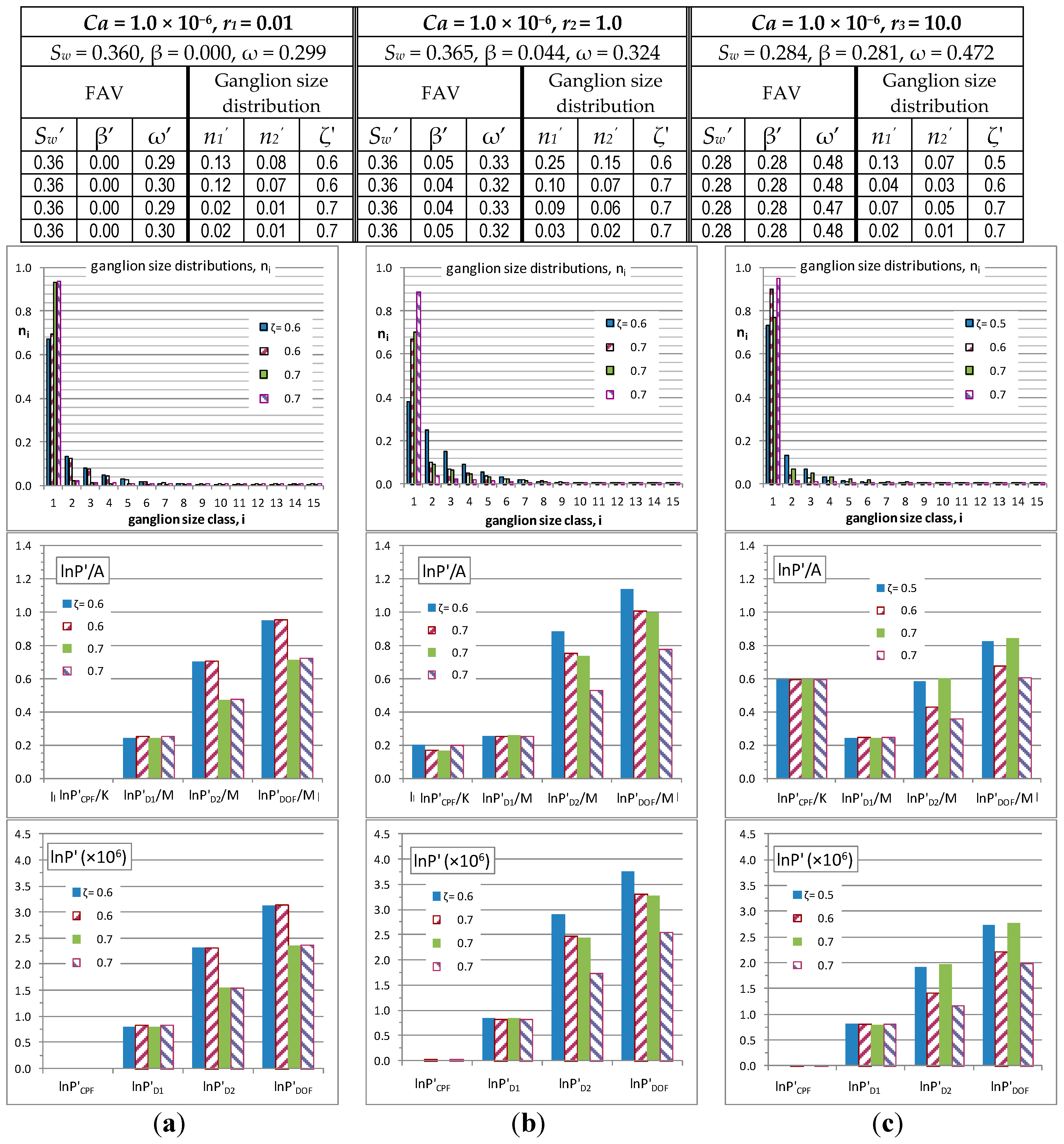
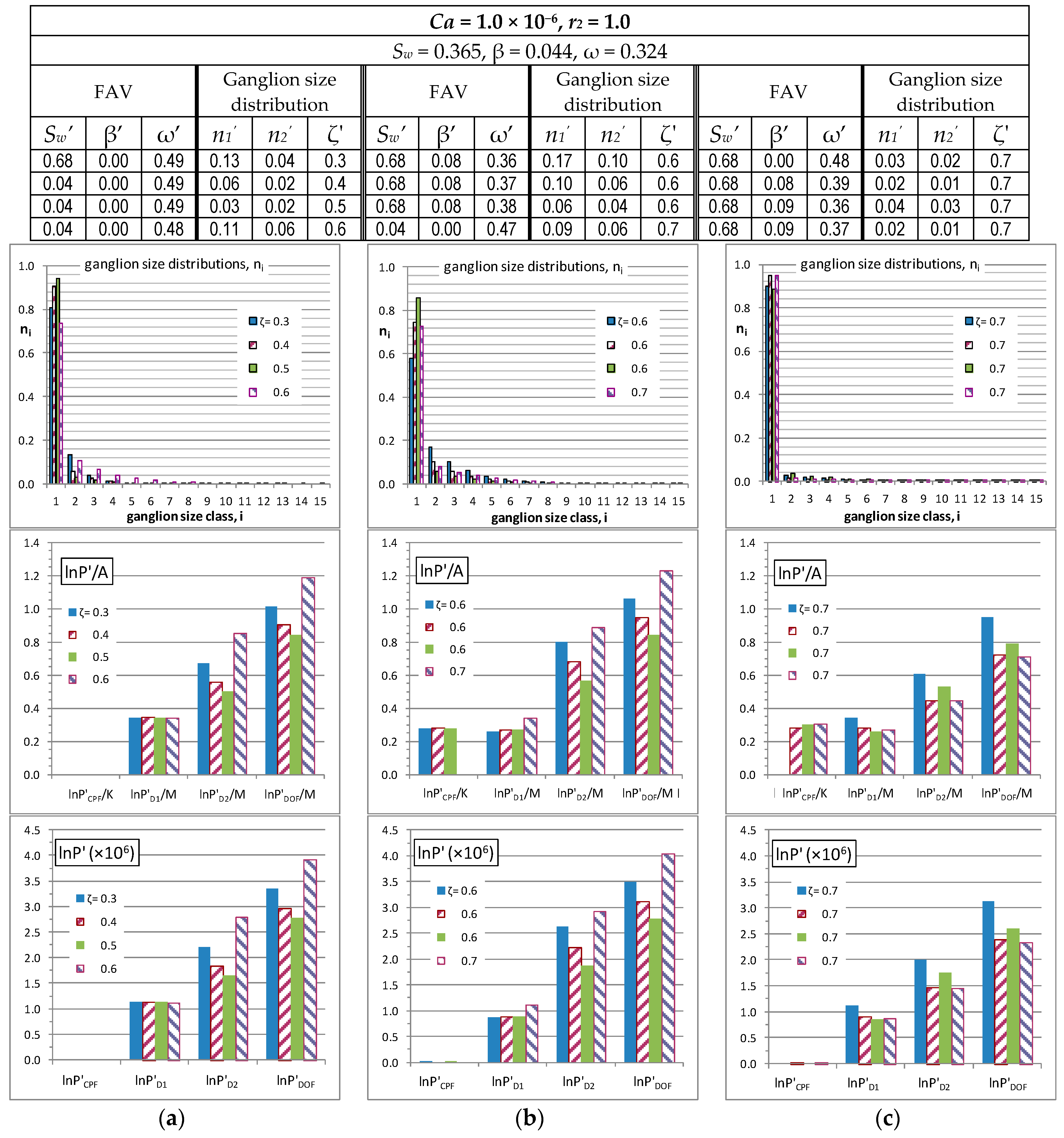
We have also designed diagrams (
Figure 7 and
Figure 8) to indicate the effect of the flow arrangement variables, (
Sw', β’, ω’), and the associated ganglion size distributions parameters, (
n1,
n2, ζ), on the number of microstates as well as on the relative and absolute contributions of the CPF and Disconnected-Oil Flow (DOF) microstates,
PCPF’ and
PDOF’. For that purpose, we have elected to show the microstates for two types of physically admissible flow arrangements and different sets of macroscopic flow conditions, (
Ca, r). “Moderate” flow arrangements are characterized by flow arrangement values (
Sw’, β’, ω’)close to the ensemble average, (
Sw, β, ω) and are presented in
Figure 7. “Extreme” flow arrangements are characterized by flow arrangement values (
Sw’, β’, ω’) pertaining to the extreme borderline corners of the ensemble envelope, and are presented in
Figure 8.
Referring to
Figure 7 and
Figure 8, the tabulated data at the top indicate values of the flow arrangement variables (FAV), (
Sw’, β’, ω’), and of the critical parameters, (
n1,
n2, ζ), that define ganglion size distributions,
ni, Equation (7). Each row pertains to one physically admissible configuration. The data from each row are used as input to corresponding expressions estimating the values of the physical quantities plotted in the diagrams.
The diagrams on the top row of
Figure 7 and
Figure 8 present the ganglion size distributions,
ni, corresponding to the examined physically admissible flow arrangements. The distributions have been determined directly from the associated tabulated data using Equation (7). The diagrams on the middle row present the non-extensive, reduced entropy contributions of the CPF and DOF prototype flows, as computed from Equations (22) and (23)–(25). The contributions of repositions (D
1), Equation (24), and permutations (D
2), Equation (25), of ganglia in DOF are also presented in the same diagrams. Similarly, the diagrams at the bottom row present the extensive, reduced entropy contributions of the CPF and DOF prototype flows (as well as the D
1 D
2 contributions).
Figure 7.
Diagrams of the ganglion size distributions (2nd row), the non-extensive (3rd row) and the extensive (4th row) reduced entropy contributions of moderate physically admissible flows for different macroscopic flow conditions, columns (a), (b), (c). Tabulated data indicate values of the flow arrangement variables, (Sw’, β’, ω’) and the corresponding parameters, (n1’, n2’, ζ’) of ganglion size distributions. In the ordinate titles of the 3rd and 4th row diagrams, P’ denotes any of the PCPF’, PD1’, PD2’, PDOF’ contributions, whereas "A" in denominator denotes either K or M.
Figure 8.
Diagrams of the ganglion size distributions (2nd row), the non-extensive (3rd row) and the extensive (4th row) reduced entropy contributions of extreme physically admissible flows for same macroscopic flow conditions. Tabulated data indicate values of the flow arrangement variables, (Sw’, β’, ω’) and the corresponding parameters, (n1', n2', ζ') of ganglion size distributions. In the ordinate titles of the 3rd and 4th row diagrams, P’ denotes any of the PCPF', PD1', PD2', PDOF' contributions, whereas "A" in denominator denotes either K or M.
All diagrams in
Figure 7 and
Figure 8 pertain to flow configurations selected from the ensemble of physically admissible configurations consistent with 3 different sets of macroscopic flow conditions, (
Ca, r). The examined macroscopic flows share the same capillary number value,
Ca = 1.0 × 10
−6. The diagrams in
Figure 7 pertain to flowrate ratio values,
r = 0.10,
r = 1 and
r = 10.0, in corresponding columns (a), (b) and (c). In each column, the flow arrangement values, (
Sw’, β’, ω’) are selected in proximity to the corresponding average, macroscopic flow arrangement, (
Sw’, β’, ω’). The diagrams in
Figure 8 share a common value for the flowrate ratio,
r = 1 ; diagrams in columns (a), (b) and (c) correspond to extreme physically admissible flow configurations,
i.e., the flow arrangement variables (FAV) are as distant as possible from the FAV of the physically admissible ensemble average.
The diagrams in
Figure 7 and
Figure 8 have been plotted for particular (moderate and extreme) flow configurations (as predicted by the
DeProF model algorithm) and, in that context, they exhibit an overview of the provisions of Equations (20)–(25) over the domain of physically admissible solutions. An interesting observation is the following.
The reposition of ganglia (D1), is insensitive to flow conditions (
Figure 7) and/or flow configurations (
Figure 7 and
Figure 8). Nevertheless, the ganglia permutations (D2) have a strong impact on the Disconnected-Oil Flow (DOF) microstates. This is mainly attributed on the term
, appearing in Equation (20), or in Equation (25). As expected, the number of ganglia permutations increases as ganglion size distributions extend over a broader size domain. On the contrary, a narrow ganglion size distribution reduces the number of ganglia permutations. This can be observed by comparing the diagrams in columns (a), (b) and (c),
Figure 7. As the ganglion size distributions—associated with the different flow configurations—become narrower (in the order (b)-(a)-(c)), the corresponding D2 contributions are progressively reduced. The physical explanation is the following. D1 is directly related to β’ and ω’, see Equation (24), which are macroscopic variables, in the sense that they contain average information (on volume fractions,
extending over the whole network) and indicate the
superficial structure of the flow. In contrast, D2 is directly related to the
interstitial structure of the fluidic elements,
i.e., the size distribution of Ganglion Dynamics (GD) cells and Drop Traffic flow (DTF) cells, Equation (25). Now, the same amount of oil can be allocated over different ganglia distributions, all of which have equal first moments (equal oil masses). Nevertheless, distributions with equal first moments may have significant differences over their higher class moments. In our case this is expressed by the ζ value, regulating the sharpness of each distribution and, because of mass balance normalization, its breadth, see columns (a), (b) and (c) in
Figure 7. And this, on its merit, has a significant impact on the number of permutations of the ganglia unit-cells (D2).
Could the analysis (presented in
Section 4 and
Section 5) be constructed directly from the independent variables—without relying on micro-scale modeling? The authors’ perception is that micro-scale modeling could not/should not be avoided. It could only be made simpler, only if it would not wipe-out or suppress the essential characteristics of the process. Considering the process to comprise exclusively the flow of two immiscible fluids (no reactions or mixing between phases), a microstate is determined as any internal flow configuration of the process, described by the triplet values (
Sw', β’, ω’) that are compatible with the externally imposed flow conditions, determined by the values of the independent variables,
i.e., the superficial velocities of oil and water,
Uo,
Uw, or, equivalently expressed in reduced form, by the capillary number,
Ca, and the flowrate ratio,
r. The triplet values (
Sw’, β’, ω’) describe the partitioning of the total flow into volume fractions of prototype flows. Of these three variables,
Sw' and β', pertain to prototype flow configurations that have no particular interstitial structure in the sense that no additional/detailed description at the pore scale is required. In contrast, ω' pertains to the volume fraction of Ganglion Dynamics, a prototype flow configuration that has a characteristic interstitial structure, stemming from the different ganglion size distributions. The latter must satisfy the micro- to macro- scale consistency equations for mass and flowrate of oil. And this is because the flowrate in each flow domain is related to (depends on) the macroscopic pressure gradient,
i.e., the solution. A simplistic approach would be to deprive ganglia velocity of their actual dependence on the locally induced macroscopic pressure gradient. But this would not only violate basic modeling principles in fluid mechanics (considering bulk viscosity and capillary hysteresis phenomena have a significant contribution), it would also not be consistent with the basic phenomenology of ganglion migration downstream the pore network—whereby migration velocity depends on the locally induced pressure gradient. Considering that disconnected oil remains stranded (immobile), provides an—optional—oversimplifying modeling approach, suggesting water saturation,
Sw, is to be considered as the independent variable of the process. Yet, this “conventional wisdom” fails to provide a rational explanation of the process phenomenology when disconnected-oil flow is substantial. And still today, the true/accurate description of the phenomenon relays to the classical Darcy fractional flow representation of the cause-effect relation (pressure gradient
vs. flowrates)
only if laboratory measured values of relative permeability to oil and water are provided,
i.e., an entirely phenomenological approach. The delivery and use of relative permeability diagrams implementing saturation as the independent variable is only conventional. Another overly simplistic situation where there is no flow of oil based on Ganglion Dynamics is—according to numerous laboratory studies—physically impossible if conditions of simultaneous flow of oil and water are to be maintained.
Returning to the question of the previous paragraph, the analysis could be constructed directly only if all of the oil would be disconnected in singlets (ganglia of uniform size 1)—a quite extraordinary situation. In that case, the dependence of the ganglion velocity on the solution (the locally induced macroscopic pressure gradient) would be uniform across all ganglia and there would be no need for a detailed microscopic representation of the flow (in terms of ganglion size velocity distribution), and micro- to macro- scale flow consistency equations would be easily satisfied without delving into microscopic scale dynamics. This case has been already addressed in the last paragraphs of
Section 4.
Another issue that needs to be addressed is how the structure of the virtual 3D pore network lattice relates to the presented methodology. The statistical treatment for any type of network lattice will be the same. A different type of pore network lattice/geometry (e.g., hexagonal close packed or face-centered cubic configurations, or lab-on-a-chip configurations) would allow different interstitial flow arrangements, therefore it would affect the non-extensive part of expressions, Equation (20). Comparative
DeProF simulations between 2D and 3D networks have been carried in the past with only quantitative differences [
33]. Accordingly, differences in the lattice size/structure (topology) would have a considerable effect on the extensive part,
M and
K, since the number of unit-cells per pore network volume (the lattice density of the network) would change.


