Stability Analysis and Synchronization for a Class of Fractional-Order Neural Networks

Abstract

Stability of a class of fractional-order neural networks (FONNs) is analyzed in this paper. First, two sufficient conditions for convergence of the solution for such systems are obtained by utilizing Gronwall–Bellman lemma and Laplace transform technique. Then, according to the fractional-order Lyapunov second method and linear feedback control, the synchronization problem between two fractional-order chaotic neural networks is investigated. Finally, several numerical examples are presented to justify the feasibility of the proposed methods.

1. Introduction

Neural networks have been put more and more attention up to now [1,2,3,4]. Ranging from combinatorial optimization, pattern recognition, associative memories and many other fields, neural networks have been successfully used. Fractional-order models can be well used to describe the hereditary and memory properties of many materials and processes compared with the conventional integer-order model [5,6,7,8,9]. The uniform stability of fractional-order neural networks (FONNs) with delay is studied in [10]. Literature [11] discusses the synchronization problem for the uncertain fractional-order chaotic systems by means of adaptive fuzzy control. The fractional-order expression of neural network models is also introduced to investigate biological neurons. The reasons rely on two main aspects, one is the fractional-order parameter that enlarges the system performance by heightening one degree of freedom, the other is its infinite memory. FONNs may be expected to provide an excellent instrument in the field of parameter estimation. Furthermore, it has been shown that neural networks approximation taken at the fractional level usually leads to higher rates of approximation . Taking into consideration these facts, it is easy to know that combining an infinite memory term into the model of neural network is a big development, and it is advisable to research FONNs.

Nowadays, the dynamics analysis of FONNs has become a very attractive research topic, and some important results have been given. For example, bifurcations and chaos phenomenon in FONNs are studied in [12,13,14]. In [15], energy-like functions are utilized to study the stability of FONNs. Mittag–Leffler stability for memristor-based FONNs is showed in [16]. Furthermore, [4] and [10] research the properties of the solution of FONNs, and some interesting results are obtained.

Stability analysis is a basic topic in system (fractional-order or integer-order) and control theory [17,18,19,20,21]. In [22], the exponential stability of high-order neural networks with proportional delay is investigated by using the Lyapunov method and matrix measure. Based on the nonsmooth analysis theory, multistability of memristive Cohen–Grossberg neural networks with non-monotonic piecewise linear activation functions and time-varying delays is obtained in [23]. The stability for fractional-order linear systems was firstly reported by Matignon in [24]. Then, the linear matrix inequality (LMI) technique for the stability region are presented in [25]. In [26], the Mittag–Leffler stability of fractional-order gene regulatory can be obtained based on the fractional Lyapunov method. The problem of stability analysis of fractional-order complex-valued Hopfield neural networks with time delays are considered in [27]. In addition, there are also some presented results which can be utilized to fractional-order linear systems. As discussed in [21,28], how to analyze the stability of fractional-order nonlinear systems is still not well investigated and requires further study. It is known that FONN have special form, so the stability condition may be simpler. There are some stability theories about the traditional neural networks. Most of these results are driven by choosing appropriate Lyapunov functions, but these methods can’t be extended into FONN directly. For example, in [29], α-stability for FONN is discussed, unfortunately, the given result is not correct [30]. So, it is necessary to obtained stability conditions for FONN.

The synchronization problem of neural networks has been widely discussed due to its potential applications in signal processing and combinatorial optimization, etc. Based on the LaSalle invariant principle and adaptive feedback control technique, the synchronization in an array of linear coupled neural networks with reaction diffusion is discussed in [31]. In [32], the projective synchronization for chaotic time-delayed neural networks is investigated by using the sliding mode control approach. By adding different intermittent controllers, the synchronization for neural networks with stochastic noise perturbations is studied in [33]. Reference [34] discusses anti-synchronization of a class of chaotic memristive neural networks with time-varying delays. For many, results involving synchronization of chaotic neural networks have been obtained [7,16,35].

To the best of our knowledge, dynamical properties of FONN can be rarely found in related literature. Based on aforementioned observations, stability analysis and synchronization of FONN are investigated in this paper. There are three main innovations are worth being emphasized:

• By utilizing Laplace transform techniques, The boundness and convergence of solution for FONN are investigated.
• A linear controller is designed for synchronizing fractional chaotic networks. Integration of the sign function is utilized in our control methods, so chattering phenomenon can be avoided.
• A simple auxiliary function is constructed, which may be helpful for stability analysis of fractional-order systems.

The remainder of this work is as follows: In Section 2, we give a mathematical model of FONN and some preliminaries for this work are needed. In Section 3, we drive two sufficient conditions, which are used to analyze the stability of FONN. Simulations are carried out in Section 4 to demonstrate theoretical analysis. Finally, Section 5 concludes this work.

2. Preliminaries

We will give some related results for fractional differential and integral formulas. For more details, one can refer to [36]. Firstly, the fractional-order integral is expressed as

$${}_0{D}_t^{-\alpha }x\left(t\right)=\frac{1}{\Gamma \left(\alpha \right)}{\int }_0^t\frac{x\left(u\right)}{{(t-u)}^{1-\alpha }}du.$$

(1)

where $0<\alpha \le 1$. In general, fractional-order derivative has three different definitions: G-L, R-L, and Caputo [36]. In this work, let us use Caputo’s derivative. In addition, it is defined as

$${}_0^C{D}_t^{\alpha }x\left(t\right)=\frac{1}{\Gamma (k-\alpha )}{\int }_0^t\frac{x^{\left(k\right)}\left(u\right)}{{(t-u)}^{\alpha -k+1}}du,$$

(2)

where $k-1\le \alpha <k$. Obviously, the Laplace transform of (2) is

$${\int }_0^{\infty }{e}^{-st}{}_0^C{D}_t^{\alpha }x\left(t\right)dt=s^{\alpha }X\left(s\right)-\sum _{j=0}^{k-1}{s}^{\alpha -j-1}{x}^{\left(j\right)}\left(0\right).$$

(3)

The definition of Mittag–Leffler function is given as [36]:

$$E_{\alpha ,\gamma }\left(\zeta \right)=\sum _{j=0}^{\infty }\frac{{\zeta }^j}{\Gamma (\alpha j+\gamma )},$$

(4)

where $\alpha ,\gamma >0$ and $\zeta \in C$. In particular, $E_{1,1}\left(\zeta \right)=e^{\zeta }$. According to [36], we have

$$\mathcal{L}\left\{t^{\gamma -1}{E}_{\alpha ,\gamma }(-a{t}^{\alpha })\right\}=\frac{s^{\alpha -\gamma }}{s^{\alpha }+a}.$$

(5)

Lemma 1.

[37]. If $A\in R^{n\times n},0<\alpha \le 1$, γ is a real constant, and $\varpi \in R^{+}$, then

$$E_{\alpha ,\gamma }\left(A\right)\le \frac{\varpi }{1+\parallel A\parallel },$$

(6)

where μ satisfies i) $\mu \le |arg(\mathrm{eig}\left(A\right)\left)\right|\le \pi$ and ii) $\pi \alpha /2<\mu <min\{\pi ,\pi \alpha \}$.

Lemma 2.

[19]. Let $0\le t\le T$ and

$$h\left(t\right)\le g\left(t\right)+{\int }_0^{t}m\left(u\right)h\left(u\right)du,$$

(7)

where $h\left(t\right),g\left(t\right)$ and $m\left(t\right)\ge 0$ are continuous functions. Then

$$h\left(t\right)\le g\left(t\right)+{\int }_0^{t}m\left(u\right)g\left(u\right)exp\left[{\int }_u^{t}m\left(v\right)dv\right]du.$$

(8)

Lemma 3.

[36]. Let $0<\alpha <2$, $\gamma \in C$ and $\mu \in R$. If

$$\frac{\pi \alpha }{2}<\mu <min\{\pi ,\pi \alpha \},$$

(9)

then

$$E_{\alpha ,\beta }\left(\zeta \right)=-\sum _{j=1}^{k_1}\frac{1}{\Gamma (\gamma -\alpha j){\zeta }^j}+\circ \left(\frac{1}{{\left|\zeta \right|}^{k_1+1}}\right),$$

(10)

where $k_1\ge 1$ is arbitrary integer.

Lemma 4.

[38]. Consider the following system:

$${}_0^C{D}_t^{\alpha }x\left(t\right)=f(t,x\left(t\right)).$$

(11)

where $Q\subset R^n$, which contains the origin. Suppose $V(t,x(t\left)\right)$ is a Lipschitz function which has continuous derivative. If the following conditions

$${\lambda }_1{\parallel x\parallel }^{p_1}\le V(t,x\left(t\right))\le {\lambda }_2{\parallel x\parallel }^{p_1{p}_2},$$

(12)

$${}_0^C{D}_t^{\gamma }V(t,x\left(t\right))\le -{\lambda }_3{\parallel x\parallel }^{p_1{p}_2},$$

(13)

are satisfied, then equilibrium point $x=0$ is M-L stable, where $t\ge 0,x\in Q,\gamma \in (0,1),{\lambda }_1,{\lambda }_2,{\lambda }_3,p_1$ and $p_2$ are positive constants.

If Q instead of $R^n$ and the conditions (12) and (13) still hold, then $x=0$ is globally M-L stable.

Lemma 5.

[39]. Suppose $x\left(t\right)\in R^n$ be a derivable function, then

$$\frac{1}{2}{}_0^C{D}_t^{\alpha }{x}^T\left(t\right)x\left(t\right)\le x^T\left(t\right){}_0^C{D}_t^{\alpha }x\left(t\right),t>0.$$

(14)

Lemma 6.

[35]. Let $\epsilon \in R^{+}$ and $\Sigma \in R^{n\times n},\Sigma >0$. Then, for any vectors $u,v\in R^n$

$$2u^{T}v\le \epsilon u^T\Sigma u+{\epsilon }^{-1}{v}^T{\Sigma }^{-1}v.$$

Lemma 7.

[38]. Mittag–Leffler stability will lead to asymptotical stability.

3. Main Results

3.1. System Description

Let the model of FONNs be

$${}_0^C{D}_t^{\alpha }{x}_i\left(t\right)=-c_i{x}_i\left(t\right)+\sum _{j=1}^n{a}_{ij}{f}_j\left(x_j\left(t\right)\right)+I_i,$$

(15)

or equivalently

$${}_0^C{D}_t^{\alpha }x\left(t\right)=-Cx\left(t\right)+Af\left(x\left(t\right)\right)+I,$$

(16)

where $0<\alpha <1$,$C=\mathrm{diag}\left(c_i\right),c_i>0,i=1,2,\cdots ,n,n$ represents the number of units in the network; $x\left(t\right)={[x_1\left(t\right),x_2\left(t\right),\cdots ,x_n\left(t\right)]}^T\in R^n$ ; $A=\left\{a_{ij}\right\}$ corresponds to the connection of the ith neuron to the jth neuron; $f\left(x\left(t\right)\right)={[f_1\left(x_1\left(t\right)\right),f_2\left(x_2\left(t\right)\right),\cdots ,f_n\left(x_n\left(t\right)\right)]}^T$ is the activation function of the neurons; $I={[I_1,I_2,\cdots ,I_n]}^T$ is an external bias vector.

Definition 1.

A vector $x^{*}\in R^n$ is an equilibrium point of Caputo FONN (16), if and only if $-C{x}^{*}+Af\left(x^{*}\right)+I=0$.

Assumption 1.

The equilibrium point of (16) is zero, i.e., $x^{*}=0$.

Assumption 2.

The nonlinear function $f_i\left(x\left(t\right)\right)$ in FONN (15) satisfies the Lipshitz condition, i.e., there exists a constant $l_i>0$ such that

$$|f_i\left(\xi \right)-f_i\left(\eta \right)|\le l_i|\xi -\eta |.$$

(17)

Let ${\displaystyle l=\underset{1\le i\le n}{max}\left\{l_i\right\}}$, then

$$\parallel f\left(\xi \right)-f\left(\eta \right)\parallel \le l\parallel \xi -\eta \parallel .$$

(18)

Remark 1.

It is reasonable to give the above Assumption 1 because we can move the equilibrium to zero via some transformation of the system variables.

In the following two subsections, we will give two sufficient conditions for boundedness and convergence of $x\left(t\right)$ in (16), respectively.

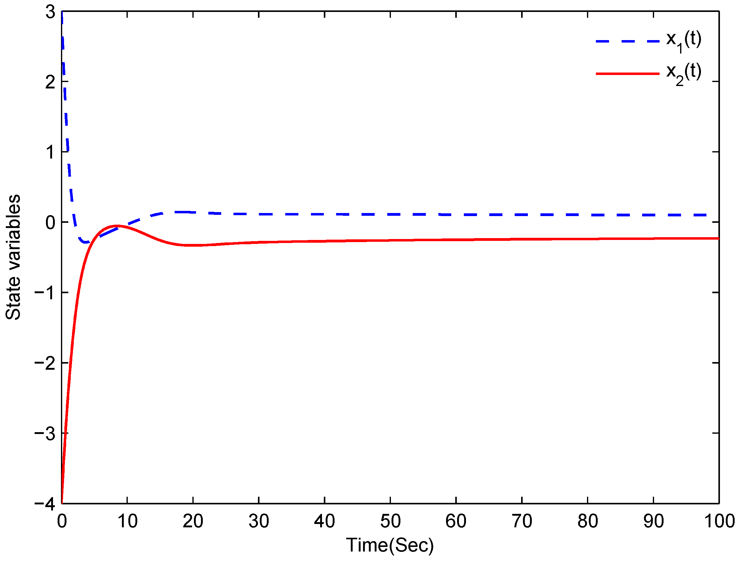
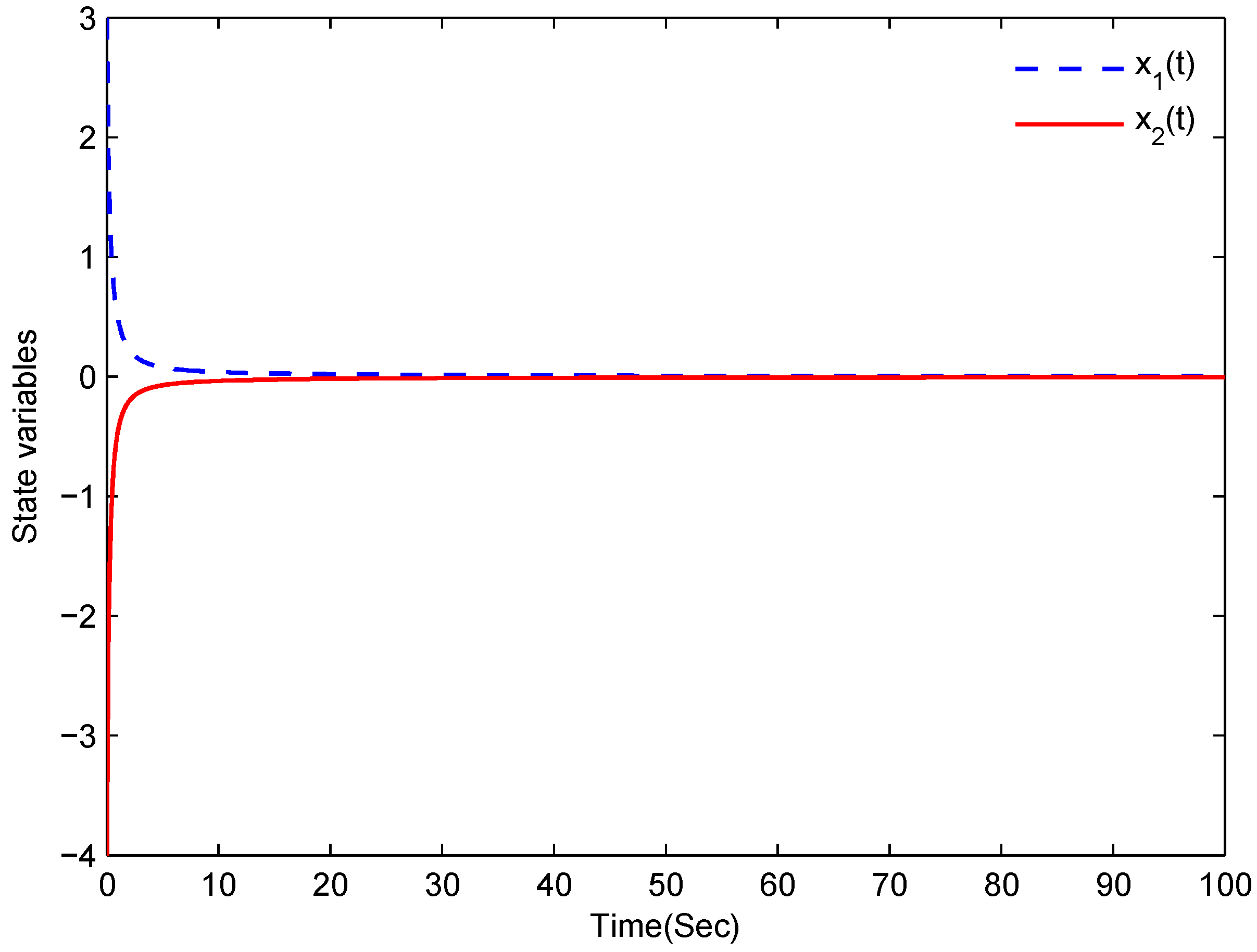
3.2. Stability Analysis

Now, we are ready to establish stability analysis of the FONNs (15).

Theorem 1.

Suppose the following conditions holds:

(1) the nonlinear functions of the FONNs are bounded, i.e.,

$$\left|f_i\left(x_i\left(t\right)\right)\right|\le m_i,$$

(19)

where $m_i>0,i=1,2,\cdots ,n.$

(2) the external bias vector are bounded, i.e., there exist some constants $g_i,i=1,2,\cdots ,n$, such that

$$|I_i|\le g_i.$$

(20)

Then, we have the solution of FONNs (15) will stay bounded, i.e., there exist some positive constants ${\delta }_i$ and $t_1$ such that

$$|x_i\left(t\right)|\le {\delta }_i,$$

(21)

for all i and $t>t_1$.

Proof. 

Taking Laplace transform on (15) yields

$$X_i\left(s\right)=\frac{s^{\alpha -1}}{s^{\alpha }+c_i}{x}_i\left(0\right)+\frac{s^{-1}}{s^{\alpha }+c_i}{I}_i+\frac{1}{s^{\alpha }+c_i}\sum _{j=1}^n{a}_{ij}\mathcal{L}\left(f_j\left(x_j\left(t\right)\right)\right).$$

(22)

According to the property (4), the solution of (15) is given by

$$\begin{array}{cc}\hfill x_i\left(t\right)& =x_i\left(0\right)E_{\alpha ,1}(-c_i{t}^{\alpha })+I_i{t}^{\alpha }{E}_{\alpha ,\alpha +1}(-c_i{t}^{\alpha })\hfill \\ & +\sum _{j=1}^n{a}_{ij}{\int }_0^t{(t-u)}^{\alpha -1}{E}_{\alpha ,\alpha }(-c_i{(t-u)}^{\alpha })f_j\left(x_j\left(u\right)\right)du.\hfill \end{array}$$

(23)

Then, from (19) and (20), we have

$$\begin{array}{cc}\hfill \left|x_i\left(t\right)\right|& \le |x_i\left(0\right)|E_{\alpha ,1}(-c_i{t}^{\alpha })+g_i{t}^{\alpha }{E}_{\alpha ,\alpha +1}(-c_i{t}^{\alpha })\hfill \\ & +\sum _{j=1}^n\left|a_{ij}\right|m_j{\int }_0^t{(t-u)}^{\alpha -1}{E}_{\alpha ,\alpha }(-c_i{(t-u)}^{\alpha })du.\hfill \end{array}$$

(24)

Noting that the Mittag–Leffler function (4) has the following property [36]:

$${\int }_0^t{u}^{\beta -1}{E}_{\alpha ,\beta }(-k{u}^{\alpha })du=t^{\beta }{E}_{\alpha ,\beta +1}(-k{t}^{\alpha }),$$

(25)

we have

$$\left|x_i\left(t\right)\right|\le \left|x_i\left(0\right)\right|E_{\alpha ,1}(-c_i{t}^{\alpha })+(g_i+A_i)t^{\alpha }{E}_{\alpha ,\alpha +1}(-c_i{t}^{\alpha }),$$

(26)

where ${\displaystyle A_i=\sum _{j=1}^n\left|a_{ij}\right|m_j}$.

By using Lemma (3), we have some positive constant $t_0$, for all $t>t_0$, the following inequalities hold:

$$(g_i+A_i)t^{\alpha }{E}_{\alpha ,\alpha +1}(-c_i{t}^{\alpha })\le \frac{g_i+A_i}{c_i}.$$

(27)

According to above discussions, we can conclude that

$$|x_i\left(t\right)|\le {\delta }_i,$$

(28)

where ${\displaystyle {\delta }_i=\underset{1\le i\le n}{max}\left\{\frac{g_i+A_i}{c_i}\right\}}$. This completes the proof. □

Remark 2.

If the system parameters are adjustable, then state variables will tend to an arbitrary small neighborhood of the origin if $c_i$ is large enough.

Remark 3.

The stability analysis for fractional-order linear systems is discussed in [24]. However, in this paper, the model we considered is a nonlinear one which can not be treated as the models in [24]. The results and the analysis methods might be very useful in stability analysis for FONNs.

Remark 4.

In Theorem 1, we give the assumption that $\left|f_i\left(x_i\left(t\right)\right)\right|\le m_i$, where $m_i$ is a positive constant. Actually, the above assumption is not very restricted, since the nonlinear parts in many fractional-order neural networks satisfy this condition. For example, the nonlinear functions in [5,7,10,12,14,16] satisfy $f\left(x\right)=0.5\left(\right|x+\tau |-|x-\tau \left|\right),\tau$ is a constant or $f\left(x\right)=\frac{1}{1+e^x}$.

Theorem 2.

Consider the FONN (16). Suppose that Assumptions 1 and 2 hold. If $\frac{lb}{c}\parallel A\parallel <\alpha$ where ${\displaystyle c=\underset{1\le i\le n}{max}{c}_i}$, then the solution $x\left(t\right)$ of FONN (16) converge to zero.

Proof. 

Suppose that $y\left(t\right)\in R^n$ are two arbitrary solutions of FONN (16). Defining $e\left(t\right)=x\left(t\right)-y\left(t\right)$, as a result, we can obtain

$${}_0^C{D}_t^{\alpha }e\left(t\right)=-Ce\left(t\right)+A(f\left(x\left(t\right)\right)-f\left(y\left(t\right)\right)).$$

(29)

Using the Laplace transform, (29) can be written as

$$s^{\alpha }E\left(s\right)=s^{\alpha -1}e\left(0\right)-CE\left(s\right)+A\mathcal{L}\{f\left(x\left(t\right)\right)-f\left(y\left(t\right)\right)\}.$$

(30)

By some straightforward manipulators, we can obtain

$$E\left(s\right)={(I{s}^{\alpha }+C)}^{-1}(s^{\alpha -1}e\left(0\right)+A\mathcal{L}\{f\left(x\left(t\right)\right)-f\left(y\left(t\right)\right)\}).$$

(31)

Therefore,

$$\begin{array}{cc}e\left(t\right)& =E_{\alpha ,1}(-C{t}^{\alpha })e\left(0\right)+A{\int }_0^t{(t-u)}^{\alpha -1}{E}_{\alpha ,\alpha }(-C{(t-u)}^{\alpha })\mathcal{L}\{f\left(x\left(t\right)\right)-f\left(y\left(t\right)\right)\})du.\end{array}$$

(32)

From Assumption 2 and Lemma 1, we give a constant $b>0$ such that

$$\parallel e\left(t\right)\parallel \le \frac{b\parallel e\left(0\right)\parallel }{1+\parallel C\parallel t^{\alpha }}+lb\parallel A\parallel {\int }_0^t\frac{{(t-u)}^{\alpha -1}}{1+{\parallel C\parallel (t-u)}^{\alpha }}\parallel e\left(u\right)\parallel du.$$

(33)

By applying Lemma 2, we have

$$\begin{array}{cc}\hfill \parallel e\left(t\right)\parallel & \le \frac{b\parallel e\left(0\right)\parallel }{1+\parallel C\parallel t^{\alpha }}\hfill \\ & +{\int }_0^t\frac{{lb\parallel A\parallel (t-u)}^{\alpha -1}\parallel e\left(0\right)\parallel }{{(1+\parallel C\parallel (t-u)}^{\alpha }\left)\right(1+\parallel C\parallel u^{\alpha })}exp\left({\int }_u^t\frac{{lb\parallel A\parallel (t-v)}^{\alpha -1}}{1+{\parallel C\parallel (t-v)}^{\alpha }}dv\right)du\hfill \\ & =\frac{b\parallel e\left(0\right)\parallel }{1+\parallel C\parallel t^{\alpha }}+{\int }_0^t\frac{{bl\parallel A\parallel (t-u)}^{\alpha -1}\parallel e\left(0\right)\parallel }{(1+\parallel C\parallel u^{\alpha }\left)\right(1+{\parallel C\parallel (t-u)}^{\alpha }{)}^{1-\frac{b}{\alpha \parallel C\parallel }}}du\hfill \\ & \le \frac{b\parallel e\left(0\right)\parallel }{1+\parallel C\parallel t^{\alpha }}+{lb\parallel A\parallel \parallel e\left(0\right)\parallel \parallel C\parallel }^{\frac{lb\parallel A\parallel }{\alpha \parallel C\parallel }-2}{\int }_0^t{(t-u)}^{\frac{lb\parallel A\parallel }{\parallel C\parallel }-1}{u}^{-\alpha }du\hfill \\ & =\frac{b\parallel e\left(0\right)\parallel }{1+\parallel C\parallel t^{\alpha }}+{lb\parallel A\parallel |e\left(0\right)\parallel \parallel C\parallel }^{\frac{lb\parallel A\parallel }{\alpha \parallel C\parallel }-2}\frac{\Gamma \left(\frac{lb\parallel A\parallel }{\parallel C\parallel }\right)\Gamma (1-\alpha )}{\Gamma \left(1+\frac{lb\parallel A\parallel }{\parallel C\parallel }-\alpha \right)}{t}^{\frac{lb\parallel A\parallel }{\parallel C\parallel }-\alpha }.\hfill \end{array}$$

(34)

Since $\frac{lb}{c}\parallel A\parallel <\alpha$ where ${\displaystyle c=\parallel C\parallel =\underset{1\le i\le n}{max}{c}_i}$, then (34) leads to

$$\underset{t\to \infty }{lim}\parallel e\left(t\right)\parallel =0,$$

(35)

and this completes the proof. □

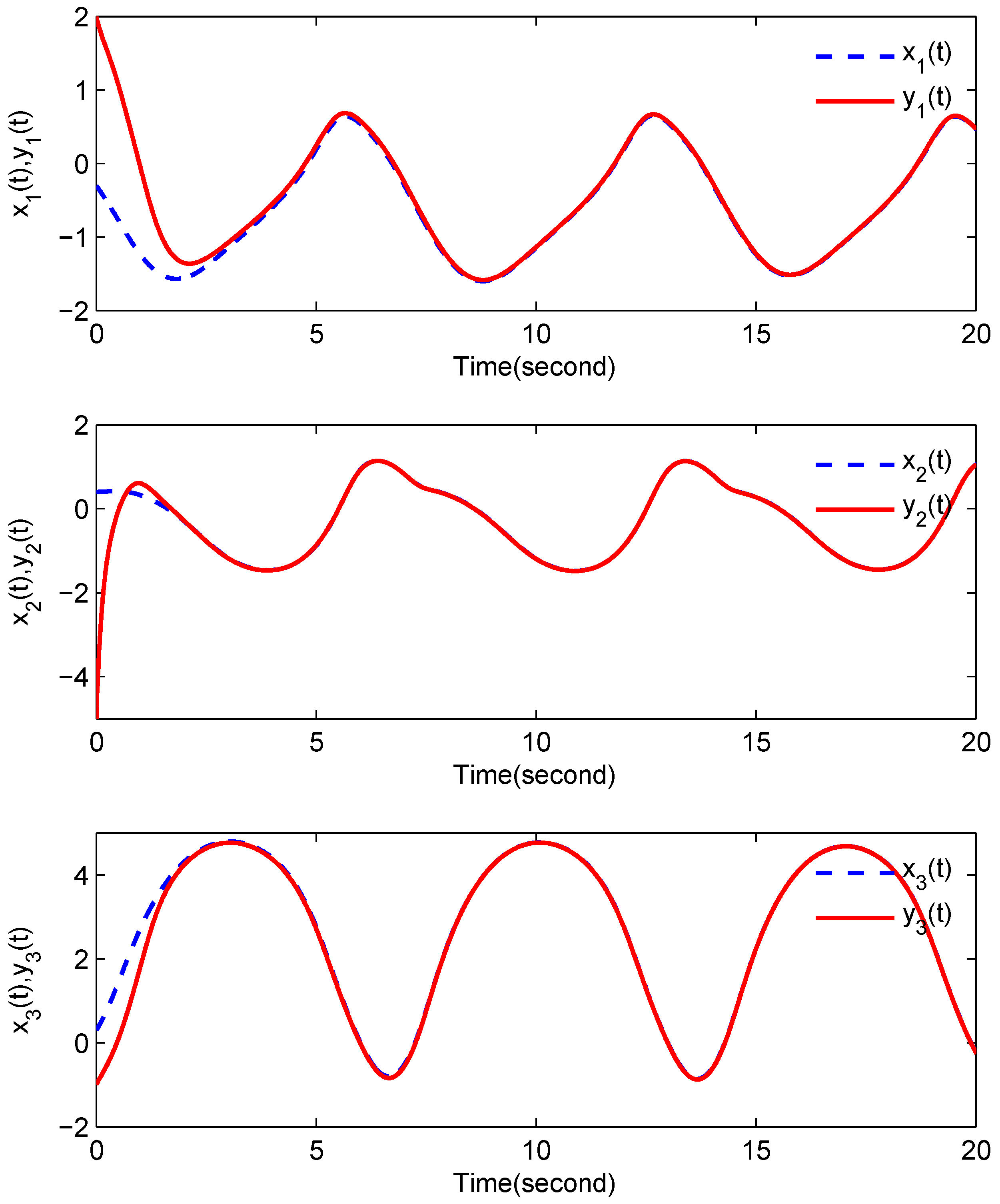
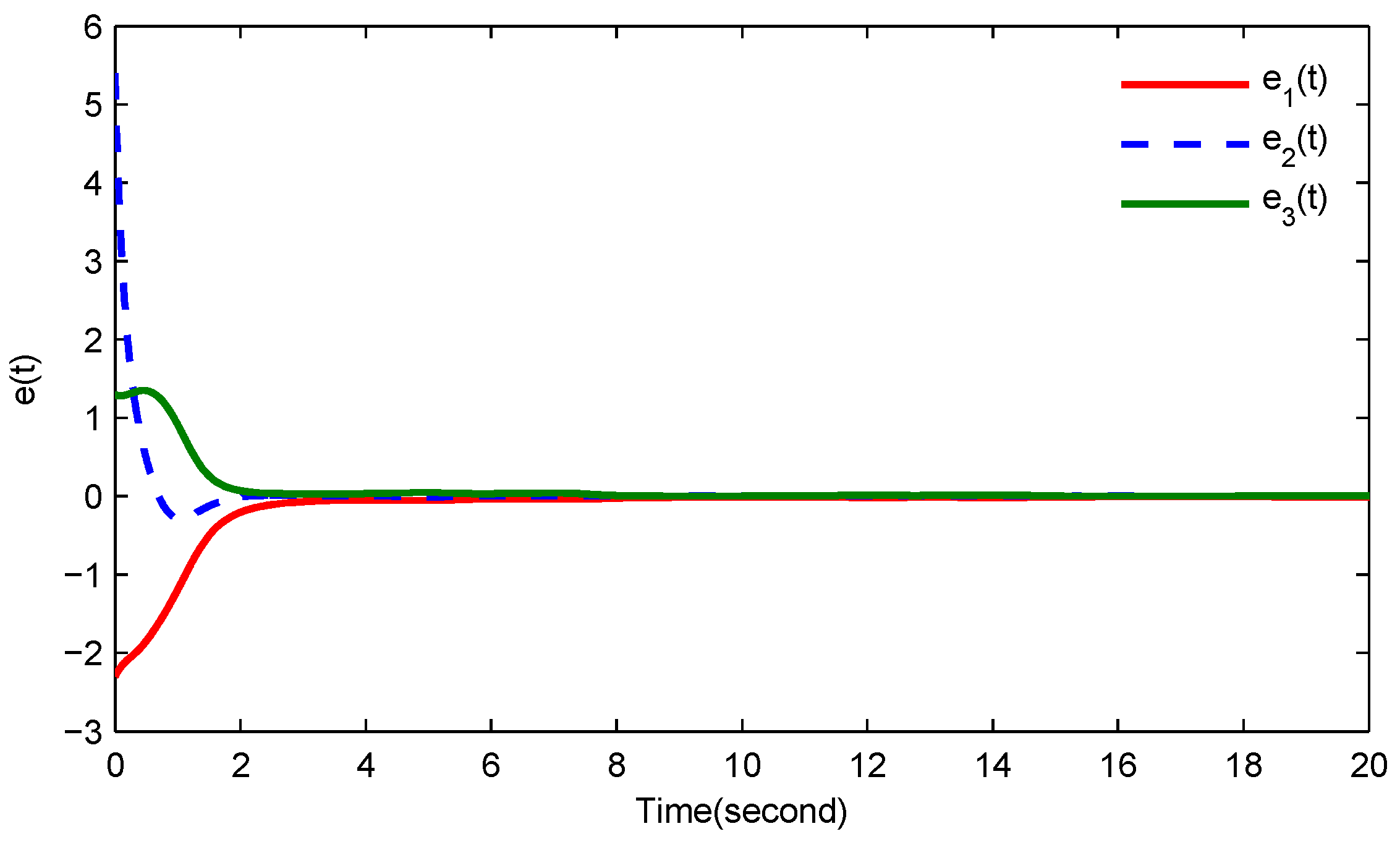
3.3. Synchronization

Let us discuss the synchronization of FONN by utilizing linear control. Let system (16) be the drive system, and the response system be

$${}_0^C{D}_t^{\alpha }{y}_i\left(t\right)=-c_i{y}_i\left(t\right)+\sum _{j=1}^n{a}_{ij}{f}_j\left(y_j\left(t\right)\right)+I_i+{\omega }_i\left(t\right),$$

(36)

or equivalently

$${}_0^C{D}_t^{\alpha }y\left(t\right)=-Cy\left(t\right)+Af\left(y\left(t\right)\right)+I+\omega \left(t\right),$$

(37)

where $\omega \left(t\right)\in R^n$ is a suitable controller which will be given later.

Let $e\left(t\right)=y\left(t\right)-x\left(t\right)$, then

$${}_0^C{D}_t^{\alpha }e\left(t\right)=-Ce\left(t\right)+Ag\left(e\left(t\right)\right)+\omega \left(t\right),$$

(38)

where $g\left(e\right(t\left)\right)=f\left(y\right(t\left)\right)-f\left(x\right(t\left)\right)$.

The controller $\omega \left(t\right)$ can be presented by

$$\omega \left(t\right)=-Ke\left(t\right),$$

where the gain matrix $K=\mathrm{diag}(k_1,\cdots ,k_n)$ with $k_i>0$. The error dynamical system (38) can be described by

$${}_0^C{D}_t^{\alpha }e\left(t\right)=-(C+K)e\left(t\right)+Ag\left(e\left(t\right)\right).$$

(39)

Theorem 3.

If Assumption 2 is satisfied, then systems (16) and (37) are synchronized if the gain matrix K is chosen such that

$$2(C+K)-A{A}^T-L^{T}L>0,$$

(40)

where $L=diag(l_1,l_2\cdots ,l_n)$.

Proof. 

Let the Lyapunov function be

$$V\left(t\right)=e^T\left(t\right)e\left(t\right).$$

According to Lemma 5, we have

$$\begin{array}{cc}\hfill {}_0^C{D}_t^{\alpha }V\left(t\right)& {=}_0^C{D}_t^{\alpha }{e}^T\left(t\right)e\left(t\right)\hfill \\ & \le 2e^T{\left(t\right)}_0^C{D}_t^{\alpha }e\left(t\right)\hfill \\ & =2e^T\left(t\right)[-(C+K)e\left(t\right)+Ag\left(e\left(t\right)\right)]\hfill \\ & =e^T\left(t\right)[-(2C+2K)]e\left(t\right)+2e^T\left(t\right)Ag\left(e\left(t\right)\right).\hfill \end{array}$$

(41)

It follows from Assumption 2 and Lemma 6 that

$$\begin{array}{cc}\hfill 2e^T\left(t\right)Ag\left(e\left(t\right)\right)& \le e^T\left(t\right)A{A}^{T}e\left(t\right)+g{\left(e\left(t\right)\right)}^{T}g\left(e\left(t\right)\right)\hfill \\ & \le e^T\left(t\right)(A{A}^T+L^{T}L)e\left(t\right).\hfill \end{array}$$

(42)

Substituting (42) into Equation (41), we have

$$\begin{array}{cc}\hfill {}_0^C{D}_t^{\alpha }V\left(t\right)& \le -e^T\left(t\right)[2(C+K)-A{A}^T-L^{T}L]e\left(t\right)\hfill \\ & \le -{\lambda }_{min}V\left(t\right),\hfill \end{array}$$

(43)

where ${\lambda }_{min}$ is the minimum eigenvalue of $2(C+K)-A{A}^T-L^{T}L$. Then it follows from Lemma 4 and Lemma 7 that ${lim}_{t\to \infty }\parallel e\left(t\right)\parallel =0$. This ends the proof of Theorem 3. □

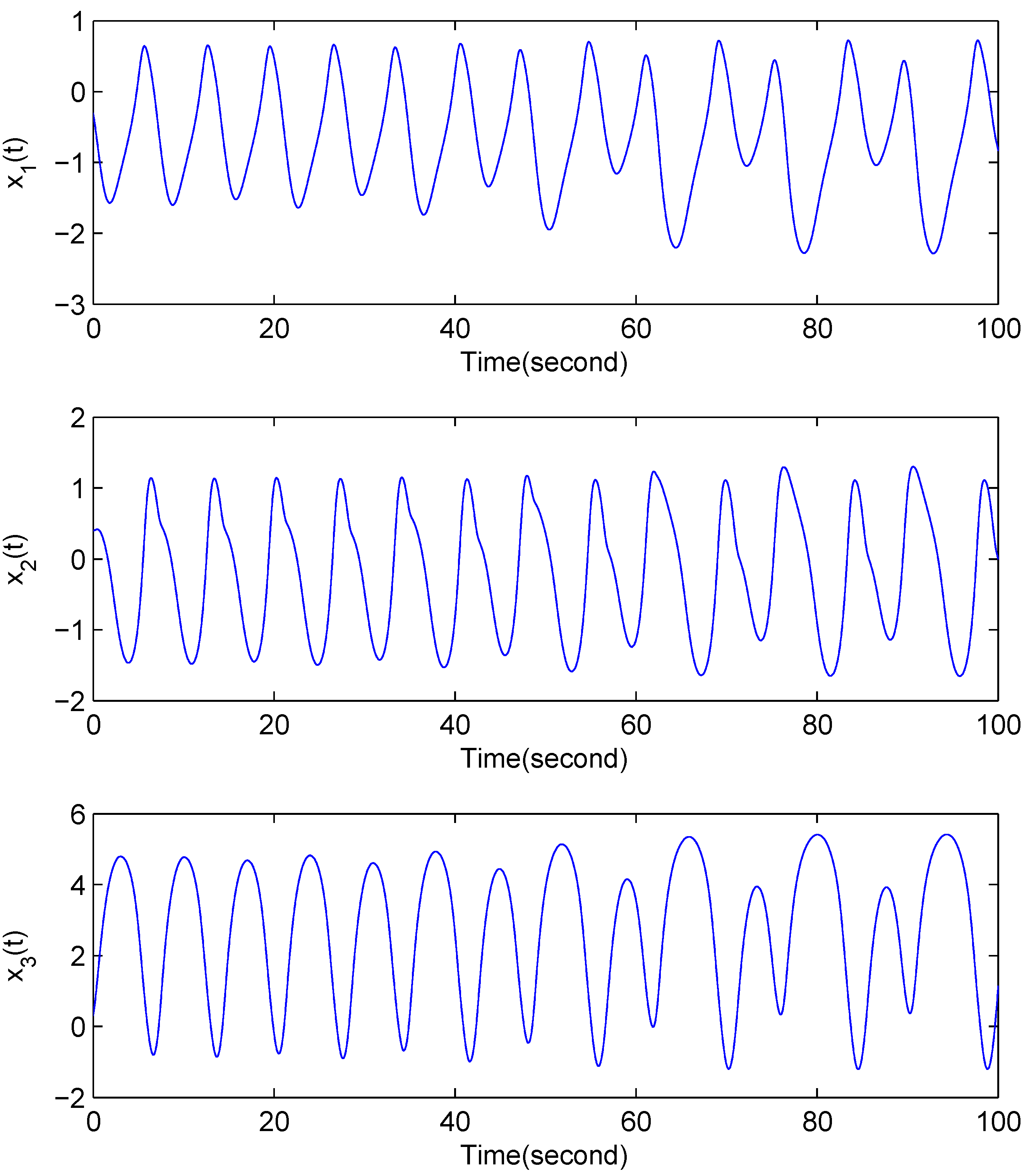
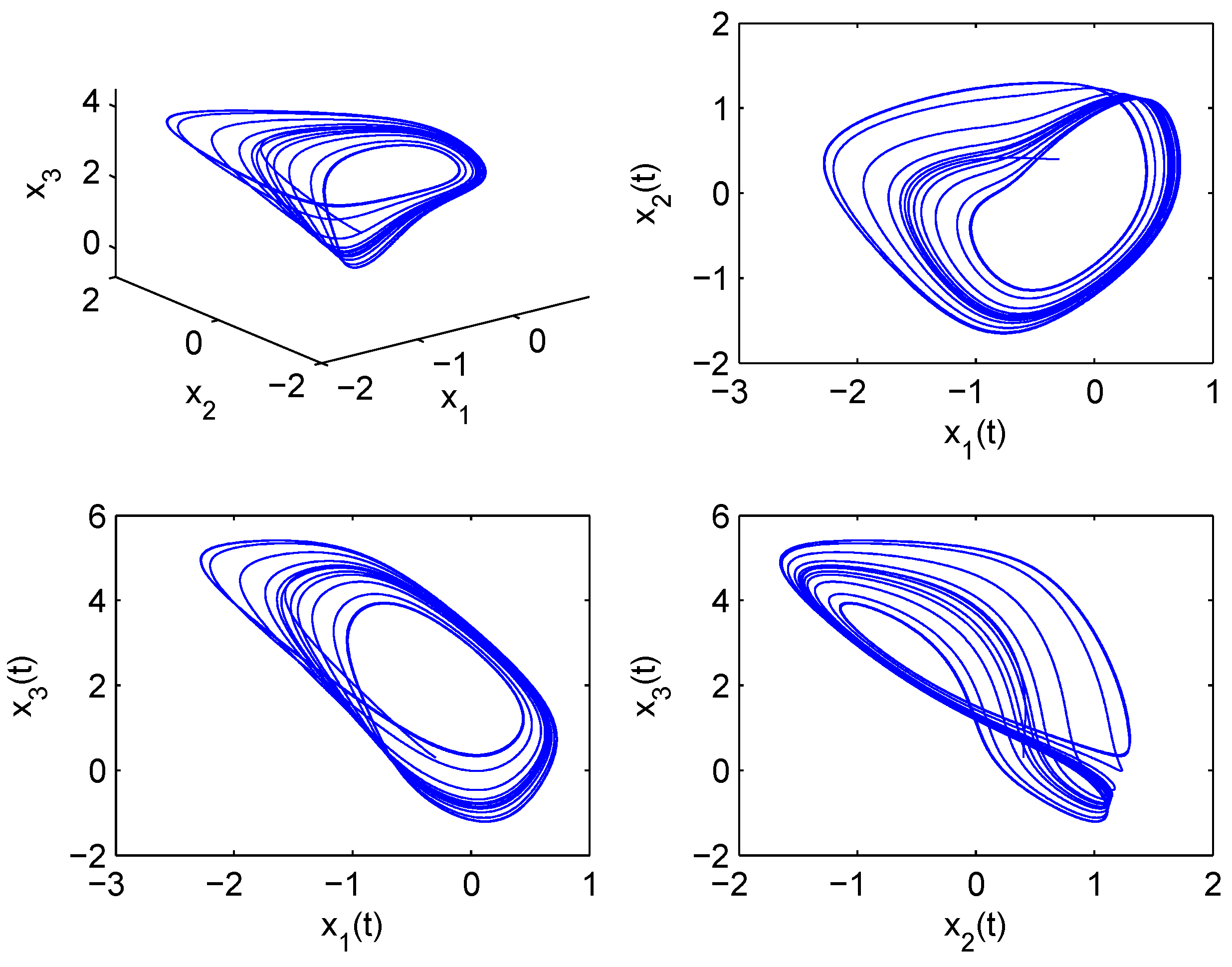
4. Simulation Results

Example 1.

Consider the following two-dimensional FONN:

$$\left\{\begin{array}{cc}\hfill {}_0^C{D}_t^{\alpha }{x}_1=& -c_1{x}_1+0.5arctan{x}_1+cos{x}_2-1,\hfill \\ \hfill {}_0^C{D}_t^{\alpha }{x}_2=& -c_2{x}_1-0.9arctan{x}_1-0.7cos{x}_2+0.7.\hfill \end{array}\right.$$

(44)

Let the initial conditions be $x_1\left(0\right)=3,x_2\left(0\right)=-4$, the fractional order $\alpha =0.88$. Obviously, ${[0,0]}^T$ is a the equilibrium point of (44), which means that Assumption 1 is satisfied.

Firstly, let the system parameters be $c_1=0.3,c_2=0.35$. From the model of FONN (44), we can easily know that the nonlinear functions and the external biases are all bounded, which means the conditions (19) and (20) in Theorem 1 are matched. The time responses of the states are depicted in Figure 1.

Figure 1. Boundedness of the solution $x\left(t\right)$ for fractional-order neural network (44) with $c_1=0.3$ and $c_2=0.35$.

Figure 1. Boundedness of the solution $x\left(t\right)$ for fractional-order neural network (44) with $c_1=0.3$ and $c_2=0.35$.

Figure 2. Convergence of the solution $x\left(t\right)$ for fractional-order neural network (44) with $c_1=2$ and $c_2=3$.

Figure 2. Convergence of the solution $x\left(t\right)$ for fractional-order neural network (44) with $c_1=2$ and $c_2=3$.

Then, let $c_1=2$, $c_2=3$ and $b=1$. From the model of FONN (44), we know $\parallel A\parallel =1.2354$ and the nonlinear functions $arctan(·)$ and $cos(·)$ satisfy the Lipshitz condition. The Lipshitz constant l can be chosen as $l=1$, which means that Assumption 2 is satisfied. From the above discussions, we have $\frac{lb\parallel A\parallel }{c}=\frac{1.2354}{3}=0.4118<\alpha$. Then, from Theorem 2, we know the solution of FONNs (44) converge to zero asymptotically. The simulation results are presented in Figure 2.

Example 2.

In system (16), let $\alpha =0.95,$ $x\left(t\right)={(x_1\left(t\right),x_2\left(t\right),x_3\left(t\right))}^T,$ $C=\mathrm{diag}(1,1,1),$ $I_1=I_2=I_3=0,$ $f\left(x\left(t\right)\right)={(tanh\left(x_1\left(t\right)\right),tanh\left(x_2\left(t\right)\right),tanh\left(x_3\left(t\right)\right))}^T,$ and $A=\left[\begin{array}{ccc}2.00& -1.20& 0\\ 1.80& 1.71& 1.15\\ -4.75& 0& 1.10\end{array}\right]$. System (16) satisfies Assumption 2 with $L=\mathrm{diag}(1,1,1)$. Under these parameters, the simulation of chaotic attractor and time responses of state $x\left(t\right)$ for system (16) are shown in Figure 3 and Figure 4.

Figure 3. Time responses of $x\left(t\right)$ of system (16) with initial value ${[-0.3,0.4,0.3]}^T.$

Figure 3. Time responses of $x\left(t\right)$ of system (16) with initial value ${[-0.3,0.4,0.3]}^T.$

Figure 4. Chaotic trajectories of system (16) with initial value ${[-0.3,0.4,0.3]}^T.$

Figure 4. Chaotic trajectories of system (16) with initial value ${[-0.3,0.4,0.3]}^T.$

Figure 5. Synchronization trajectories of (16) and (37).

Figure 5. Synchronization trajectories of (16) and (37).

In response system (37), we chose $k_1=14.4,k_2=13.9,k_3=14.8$. By computation, we know condition (40) is satisfied. Then, it follows from Theorem 3 that synchronization between (16) and (37) will be achieved. Figure 5 and Figure 6 depict the simulation results.

Figure 6. Synchronization errors.

Figure 6. Synchronization errors.

5. Conclusions

The dynamical properties of FONNs are investigated in this paper. First, two sufficient conditions are established for boundedness and convergence of the solution for FONN. Furthermore, based on the Mittag–Leffler function and linear feedback control technique, the synchronization criterion of chaotic FONN is obtained. Compared with the related literature, the conditions we need are easy to satisfy. The effectiveness of the proposed results is further confirmed by numerical simulations.

References

1. Cao, J.; Liang, J. Boundedness and stability for Cohen–Grossberg neural network with time-varying delays. J. Math. Anal. Appl. 2004, 296, 665–685. [Google Scholar] [CrossRef]
2. Cao, J.; Wang, J. Global asymptotic and robust stability of recurrent neural networks with time delays. IEEE Trans. Circuits Syst. I Regul. Pap. 2005, 52, 417–426. [Google Scholar]
3. Zhang, H.; Wang, Z.; Liu, D. Global asymptotic stability and robust stability of a class of Cohen–Grossberg neural networks with mixed delays. IEEE Trans. Circuits Syst. I Regul. Pap. 2009, 56, 616–629. [Google Scholar] [CrossRef]
4. Song, C.; Cao, J. Dynamics in fractional-order neural networks. Neurocomputing 2014, 142, 494–498. [Google Scholar] [CrossRef]
5. Wang, H.; Yu, Y.; Wen, G. Stability analysis of fractional-order hopfield neural networks with time delays. Neural Netw. 2014, 55, 98–109. [Google Scholar] [CrossRef] [PubMed]
6. Lazarević, M. Stability and stabilization of fractional order time delay systems. Sci. Tech. Rev. 2011, 61, 31–45. [Google Scholar]
7. Liu, H.; Li, S.; Wang, H.; Huo, Y.; Luo, J. Adaptive synchronization for a class of uncertain fractional-order neural networks. Entropy 2015, 17, 7185–7200. [Google Scholar] [CrossRef]
8. Anastassiou, G.A. Fractional neural network approximation. Comput. Math. Appl. 2012, 64, 1655–1676. [Google Scholar] [CrossRef]
9. Liu, H.; Li, S.; Sun, Y.; Wang, H. Prescribed performance synchronization for fractional-order chaotic systems. Chin. Phys. B 2015, 24, 153–160. [Google Scholar] [CrossRef]
10. Chen, L.; Chai, Y.; Wu, R.; Ma, T.; Zhai, H. Dynamic analysis of a class of fractional-order neural networks with delay. Neurocomputing 2013, 111, 190–194. [Google Scholar] [CrossRef]
11. Liu, H.; Li, S.; Sun, Y.; Wang, H. Adaptive fuzzy synchronization for uncertain fractional-order chaotic systems with unknown non-symmetrical control gain. Acta Phys. Sinaca 2015, 64, 70503. [Google Scholar]
12. Kaslik, E.; Sivasundaram, S. Nonlinear dynamics and chaos in fractional-order neural networks. Neural Netw. 2012, 32, 245–256. [Google Scholar] [CrossRef] [PubMed]
13. Arena, P.; Caponetto, R.; Fortuna, L.; Porto, D. Bifurcation and chaos in noninteger order cellular neural networks. Int. J. Bifurc. Chaos 1998, 8, 1527–1539. [Google Scholar] [CrossRef]
14. Huang, X.; Zhao, Z.; Wang, Z.; Li, Y. Chaos and hyperchaos in fractional-order cellular neural networks. Neurocomputing 2012, 94, 13–21. [Google Scholar] [CrossRef]
15. Boroomand, A.; Menhaj, M.B. Fractional-order hopfield neural networks. In Advances in Neuro-Information Processing; Springer-Verlag: Berlin/Heidelberg, Germany, 2009. [Google Scholar]
16. Chen, J.; Zeng, Z.; Jiang, P. Global Mittag-Leffler stability and synchronization of memristor-based fractional-order neural networks. Neural Netw. 2014, 51, 1–8. [Google Scholar] [CrossRef] [PubMed]
17. Wen, G.; Hu, G.; Yu, W.; Cao, J.; Chen, G. Consensus tracking for higher-order multi-agent systems with switching directed topologies and occasionally missing control inputs. Sys. Control Lett. 2013, 62, 1151–1158. [Google Scholar] [CrossRef]
18. Wen, G.; Hu, G.; Yu, W.; Chen, G. Distributed consensus of higher order multiagent systems with switching topologies. IEEE Trans. Circuits Syst. II Express Br. 2014, 61, 359–363. [Google Scholar]
19. Chen, L.; Chai, Y.; Wu, R.; Yang, J. Stability and stabilization of a class of nonlinear fractional-order systems with caputo derivative. IEEE Trans. Circuits Syst. II Express Br. 2012, 59, 602–606. [Google Scholar] [CrossRef]
20. Ahn, H.S.; Chen, Y. Necessary and sufficient stability condition of fractional-order interval linear systems. Automatica 2008, 44, 2985–2988. [Google Scholar] [CrossRef]
21. Shen, J.; Lam, J. Non-existence of finite-time stable equilibria in fractional-order nonlinear systems. Automatica 2014, 50, 547–551. [Google Scholar] [CrossRef]
22. Zheng, C.; Li, N.; Cao, J. Matrix measure based stability criteria for high-order neural networks with proportional delay. Neurocomputing 2015, 149, 1149–1154. [Google Scholar] [CrossRef]
23. Nie, X.; Zheng, W.; Cao, J. Multistability of memristive Cohen–Grossberg neural networks with non-monotonic piecewise linear activation functions and time-varying delays. Neural Netw. 2015, 71, 27–36. [Google Scholar] [CrossRef] [PubMed]
24. Matignon, D. Stability results for fractional differential equations with applications to control processing. Comput. Eng. Syst. Appl. 1996, 2, 963–968. [Google Scholar]
25. Farges, C.; Moze, M.; Sabatier, J. Pseudo-state feedback stabilization of commensurate fractional order systems. Automatica 2010, 46, 1730–1734. [Google Scholar] [CrossRef]
26. Ren, F.; Cao, F.; Cao, J. Mittag–Leffler stability and generalized Mittag–Leffler stability of fractional-order gene regulatory networks. Neurocompu. 2015, 160, 185–190. [Google Scholar] [CrossRef]
27. Rakkiyappan, R.; Velmurugan, G.; Cao, J. Stability analysis of fractional-order complex-valued neural networks with time delays. Chaos Solitons Fractals 2015, 78, 297–316. [Google Scholar] [CrossRef]
28. Trigeassou, J.C.; Maamri, N.; Sabatier, J.; Oustaloup, A. A lyapunov approach to the stability of fractional differential equations. Signal Process. 2011, 91, 437–445. [Google Scholar] [CrossRef]
29. Yu, J.; Hu, C.; Jiang, H. α-stability and α-synchronization for fractional-order neural networks. Neural Netw. 2012, 35, 82–87. [Google Scholar] [CrossRef] [PubMed]
30. Li, K.; Peng, J.; Gao, J. A comment on α-stability and α-synchronization for fractional-order neural networks. Neural Netw. 2013, 48, 207–208. [Google Scholar]
31. Wang, K.; Teng, Z.; Jiang, H. Adaptive synchronization in an array of linearly coupled neural networks with reaction–diffusion terms and time delays. Commun. Nonlinear Sci. Numer. Simul. 2012, 17, 3866–3875. [Google Scholar] [CrossRef]
32. Zhang, D.; Xu, J. Projective synchronization of different chaotic time-delayed neural networks based on integral sliding mode controller. Appl. Math. Comput. 2010, 217, 164–174. [Google Scholar] [CrossRef]
33. Yang, X.; Cao, J. Stochastic synchronization of coupled neural networks with intermittent control. Phys. Lett. A 2009, 373, 3259–3272. [Google Scholar] [CrossRef]
34. Zhang, G.; Shen, Y.; Wang, L. Global anti-synchronization of a class of chaotic memristive neural networks with time-varying delays. Neural netw. 2013, 46, 1–8. [Google Scholar] [CrossRef] [PubMed]
35. Lu, J.; Ho, D.; Cao, J. A unified synchronization criterion for impulsive dynamical networks. Automatica 2010, 4, 1215–1221. [Google Scholar] [CrossRef]
36. Podlubny, I. Fractional differential equations. Soc. Ind. Appl. Math. 2000, 42, 766–768. [Google Scholar]
37. Luo, J.; Li, G.; Liu, H. Linear control of fractional-order financial chaotic systems with input saturation. Discret. Dyn. Nature Soc. 2014. [Google Scholar] [CrossRef]
38. Li, Y.; Chen, Y.; Podlubny, I. Mittag–Leffler stability of fractional order nonlinear dynamic systems. Automatica 2009, 45, 1965–1969. [Google Scholar] [CrossRef]
39. Aguila-Camacho, N.; Duarte-Mermoud, M.A.; Gallegos, J.A. Lyapunov functions for fractional order systems. Commun. Nonlinear Sci. Numer. Simul. 2014, 19, 2951–2957. [Google Scholar] [CrossRef]