Fractal Representation of Exergy ^†

Abstract

We developed a geometrical model to represent the thermodynamic concepts of exergy and anergy. The model leads to multi-scale energy lines (correlons) that we characterised by fractal dimension and entropy analyses. A specific attention will be paid to overlapping points, rising interesting remarks about trans-scale dynamics of heat flows.

1. Introduction

During the last decades, the formalism of thermodynamics has been applied to chaotic phenomena, fractal, multifractal and many other complex systems. A thermodynamics of chaotic systems, fractal signals and fractal networks has emerged; its history is detailed in the book of Beck and Schlögl [1]. These intensive works on the concept of scale associated to a miniaturization of components in electronics, have led to a new way of thinking. The general hypothesis of continuity is invalid and heat transfer at micro- and nano-scales exhibits fractal features (e.g., [2,3]). These studies have readdressed the difficulty of interpreting the notion of temperature, which sometimes needs a new definition depending on the physical system under consideration. More generally, a geometry of thermodynamics is needed. This is the goal of recent theories such as the constructal theory [4,5,6] which first formalised the question of scale optimisation. In this framework, an elementary optimized configuration is reproduced at every scale, from small to large, to maximize the overall efficiency. Another approach to this question is made by the entropic-skins theory [7,8,9], which provides a new geometrical framework for the study of scale-dependent fractal systems in terms of diffusion of scale-entropy in scale-space.

Complex systems, and especially heat, are fundamentally fractal in their scale structure and we believe that new tools and models must emerge to support the reflection and look further into this “space into space”. This paper aims to provide a tool to investigate the fractal nature of heat. To do so, we propose to “draw” a heat flow as a multi-scale line reflecting its internal scale complexity, or in other words, its intrinsic quality. This concept of quality is now commonly related to exergy, also called available energy in the early literature. Indeed, it is defined as the maximum extractable work from a given system when bringing it to equilibrium with its surrounding environment by means of ideal processes (of heat, work and eventually mass exchanges). In exergetics, considering a certain amount of fluid receiving some heat $\delta Q$ from its environment and providing some work $\delta W$ to it, the change in its internal exergy $d\xi$ is given by Gouy-Stodola equation [6]:

$$d\xi =\left(1-\frac{T_0}{T}\right)\delta Q+\delta W-T_0\Pi$$

(1)

where T and $T_0$ are the temperatures (expressed in Kelvin) of the fluid and its environment respectively, and Π is the total entropy generation. The first term on the right-hand side of Equation (1) is called heat exergy $dX=\theta \delta Q$, where we have introduced the Carnot factor:

$$\theta =1-\frac{T_0}{T}$$

(2)

In this paper, we restrict our attention to heat exergy but we believe that the toy model presented in the followings may be adapted to other forms of exergy. The supplement of exergy is called anergy, it is the part of heat that cannot be extracted and is expressed as follows:

$$dA=\left(1-\theta \right)\delta Q=\frac{T_0}{T}\delta Q=T_{0}dS$$

(3)

where we used Clausius definition of entropy in the last equality. These two antagonist components of energy are, however, related. To picture it, let us consider a turbine activated by a heated gas. The exergetic part of the fluid may be seen as the one directly hurting the rotor blades, while the anergetic one helps the former to reach the blades through interactions but ultimately misses them (i.e., the velocity vector of the corresponding particles is not properly oriented). From this point of view, anergy may be seen as a conductor, or more precisely, a support for exergy.

The Carnot factor (Equation (2)) holds in the case of heat transferred on macro-continua (e.g., solids, fluids) according to Fourier’s law. In the case of thermal radiations, in the cosmic background medium for instance, the energy flux density I scales as $T^4$ according to Stefan–Boltzmann law. The expression for the ratio ${\theta }^{*}=J/I$, where J is the corresponding exergy flux density, may then depend on the emissivity of the emitting body and the wave frequency of the beam, see [10,11] for detailed analyses on the subject. For simplicity, in the followings, we restrict our discussion to the case of heat transferred on macro-continua, but the results and interpretations will hold as long as θ (or equivalently ${\theta }^{*}$) will be concerned. The conclusions in terms of temperature will need more careful attention.

Despite clarifying discussions (e.g., [12,13]), entropy, and moreover the distinction between exergy and anergy, may be puzzling. We believe that the geometrical representation proposed in this paper will provide insights to the question of the nature of heat as a trans-scale phenomenon.

2. Description of the Toy Model

This toy model has been motivated by the idea that a pure exergetic flow (of work or heat at $T\to \infty$) may be pictured as a straight line (as for laminar flows or directed bursts) while a degraded heat flow (finite temperature) would exhibit more structural features (as for turbulent flows). In order to draw a conceptual link from microscopic behaviour to large scale observables, we build the trajectory of a heat quantum (in the sense of a small quantity of heat) placed on a plane lattice and acting on a hypothetical piston by means of probabilistic evolution rules. The resulting large scale path is called a correlon in the following.

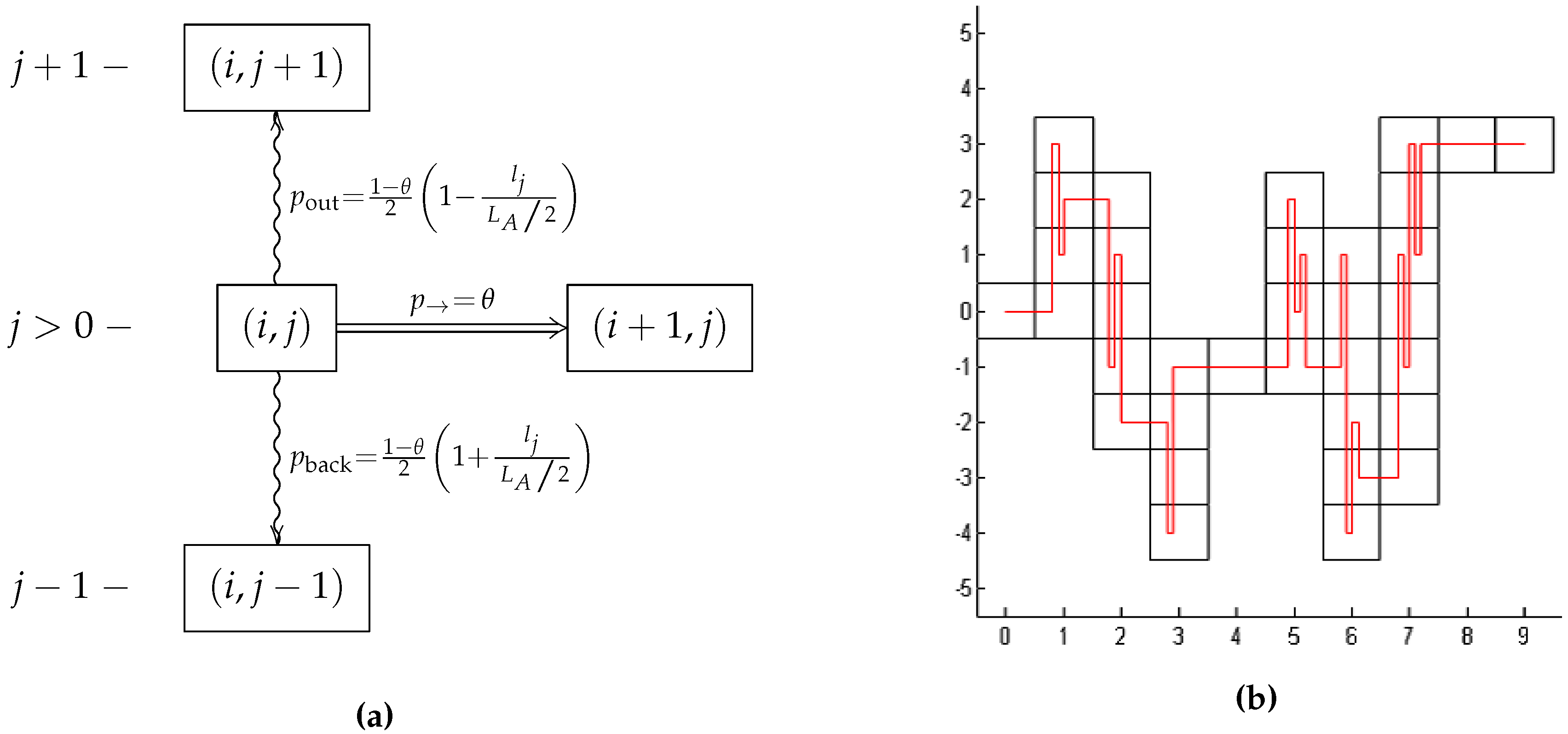
To build up the correlon corresponding to a given heat load, we assimilate the energy content Q to the total movement capacity of the heat quantum. We make this analogy in defining $N_Q\sim Q$, the total number of elementary steps at disposal to push the hypothetical piston. The quantum is originally placed on the left side of a plane, at coordinate $(i=0,j=0)$, right behind the hypothetical piston. Step by step, the quantum may push the piston by one increment to the right $(i,j)\to (i+1,j)$, or diffuse on the side $(i,j)\to (i,j\pm 1)$, see Figure 1. In doing so, the quantum gives out the quantity $q=Q/N_Q$ to every crossed lattice point to heat it up and will stop after the allowed $N_Q$ steps. The distance between two lattice points $l_c$ have been arbitrarily set to 1. From a different point of view, one can consider a heat source providing quanta of value $q=Q/N_Q$ one after another, to heat up the plane. In this picture, each heat quantum creates a displacement equal to $l_c$, the minimal distance (i.e., between two lattice points). When the quantum is pure exergetic, the displacement is longitudinal (i.e., going to the right if the heat source is on the left side on the plane). Conversely, if the quantum is pure anergetic, the displacement is lateral.

Figure 1. Algorithm for the building of a correlon (a) and diagram of a typical trajectory (b). (a) Probabilities of diffusion of the heat quantum for j > 0 (p_out and p_back are inverted otherwise); (b) Diagram of a correlon obtain for θ = 0.15 and N_Q = 60.

Figure 1. Algorithm for the building of a correlon (a) and diagram of a typical trajectory (b). (a) Probabilities of diffusion of the heat quantum for j > 0 (p_out and p_back are inverted otherwise); (b) Diagram of a correlon obtain for θ = 0.15 and N_Q = 60.

Since exergy is the available part of energy, the Carnot factor (Equation (2)) is taken to define the probability $p_{\to }$ to push the piston further to the right:

$$p_{\to }=\theta$$

(4)

While the forward movement is driven by the exergy fraction of heat, the side diffusion is assumed constrained by its anergy part. This comes down to consider anergy as a “structural strength” that pulls back the diffusing heat quantum to the central line ($j=0$). This “exergy canal” may thus be seen as plunged in an anergetic duct of size $L_A=(1-\theta )N_Q{l}_c$, which restrains the side diffusion. The induced restoring force is considered spring like: further is the quantum from the central line, stronger is the restoring force. Hence, the pull-back probability is defined as follows:

$$p_{\mathrm{back}}=\frac{1-\theta }{2}\left(1+\frac{l_j}{L_A/2}\right)$$

(5)

where $l_j=\left|j\right|l_c$ is the distance of the quantum from the central line. These probabilities are summarized in Figure 1a and a schematic example of a resulting correlon is given in Figure 1b for $\theta =0.15$ and $N_Q=60$. The red line traces the path followed by the quantum and the black squares indicate the lattice regions successively covered.

3. Correlon Characteristics

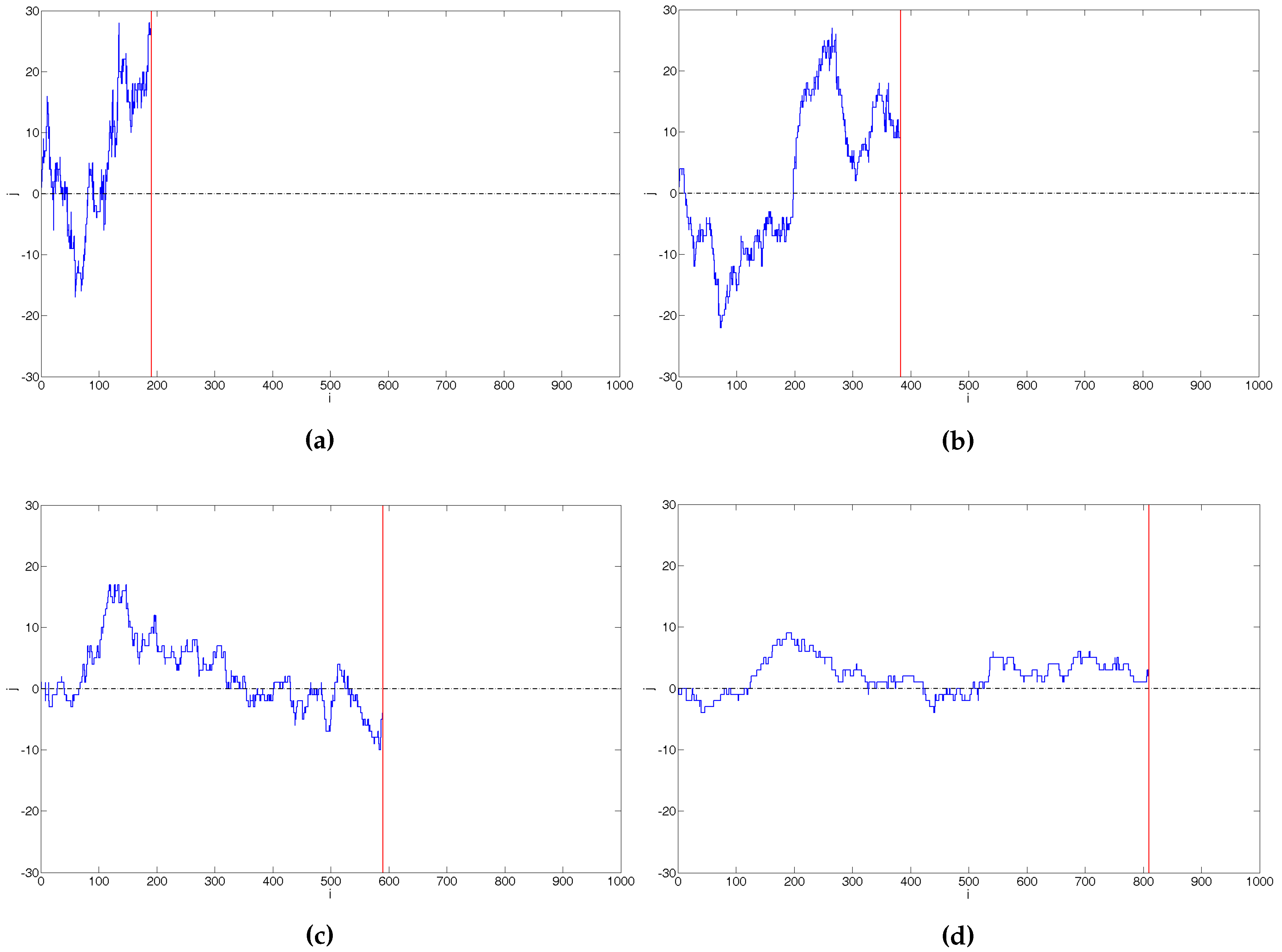
The probabilistic algorithm of Figure 1a has been implemented in Matlab and four examples are shown in Figure 2 for a given heat load at various temperatures. First of all, concerning the global aspect, as expected (due to probability definitions) we see that the resulting length of the correlons (i.e., the distance by which the piston has been pushed) is given by $L_X=N_X{l}_c\simeq \theta N_Q{l}_c$, the analogue for exergy in the model, where $N_X$ is the number of step the quantum has made to the right. Also, the higher the temperature, the lower the side diffusion, i.e., the straighter the line. Table 1 gathers the characteristic quantities of the correlons shown on Figure 2 and their corresponding analogous energetic values. The exergetic (horizontal) lengths are not exactly equal to the corresponding $\theta N_Q{l}_c$ because of the probabilistic behaviour of the heat quantum. However, when averaging over several correlons we find the average $\langle L_X\rangle =\theta N_Q{l}_c$.

Figure 2. Correlons obtained for a given heat load N_Q at four different temperatures. The central line (j = 0) and the hypothetical piston are represented by a black dashed line and a red one respectively. (a) Correlon for θ = 0.2 and N_Q = 1000, N_X = 189, L_A/l_c = 800; (b) Correlon for θ = 0.4 and N_Q = 1000, N_X = 377, L_A/l_c = 600; (c) Correlon for θ = 0.6 and N_Q = 1000, N_X = 583, L_A/l_c = 400; (d) Correlon for θ = 0.8 and N_Q = 1000, N_X = 813, L_A/l_c = 200.

Figure 2. Correlons obtained for a given heat load N_Q at four different temperatures. The central line (j = 0) and the hypothetical piston are represented by a black dashed line and a red one respectively. (a) Correlon for θ = 0.2 and N_Q = 1000, N_X = 189, L_A/l_c = 800; (b) Correlon for θ = 0.4 and N_Q = 1000, N_X = 377, L_A/l_c = 600; (c) Correlon for θ = 0.6 and N_Q = 1000, N_X = 583, L_A/l_c = 400; (d) Correlon for θ = 0.8 and N_Q = 1000, N_X = 813, L_A/l_c = 200.

Table 1. Characteristic quantities of the correlons shown on Figure 2 and their corresponding analogous energetic values.

Figure	θ	Num. of Quantum Movement (NQ)	Energy (Q)	Horizontal Length (LX)	Exergy (X)	Duct Length (LA)	Anergy (A)
2a	0.2	1000	$1000q$	$189l_c$	$200q$	$800l_c$	$800q$
2b	0.4	1000	$1000q$	$377l_c$	$400q$	$600l_c$	$600q$
2c	0.6	1000	$1000q$	$583l_c$	$600q$	$400l_c$	$400q$
2d	0.8	1000	$1000q$	$813l_c$	$800q$	$200l_c$	$200q$

Table 1. Characteristic quantities of the correlons shown on Figure 2 and their corresponding analogous energetic values.

Figure	θ	Num. of Quantum Movement (NQ)	Energy (Q)	Horizontal Length (LX)	Exergy (X)	Duct Length (LA)	Anergy (A)
2a	0.2	1000	$1000q$	$189l_c$	$200q$	$800l_c$	$800q$
2b	0.4	1000	$1000q$	$377l_c$	$400q$	$600l_c$	$600q$
2c	0.6	1000	$1000q$	$583l_c$	$600q$	$400l_c$	$400q$
2d	0.8	1000	$1000q$	$813l_c$	$800q$	$200l_c$	$200q$

Secondly, the trajectories clearly exhibit a fractal behaviour since they present irregularities at every scale; from the integral length $l_0=L_X$ down to the cut-off length $l_c$. Therefore, we measured its fractal properties by using two methods: the box-counting method and the Richardson’s method of the ruler. Our fractal algorithms have been tested successfully on deterministic fractals. We determined both these fractal dimensions in the scale range $[l_c,l_0]$. The box-counting method is fairly straightforward to apply on a plane lattice and the fractal dimension ${\Delta }_{\mathrm{sh}}$ is computed according to the relation: $N\left(l\right)\sim l^{-{\Delta }_{\mathrm{sh}}}$, where N is the number of box of size l needed to cover the correlon. The Richardson method of the ruler consists in measuring the extended length (i.e., with all its foldings) of the correlon, the fractal dimension ${\Delta }_{\mathrm{int}}$ is then given by the relation: $L\left(l\right)\sim l^{1-{\Delta }_{\mathrm{int}}}$. The distinction between ${\Delta }_{\mathrm{sh}}$ and ${\Delta }_{\mathrm{int}}$ will be discussed in the next section. In a second time, in Section 3.2, we investigate the question of entropy for the correlons. In Statistical Physics, the entropy of complex systems is given by Gibbs–Shannon definition:

$$S_G=-k_B\sum _j{p}_{j}ln{p}_j$$

(6)

where $k_B$ is the Boltzmann constant and $p_j$ is the probability of existence of the microstate j. Based on Equation (6), we introduce a definition of entropy for the correlons where $p_j$ is the probability to find the quantum at a distance j from the central line. Treating the overlapping distinctly or not will rise interesting remarks consistent with the discussion about fractal dimension.

3.1. Fractal Behaviour

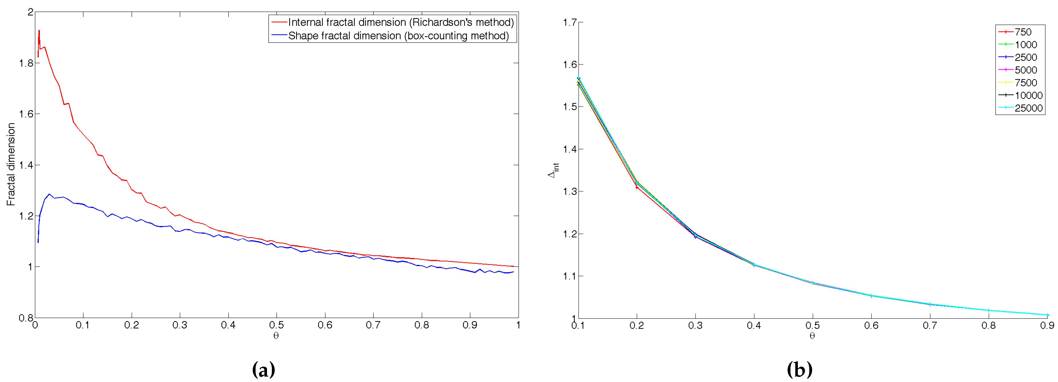
We first use the box-counting method to determine the fractal dimension of the space covered by a given correlon. As mentioned previously, this technique is not sensible to the quantum overlapping movements. Thus, it provides a dimension for the fractal external shape of the correlon, ignoring its internal structure. Therefore, the dimension obtained in this way will be called the correlon shape dimension ${\Delta }_{\mathrm{sh}}$, in blue as a function of θ on Figure 3a. Second, to grasp the internal fractal features (in red on Figure 1b) of the correlon, we use Richardson’s method of the ruler. The dimension hence obtained will be called the correlon internal dimension ${\Delta }_{\mathrm{int}}$, in red as a function of θ on Figure 3a.

Figure 3. Fractal dimensions as functions of θ. The curves are obtained by averaging over 50 correlons for each temperature. (a) Internal and shape fractal dimensions of correlons as functions of θ. (b) Internal fractal dimension ${\Delta }_{\mathrm{int}}$ as a function of θ for various heat loads N_Q in the scale range ${[l_c,l_0]}_{750}$.

Figure 3. Fractal dimensions as functions of θ. The curves are obtained by averaging over 50 correlons for each temperature. (a) Internal and shape fractal dimensions of correlons as functions of θ. (b) Internal fractal dimension ${\Delta }_{\mathrm{int}}$ as a function of θ for various heat loads N_Q in the scale range ${[l_c,l_0]}_{750}$.

First, the correlon internal dimension obtained with Richardson’s method. It tends to the embedding space dimension $d=2$ as $\theta \to 0$ and to the topological one $d=1$ when $\theta \to 1$. At large temperature, this is not surprising since we built our model on the idea that a high exergetic flow of heat is a directed flow (as for laminar fluid flows). At low temperature the expectations where not so obvious, nevertheless, it appears quite natural. When $\theta \to 0$, $p_{\to }\to 0$ so the quantum is highly constraint in the range $[0,N_X]$, with $N_X\ll N_Q$. It will diffuse many times (of order $N_Q/N_X\gg 1$) at the same coordinate i, similarly to a random walk on a line, before jumping to the next column $i+1$, hence “filling the space” on column after another.

Regarding the shape dimension, we naturally find the same limit at high temperature, but its value is significantly lower than the one of the internal dimension as θ decreases. Its limit when $\theta \to 0$ deserves to be emphasised. In fact, as θ decreases but still higher than about 0.05, it first tends to the limit

$$\underset{\theta \to 0^{+}}{lim}{\Delta }_{\mathrm{sh}}=\frac{4}{3}$$

(7)

which is often found in the study of fractal interfaces (e.g., turbulent flames [9]) as well as in many fields of research in physics, biology, etc. See for instance the book of Nottale et al. [14]. A worth noting example is the external frontier of a Brownian motion on a plan [15,16]. See also the §15.4 in [17] for a discussion on this multidisciplinary fractal dimension. However, when $\theta \to 0$ (for $\theta \lesssim 0.05$), the probability $p_{\to }$ also tends to zero so that the quantum is strongly constraint on the very first few lines and the fractal dimension abruptly drops down and tends to 1.

In a given scale range, the fractal dimensions introduced do not depend on the number of quantum movement $N_Q$. To see this, on Figure 3b, we have plotted the internal fractal dimension ${\Delta }_{\mathrm{int}}$ as a function of θ for various heat loads in the scale range ${[l_c,l_0]}_{750}$. A similar graph would be found for the shape fractal dimension ${\Delta }_{\mathrm{sh}}$. The range of study have been taken according to the smallest correlon at $N_Q=750$ so that every correlon is at least equal to its integral length and the different realisations may be compared among them.

3.2. Entropies

In order to characterise further the global shape and internal structure of the correlons, we define their entropy using a dimensionless expression of Equation (6):

$$S_{\mathrm{int}}=-\sum _{j=j_{\min }}^{j_{\max }}{p}_j^{\mathrm{int}}ln{p}_j^{\mathrm{int}}$$

(8)

where $j_{\min }$ and $j_{\max }$ are respectively the lowest and highest distances from the central line reached by the quantum, and $p_j^{\mathrm{int}}$ is the probability to find the quantum at a distance j from the central line:

$$p_j^{\mathrm{int}}=\frac{{\sum }_{i=1}^{N_X}{n}_{i,j}}{N_Q}$$

(9)

where $n_{i,j}$ is the number of points of the correlon at coordinate $(i,j)$. $S_{\mathrm{int}}$ will be called the correlon internal entropy. It is plotted in red as a function of θ on Figure 4a. Before discussing it further, let us introduces what will be called the correlon shape entropy (plotted in blue as a function of θ on Figure 4a):

$$S_{\mathrm{sh}}=-\sum _{j=j_{\min }}^{j_{\max }}{p}_j^{\mathrm{sh}}ln{p}_j^{\mathrm{sh}}-p_{\mathrm{over}}ln{p}_{\mathrm{over}}$$

(10)

where

$$p_j^{\mathrm{sh}}=\frac{{\sum }_{i=1}^{N_X}{\delta }_{i,j}}{N_Q}$$

(11)

with ${\delta }_{i,j}=1$ if the quantum has passed at least once at the position $(i,j)$ and 0 otherwise; and

$$p_{\mathrm{over}}=\frac{N_{\mathrm{over}}}{N_Q}=1-\sum _{j=j_{\min }}^{j_{\max }}{p}_j^{\mathrm{sh}}$$

(12)

is the probability for the quantum to pass, at least a second time, through a lattice point already covered. $N_{\mathrm{over}}$ is the total number of overlapping movement. The definition of $S_{\mathrm{sh}}$ clearly distinguishes the first passage of the quantum at a given position from the others, which are accounted all together in $p_{\mathrm{over}}$. Therefore, the information embodied in $S_{\mathrm{sh}}$ is limited to the fractal shape induced by the quantum on the background medium, hence its name.

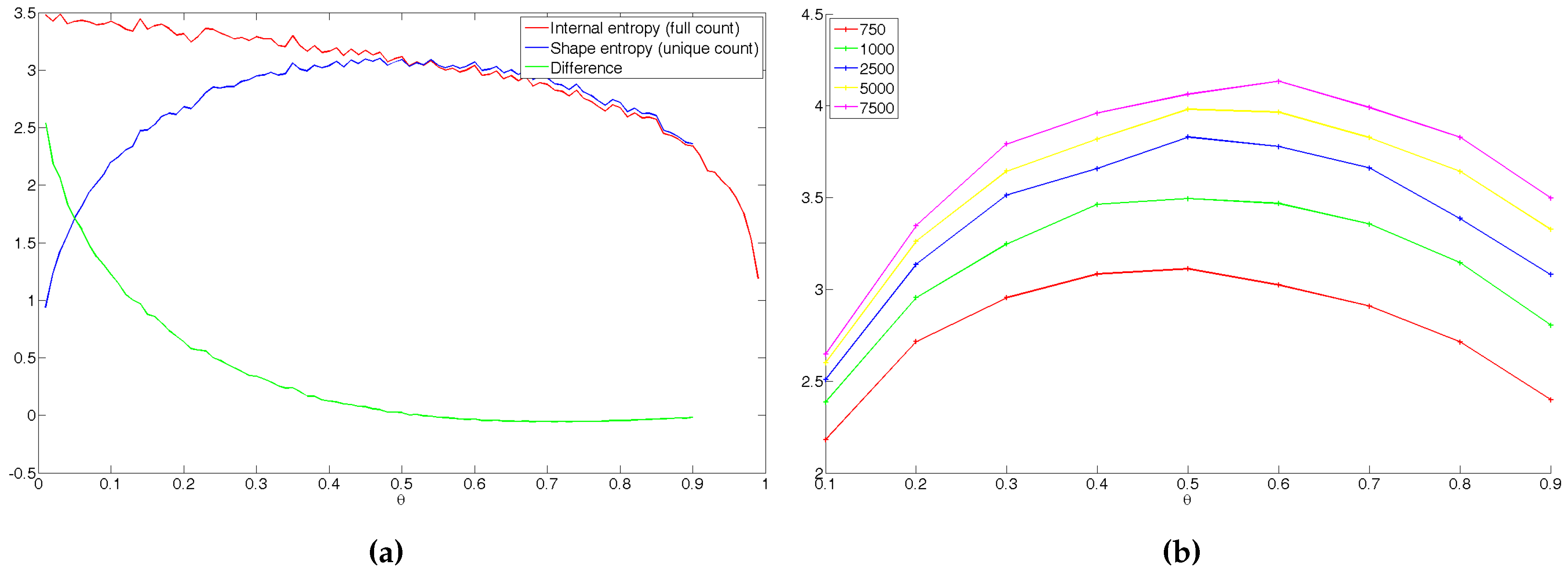
Figure 4. Two Gibbs-Shannon based entropies as functions of θ. The curves are obtained by averaging over 50 correlons for each temperature. (a) Internal and shape entropies as functions of θ and their difference. (b) Shape entropy S_sh as a function of θ for various heat loads N_Q.

Figure 4. Two Gibbs-Shannon based entropies as functions of θ. The curves are obtained by averaging over 50 correlons for each temperature. (a) Internal and shape entropies as functions of θ and their difference. (b) Shape entropy S_sh as a function of θ for various heat loads N_Q.

Let us now discuss the properties of the curves obtained for these entropies (Figure 4a), in the context of our analogy between energy (exergy and anergy) and heat quantum movement. First, the correlon internal entropy tends to a maximum when $\theta \to 0$. This seems fairly intuitive since $\theta \to 0\iff T\to T_0$, which means that the heat quantity represented by the correlon tends to be in thermal equilibrium with its surroundings. The quantum movements are very erratic and exhibit multi-scale details, with increasing complexity as θ decreases.

At high temperature, the correlon shape and internal entropies display the same behaviour and the difference of the two curves tends to 0 as $\theta \to 1$. As a matter of fact, in this limit, the probability $p_{\to }$ tends also to unity, therefore $p_{\mathrm{over}}$ tends to zero so that Equations (8) and (10) tend to the same value. However, as the temperature decreases, there are more and more overlapping movements, and thus less “efficiency” in the quantum movements. In other words, there are more “wasted” displacements, i.e., that have not been exploited to heat a new lattice point. The green curve of Figure 4a shows the difference

$$\delta S=S_{\mathrm{int}}-S_{\mathrm{sh}}$$

(13)

The quantity $\delta S$ may be interpreted as a loss of information from the correlon to the background medium. The shape entropy curve presents a maximum for $\theta =0.5$. It separates the temperature domain in two regions composed of:

• a strongly oriented energy type, efficient to produce work,
• a diffusive form of energy that tends to fill the space.

The value $\theta =0.5$ points out the existence of a particular temperature which appears as an optimal one

$$T_{\mathrm{opt}}=2T_0$$

(14)

which conciliates the two antagonist behaviours previously described and minimizes the information loss from the correlon to the background medium. This optimum is often enhanced in the literature on thermal engine optimisation in the context of finite time thermodynamics. It can be shown that the maximal exergetic power is obtained for an exergetic efficiency of one half, whatever the operating engine (e.g., [18,19]).

Figure 4b displays the shape entropy as a function of θ for different heat quantities. We have not displayed the internal entropy not to overload the graph but for every $N_Q$, it behaves as in Figure 4a, with an increasing maximum when $\theta \to 0$ as $N_Q$ augments. We see that the higher $N_Q\sim Q$ the higher the entropy, which is consistent with Clausius definition of entropy: $dS=\delta Q/T$. All exhibit a wide plateau roughly centred around $\theta =0.5$.

4. Conclusions

We developed a probabilistic toy model based on the main assumption that exergy is the “directed” part of energy, and its complementary (anergy) is the support for exergy. The heat correlons obtained display multi-scale structure with a cut-off length equal to the lattice spacing and an integral length related to the exergy content of the represented heat quantity. We computed their fractal dimensions as functions of θ using two methods:

• the box-counting method gives a dimension related to the overall fractal shape of the correlons, regardless of their internal details;
• the Richardson’s method, sensible to the internal diffusion, allows a characterisation of the overlapping.

The shape fractal dimension may be regarded as a sort of interface fractal dimension. The “loss” of dimensionality with respect to the internal fractal dimension is actually a loss of details. From this interpretation, we adapted the Gibbs–Shannon entropy and proposed two definitions in order to investigate further the impact of overlapping. In considering these movements all together in a single probability $p_{\mathrm{over}}$, the correlon shape entropy as a function of θ, naturally designates an optimal ${\theta }_{\mathrm{opt}}=0.5$ which conciliate between directed exergy flow and supporting anergy content.

References

- Beck, C.; Schlögl, F. Thermodynamics of Chaotic Systems; Cambridge University Press: Cambridge, UK, 1993. [Google Scholar]
- Le Méhauté, A.; Nigmatoullin, R.-R.; Nivanen, L. Flèches du Temps et Géométrie Fractale; Hermes: Paris, France, 1998. (In French) [Google Scholar]
- Gosselin, L.; Bejan, A. Constructal heat trees at micro and nanoscales. J. Appl. Phys. 2004, 96, 5852–5859. [Google Scholar] [CrossRef]
- Bejan, A.; Moran, M.J. Thermal Design and Optimization; Wiley: New York, NY, USA, 1995. [Google Scholar]
- Bejan, A. Constructal-theory network of conducting paths for cooling a heat generating volume. Int. J. Heat Mass Transf. 1997, 40, 799–816. [Google Scholar] [CrossRef]
- Bejan, A. Shape and Structure, from Engineering to Nature; Cambridge University Press: Cambridge, UK, 2000. [Google Scholar]
- Queiros-Conde, D. Le modèle des Peaux Entropiques en Turbulence développée. Comptes Rendus de l’Académie des Sci. 2000, 328, 541–546. (In French) [Google Scholar] [CrossRef]
- Queiros-Condé, D. A diffusion equation to describe scale- and time-dependent dimensions of turbulent interfaces. Proc. Royal Soc. Lond. A Math. Phys. Eng. Sci. 2003, 459, 3043–3059. [Google Scholar] [CrossRef]
- Queiros-Condé, D. Dynamique des Peaux Entropiques Dans les Systèmes Intermittents et Multi-échelles; Habilitation à Diriger des Recherches, Université Henri Poincaré: Nancy, France, 2006. (In French) [Google Scholar]
- Chen, G.Q. Exergy consumption of the earth. Ecol. Model. 2005, 184, 363–380. [Google Scholar] [CrossRef]
- Wu, X.; Chen, G.; Wu, X.; Yang, Q.; Alsaedi, A.; Hayat, T.; Ahmad, B. Renewability and sustainability of biogas system: Cosmic exergy based assessment for a case in China. Renew. Sustain. Energy Rev. 2015, 51, 1509–1524. [Google Scholar] [CrossRef]
- Dincer, I.; Cengel, Y.A. Energy, entropy and exergy concepts and their roles in thermal engineering. Entropy 2001, 3, 116–149. [Google Scholar] [CrossRef]
- Leff, H.S. Entropy, its language, and interpretation. Found. Phys. 2007, 37, 1744–1766. [Google Scholar] [CrossRef]
- Nottale, L.; Chaline, J.; Grou, P. Les Arbres de L’évolution; Hachette: Paris, France, 2000. (In French) [Google Scholar]
- Mandelbrot, B.B. The Fractal Geometry of Nature; W.H. Freeman: New York, NY, USA, 1982. [Google Scholar]
- Lawler, G.F. The dimension of the frontier of planar Brownian motion. Electron. Commun. Probab. 1996, 1, 29–47. [Google Scholar] [CrossRef]
- Queiros-Condé, D.; Chaline, J.; Dubois, J. Le Monde des Fractales—La Nature Trans-échelles; Ellipses: Paris, France, 2015. (In French) [Google Scholar]
- Feidt, M. Thermodynamique et Optimisation Énergétique des Systèmes et Procédés; Technique et Documentation Lavoisier: Paris, France, 1996. (In French) [Google Scholar]
- Neveu, P. Apports de la Thermodynamique Pour la Conception et L’intégration des Procédés. Ph.D. Thesis, Université de Perpignan, Perpignan, France, December 2002. [Google Scholar]
© 2016 by the authors; licensee MDPI, Basel, Switzerland. This article is an open access article distributed under the terms and conditions of the Creative Commons by Attribution (CC-BY) license (http://creativecommons.org/licenses/by/4.0/).
Share and Cite
MDPI and ACS Style
Canivet, Y.; Queiros-Condé, D.; Grosu, L. Fractal Representation of Exergy. Entropy 2016, 18, 56. https://0-doi-org.brum.beds.ac.uk/10.3390/e18020056
AMA Style
Canivet Y, Queiros-Condé D, Grosu L. Fractal Representation of Exergy. Entropy. 2016; 18(2):56. https://0-doi-org.brum.beds.ac.uk/10.3390/e18020056
Chicago/Turabian StyleCanivet, Yvain, Diogo Queiros-Condé, and Lavinia Grosu. 2016. "Fractal Representation of Exergy" Entropy 18, no. 2: 56. https://0-doi-org.brum.beds.ac.uk/10.3390/e18020056
Note that from the first issue of 2016, this journal uses article numbers instead of page numbers. See further details here.