Article

A Memristor-Based Hyperchaotic Complex Lü System and Its Adaptive Complex Generalized Synchronization

1
School of Computer and Information Engineering, Fuyang Normal University, Fuyang 236041, China
2
Faculty of Electronic Information and Electrical Engineering, Dalian University of Technology, Dalian 116024, China
3
College of Electrical Engineering and Automation, Anhui University, Hefei 230601, China
*
Author to whom correspondence should be addressed.
Submission received: 7 December 2015 / Revised: 3 February 2016 / Accepted: 4 February 2016 / Published: 22 February 2016
(This article belongs to the Section Complexity)

Abstract

:
This paper introduces a new memristor-based hyperchaotic complex Lü system (MHCLS) and investigates its adaptive complex generalized synchronization (ACGS). Firstly, the complex system is constructed based on a memristor-based hyperchaotic real Lü system, and its properties are analyzed theoretically. Secondly, its dynamical behaviors, including hyperchaos, chaos, transient phenomena, as well as periodic behaviors, are explored numerically by means of bifurcation diagrams, Lyapunov exponents, phase portraits, and time history diagrams. Thirdly, an adaptive controller and a parameter estimator are proposed to realize complex generalized synchronization and parameter identification of two identical MHCLSs with unknown parameters based on Lyapunov stability theory. Finally, the numerical simulation results of ACGS and its applications to secure communication are presented to verify the feasibility and effectiveness of the proposed method.

1. Introduction

Chaos and hyperchaos can occur in many nonlinear dynamical systems, which can be depicted by time series, phase portraits, Poincare sections, bifurcation diagrams, Lyapunov exponents, fractal dimension, and entropy. The last three parameters in particular are usually used to describe the complexity of chaotic or hyperchaotic systems quantitatively [1,2,3]. Compared to chaotic systems, hyperchaotic systems have a greater randomness and higher complexity and unpredictability, and so they are more suitable and effective for secure communication and digital cryptography. Since Rössler firstly reported hyperchaos in a four-variable oscillator in 1979 [4], hyperchaos has been intensively studied in nonlinear science and technology fields. Hyperchaos can only appear in a no less than fourth-order autonomous nonlinear system, which has at least two positive Lyapunov exponents. Therefore, some hyperchaotic systems were constructed based on three-dimensional chaotic systems [5,6,7,8] by adding a variable and a state feedback item, such as hyperchaotic Lorenz system [9], hyperchaotic Chen system [10], hyperchaotic Lü system [11], hyperchaotic Liu system [12], and so on. It is worth noting that several memristor-based hyperchaotic systems were proposed in recent years. Memristors are considered as the fourth fundamental circuit element with the characteristics of nonlinearity, non-volatility, nanoscale, and low power consumption [13,14,15], and the study of memristors, memristor-based circuits and neural networks have become a key research front in mathematics, computer science and engineering. In [16], hyperchaos was found in a modified canonical Chua’s circuit with a cubic nonlinear memristor by means of numerical simulation and circuit experiment. In [17], hyperchaos and transient hyperchaos were presented in a Murali–Lakshmanan–Chua’s circuit with a three-segment piecewise-linear active flux-controlled memristor. In [18], hyperchaos was investigated in a modified Chua’s circuit with two HP memristors (made by Hewlett-Packard Company, Palo Alto, CA, USA) in antiparallel. In [19], hyperchaos and topological horseshoes were studied in a modified Lü system with a smooth flux-controlled memristor. In [20], a four-wing hyperchaotic attractor was generated from a four-dimensional memristive system with a cubic nonlinear memductance function.
All of the above-mentioned systems are hyperchaotic real systems. However, complex nonlinear systems, i.e., nonlinear systems with complex variables, are more complicated than real systems, and can generate more abundant dynamical behaviors, which can be applied to secure communication for high transmission efficiency and anti-attack ability. Some complex systems, such as complex Lorenz systems [21,22,23], complex Chen systems [24,25], complex Lü systems [26], complex Rössler systems [27], and other complex systems [28,29,30], have been constructed and investigated theoretically and numerically. Among the above literatures, hyperchaotic complex systems were studied in [22,23,24,29]. To our best knowledge, a memristor-based chaotic complex system was firstly introduced in [23], and up to now, there are no reports of memristor-based hyperchaotic complex systems.
It is well known that chaos (hyperchaos) synchronization plays a vital role in nonlinear science and technology, especially for secure communication, digital encryption, signal and control processing [25,31,32,33]. In recent years, some efforts are devoted to achieve various synchronization for complex chaotic and hyperchaotic systems, such as complete synchronization [26,27,28], anti-synchronization [24], lag synchronization [33], projective synchronization [34], phase synchronization [35], combination synchronization [36], and their extended synchronization [29,37,38,39]. In general, adaptive control schemes should be adopted to realize synchronization and parameter identification of complex systems with unknown parameters. In [24], the adaptive synchronization and anti-synchronization problems of a hyperchaotic complex Chen system with unknown parameters was investigated based on passive control. In [40], a novel adaptive modified projective synchronization was introduced for synchronizing two non-identical complex systems with uncertain complex parameters up to a complex scaling matrix. As far as we know, there are no achievements about complex generalized synchronization (CGS) of complex nonlinear systems. However, generalized synchronization (GS), i.e., the response system is synchronized with the drive system with respect to a given functional relationship, is a very flexible synchronization method, which can degenerate to functional projective synchronization (FPS), modified projective synchronization (MPS), projective synchronization (PS), complete synchronization (CS), and anti-synchronization (AS) with different given functions [41,42,43]. Hence, it is meaningful and challenging to extend GS from real systems to complex systems, and to realize ACGS for chaotic and hyperchaotic complex systems with unknown parameters.
Motivated by the above discussions, we firstly construct a memristor-based hyperchaotic complex Lü system (MHCLS) based on a four-dimensional hyperchaotic real Lü system proposed in [19], and investigate its nonlinear properties and dynamical behaviors. Meanwhile, we propose a new synchronization scheme, ACGS, for two identical MHCLSs with unknown parameters based on Lyapunov stability theory, and used it to realize secure transmission of signals and information. The rest of this paper is structured as follows: in Section 2, a novel MHCLS is introduced, and its properties are analyzed theoretically, symmetry and invariance, dissipation, equilibria and stability included. In Section 3, the dynamical behaviors of the system are revealed numerically by means of bifurcation diagram, Lyapunov exponents, time history diagrams, phase portraits. In Section 4, an adaptive controller and a parameter estimator are designed to achieve ACGS and parameter identification for two identical MHCLSs. Furthermore, numerical simulations are presented to demonstrate the proposed scheme and its applications to secure communication. Finally, some concluding remarks are given in Section 5.

2. A New MHCLS and Its Properties

2.1. Generation of MHCLS

In [19], a memristive hyperchaotic real Lü system was firstly constructed by adding a flux-controlled memristor to a traditional Lü system, which can be described by:
{ x ˙ 1 = a 1 ( x 2 x 1 ) x ˙ 2 = x 1 x 3 + a 2 x 2 a 3 W ( x 4 ) x 1 x ˙ 3 = x 1 x 2 a 4 x 3 x ˙ 4 = x 1
where a 1 , a 2 , a 3 , and a 4 are positive parameters, x i R ( i = 1 4 ) , and W ( ) denotes the memductance function of a flux-controlled memristor, which is characterized by a smooth continuous cubic nonlinearity in [15,19] and in this paper:
W ( x 4 ) = a + b x 4 2
where a and b are positive constants. When a = 4 , b = 0.01 , a 1 = 36 , a 2 = 20 , a 4 = 3 , a 3 [ 2.67   3.26 ) , system (1) operates in hyperchaotic state [18]. By substituting complex variables for real variables x 1 , x 2 and keeping the others unchangeable, a complex memristive Lü system is generated as:
{ x ˙ 1 = a 1 ( x 2 x 1 ) x ˙ 2 = x 1 x 3 + a 2 x 2 a 3 ( a + 3 b x 4 2 ) x 1 x ˙ 3 = ( x ¯ 1 x 2 + x 1 x ¯ 2 ) / 2 a 4 x 3 x ˙ 4 = ( x 1 + x ¯ 1 ) / 2
Where x 1 , x 2 C , x 3 , x 4 R , x ¯ 1 , x ¯ 2 C denote the complex conjugate variables of x 1 , x 2 . If x 1 = x 1 , r + j x 1 , i , x 2 = x 2 , r + j x 2 , i , j = 1 , and the subscripts r and i denote the real and image parts of the complex variables, vectors and matrices throughout this paper, complex system (3) can be equivalent to a six real first ordinary differential equations (ODEs):
{ x ˙ 1 , r = a 1 ( x 2 , r x 1 , r ) x ˙ 1 , i = a 1 ( x 2 , i x 1 , i ) x ˙ 2 , r = x 1 , r x 3 + a 2 x 2 , r a 3 ( a + 3 b x 4 2 ) x 1 , r x ˙ 2 , i = x 1 , i x 3 + a 2 x 2 , i a 3 ( a + 3 b x 4 2 ) x 1 , i x ˙ 3 = x 1 , r x 2 , r + x 1 , i x 2 , i a 4 x 3 x ˙ 4 = x 1 , r

2.2. Dissipation of MHCLS

According to the definition of divergence, we calculate the divergence of system (4):
V = x ˙ 1 , r x 1 , r + x ˙ 1 , i x 1 , i + x ˙ 2 , r x 2 , r + x ˙ 2 , i x 2 , i + x ˙ 3 x 3 + x ˙ 4 x 4 = 2 a 1 + 2 a 2 a 3
So, the inequality 2 a 1 + 2 a 2 a 3 < 0 should be satisfied to guarantee that system (4) is dissipative and converges exponentially.

2.3. Symmetry and Invariance of MHCLS

From Equation (4), it is easy to find that the system is invariant under the transformation from ( x 1 , r , x 1 , i , x 2 , r , x 2 , i , x 3 , x 4 ) to ( x 1 , r , x 1 , i , x 2 , r , x 2 , i , x 3 , x 4 ) , ( x 1 , r , x 1 , i , x 2 , r , x 2 , i , x 3 , x 4 ) and ( x 1 , r , x 1 , i , x 2 , r , x 2 , i , x 3 , x 4 ) for any choice of the values of system parameters.

2.4. Equilibria and Stability of MHCLS

By setting the left of six first ODEs to be zero in system (4), i.e., x ˙ 1 , r = 0 , x ˙ 1 , i = 0 , x ˙ 2 , r = 0 , x ˙ 2 , i = 0 , x ˙ 3 = 0 , x ˙ 4 = 0 , and solving them, we can obtain the equilibrium points of system (4):
{ E 1 = { ( x 1 , r , x 1 , i , x 2 , r , x 2 , i , x 3 , x 4 ) | x 1 , r = x 1 , i = x 2 , r = x 2 , i = x 3 = 0 , x 4 = c } E 2 , 3 = { ( x 1 , r , x 1 , i , x 2 , r , x 2 , i , x 3 , x 4 ) | x 1 , r = 0 , x 1 , i = ± p , x 2 , r = 0 , x 2 , i = ± p , x 3 = q , x 4 = c }
where c is an arbitrary real constant, p = a 4 a 2 a 4 a 3 ( a + 3 b c 2 ) , and q = a 2 a 3 ( a + 3 b c 2 ) . There are three line equilibria sets, in which E 1 represents the equilibrium points on x 4 axis, E 2 and E 3 are symmetric, whose stability can be analyzed based on Jacobian matrices and Routh–Hurwitz theorem. The Jacobian matrix of system (4) at E 1 is calculated as:
J E 1 = [ a 1 0 a 1 0 0 0 0 a 1 0 a 1 0 0 a 3 ( a + 3 b c 2 ) 0 a 2 0 0 0 0 a 3 ( a + 3 b c 2 ) 0 a 2 0 0 0 0 0 0 a 4 0 1 0 0 0 0 0 ]
The characteristic polynomial of Equation (7) is:
λ ( λ + a 4 ) ( λ 2 + δ 1 λ + δ 2 ) 2 = 0
where δ 1 = a 1 a 2 , δ 2 = a 1 [ a 3 ( a + 3 b c 2 ) a 2 ) ] . Since a 1 , a 2 , a 3 , a 4 , a , b are positive parameters, Equation (8) has a zero root and a negative root ( a 4 ). If E 1 is stable, it is required that the condition δ 1 > 0 , δ 2 > 0 , i.e., Equation (9), should be satisfied to guarantee the other eigenvalues with negative real parts based on Routh–Hurwitz theorem:
{ a 1 a 2 > 0 a 3 ( a + 3 b c 2 ) a 2 > 0
Due to the symmetry of E 2 and E 3 , we only need to analyze one of them. The Jacobian matrix of system (4) at E 2 is calculated as:
J E 2 = [ a 1 0 a 1 0 0 0 0 a 1 0 a 1 0 0 q a 3 ( a + 3 b c 2 ) 0 a 2 0 0 0 0 q a 3 ( a + 3 b c 2 ) 0 a 2 p 6 a 3 b p c 0 p 0 p a 4 0 1 0 0 0 0 0 ]
The characteristic polynomial of Equation (10) is:
λ 2 ( λ + a 1 a 2 ) ( λ 3 + ω 1 λ 2 + ω 2 λ + ω 3 ) = 0
where ω 1 = a 1 + a 4 a 2 , ω 2 = a 4 [ a 1 a 3 ( a + 3 b c 2 ) ] , ω 3 = 2 a 1 a 4 [ a 2 a 3 ( a + 3 b c 2 ) ] . There are two zero roots and four nonzero roots of Equation (8). According to Routh–Hurwitz theorem, the real parts of the other nonzero roots of Equation (11) are negative if and only if:
a 1 a 2 > 0 , ω 1 > 0 , ω 1 ω 2 ω 3 > 0 , ω 3 ( ω 1 ω 2 ω 3 ) > 0
By substituting ω 1 , ω 2 , ω 3 into Equation (12) and considering positive system parameters a 1 , a 2 , a 3 , a 4 , a , b , the stability condition can be rewritten as:
{ a 1 a 2 > 0 a 2 a 3 ( a + 3 b c 2 ) > 0 ( a 1 + a 4 a 2 ) [ a 1 a 3 ( a + 3 b c 2 ) ] 2 a 1 [ a 2 a 3 ( a + 3 b c 2 ) ] > 0
Apparently, the second conditions of Equations (9) and (13) cannot be satisfied at the same time, so system (4) has unstable equilibrium points with any parameters, which indicates that chaotic and hyperchaotic attractors may occur possibly. By setting a = 4 , b = 0.01 , a 1 = 36 , a 2 = 20 , a 3 = 3.2 , a 4 = 3 , c = 0 , the eigenvalues of the system are calculated as λ E 1 = ( 0 , 25.88 , 9.88 , 9.88 , 25.88 , 3 ) , λ E 2 = λ E 3 = ( 16 , 19.48 , 0.24 + 8.87 j , 0.24 8.87 j , 0 , 0 ) , which indicate E 1 , E 2 and E 3 are all unstable.

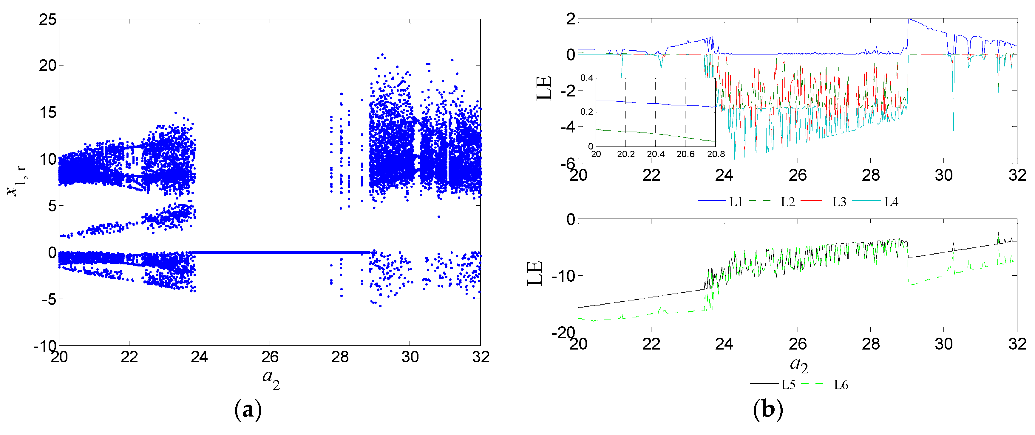
3. Dynamical Behaviors of MHCLS

In order to explore the dynamical behaviors of MHCLS with different parameter values, we set a = 4 , b = 0.01 , a 1 = 36 , a 3 = 3.2 , a 4 = 3 , x 0 = ( 1 + 2 j , 1 + j , 2 , 1 ) and vary a 2 in range of [ 20 , 32 ] . As introduced in [23,44,45], transient phenomena can appear in some memristor-based nonlinear systems, which need much longer computational time to achieve the steady states of the system. Hence, we use ode45 solver of Matlab® R2013a to simulate the system for plotting bifurcation diagram and calculating Lyapunov exponents with computational time interval 0–20,000 s and 0–100,000 s separately. As shown in Figure 1, the bifurcation diagram and Lyapunov exponent spectrum consistently display the dynamical evolution process of the system with different parameter values. The dynamical behaviors of the system are associated with the number of the positive Lyapunov exponents. The system operates in periodic state when all of the six exponents are not greater than zero and in chaotic state when one positive Lyapunov exponent exists. In particular, there are two positive Lyapunov exponents for a 2 [ 20 , 20.8 ] , as shown in the inserted sub-figure of Figure 1b, which indicate hyperchaos occurs in such range. Specifically, some conventional numerical methods are utilized to describe the dynamical behaviors in detail as shown in Figure 2, Figure 3, Figure 4 and Figure 5.
Figure 1. (a) Bifurcation diagram; (b) Lyapunov exponent spectrum.
Entropy 18 00058 g001

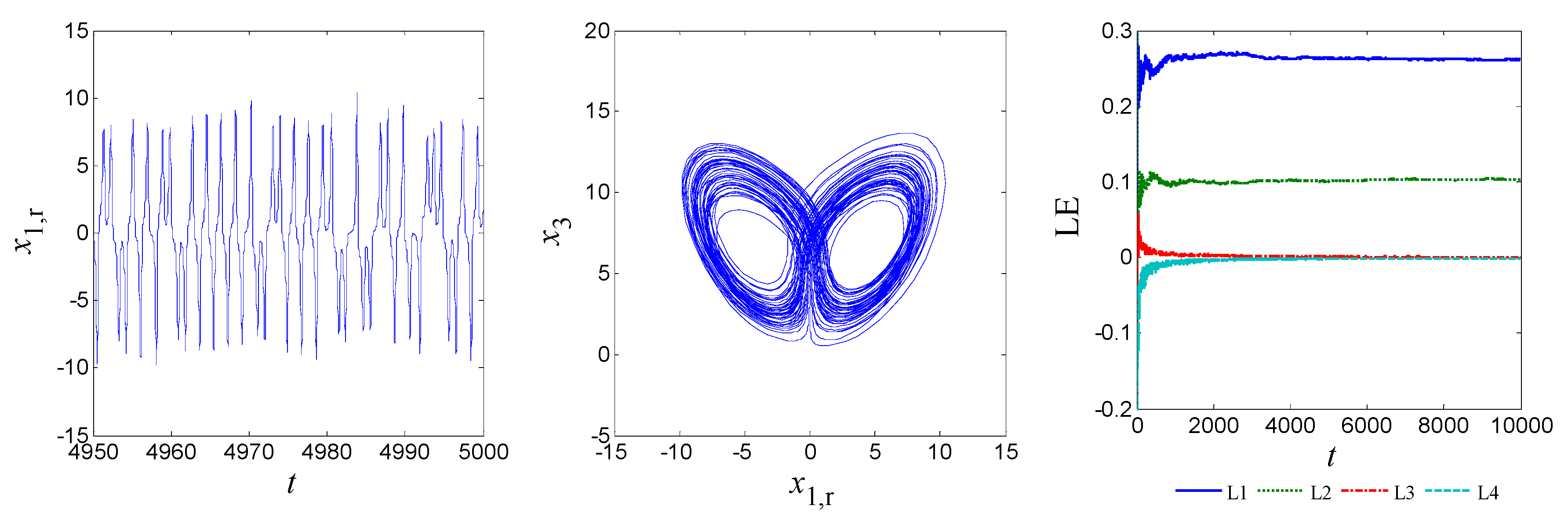
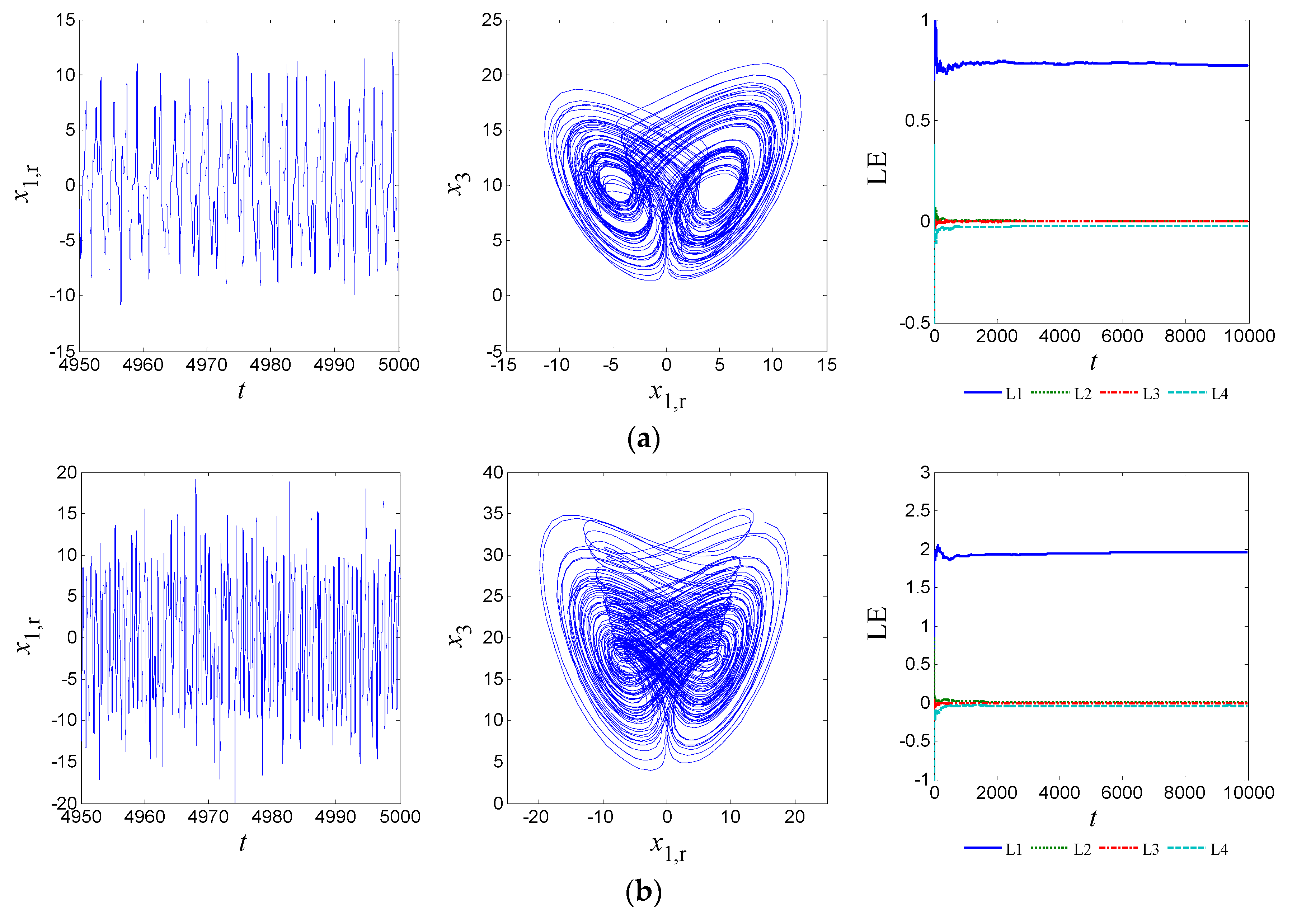
3.1. Hyperchaotic Behavior

When a 2 = 20 , there are two positive Lyapunov exponents, and a butterfly-shape hyperchaotic attractor occurs which is similar to the Lorenz attractor, as shown in Figure 2. It is necessary to note that two negative Lyapunov exponents (i.e., L5, L6) are omitted in Figure 2, Figure 3, Figure 4 and Figure 5, which makes no influence on the analytical results.
Figure 2. Hyperchaotic behavior ( a 2 = 20 ).
Entropy 18 00058 g002

3.2. Chaotic Behavior

The system operates chaotically with one positive Lyapunov exponent as shown in Figure 3. It is interesting to note that the system has chaotic attractors with different shapes. For example, a chaotic attractor has transitory shape between the Lorenz attractor and Chen attractor for a 2 = 23 , while another chaotic attractor is similar to the Chen attractor for a 2 = 29 .
Figure 3. Chaotic behavior. (a) Chaos ( a 2 = 23 ); (b) Chaos ( a 2 = 29 ).
Entropy 18 00058 g003
Figure 4. Periodic behavior. (a) Period-3 ( a 2 = 21.92 ); (b) Period-2 ( a 2 = 31.1 ).
Entropy 18 00058 g004
Figure 5. Transient behavior. (a) Transient chaos to Period-5 ( a 2 = 21.15 ); (b) Transient chaos to Period-3 orbit ( a 2 = 30.19 ).
Entropy 18 00058 g005

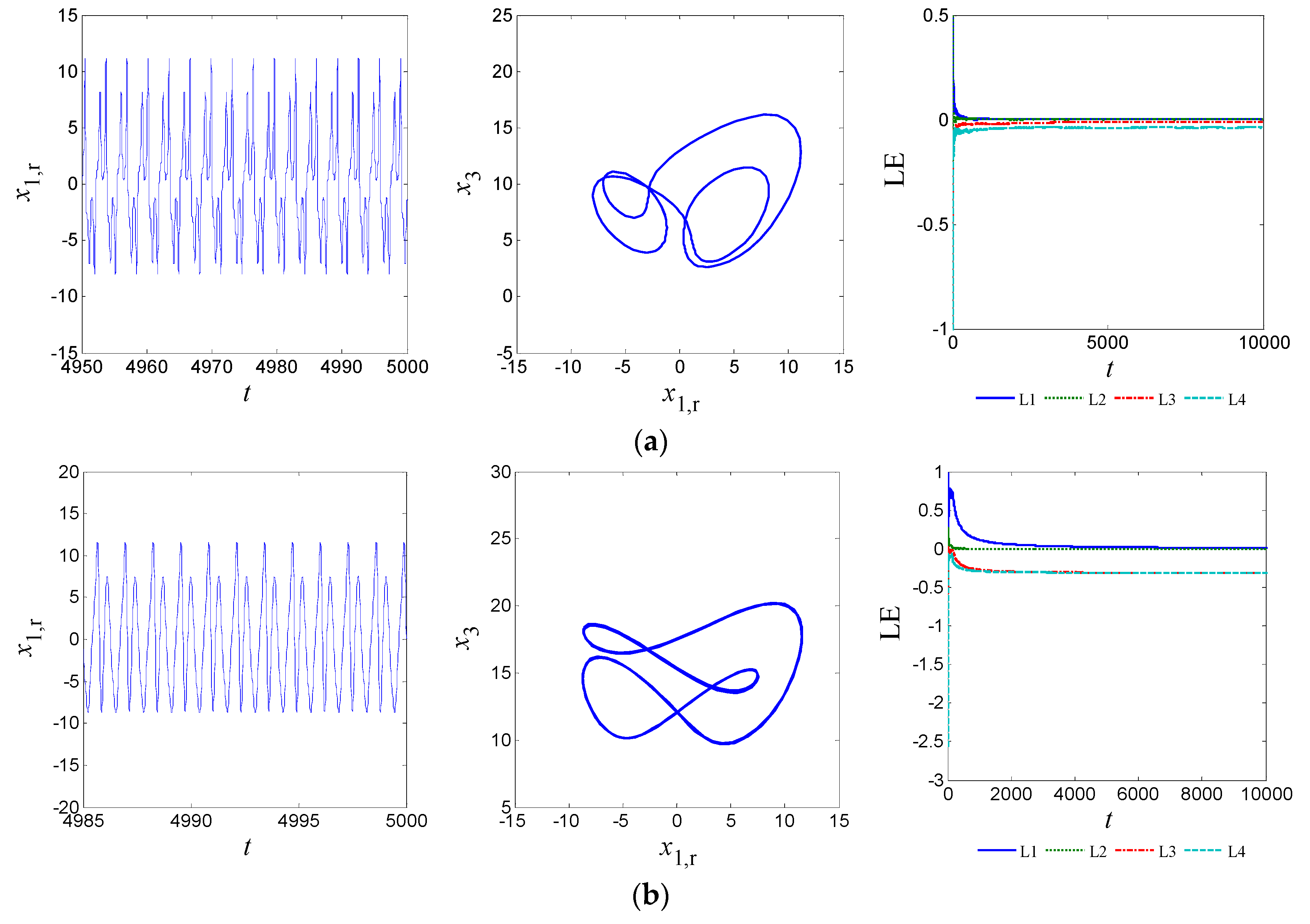
3.3. Periodic Behavior

As shown in Figure 4, the system operates in Period-3 orbit for a 2 = 21.92 and Period-2 orbit for a 2 = 31.1 , and all of the corresponding Lyapunov exponents are not greater than zero.

3.4. Transient Behavior

The system goes through transient chaos, and then enters into the state of Period-5 for a 2 = 21.15 and Period-3 for a 2 = 30.19 , as shown in Figure 5a,b respectively. The Lyapunov exponent L1 is positive in the beginning, and then tends to zero asymptotically and slowly. The inserted sub-figures in red of the time history diagrams and phase portraits belong to transient states.

4. ACGS of Two Identical MHCLSs with Unknown Parameters

4.1. Design of ACGS

Consider the following identical drive and response complex systems:
x ˙ = F ( x ) θ + f ( x )
y ˙ = F ( y ) θ ^ + f ( y ) + u ( x , y )
where x = [ x 1 , x 2 , x n ] T C n is a state complex vector of the drive system (14), and x = x r + j x i . y = [ y 1 , y 2 , y n ] T C n is a state complex vector of the response system (15), and y = y r + j y i . θ R m is a parameter vector of system (14), θ ^ R m is a parameter vector of system (15) which denotes the estimation of θ . F ( ) is an n × m complex matrix whose elements are functions of state complex variables, and F ( ) = F r ( ) + j F i ( ) . f ( ) = [ f 1 , f 2 , f n ] T C n is a vector of complex functions, and f ( ) = f r ( ) + j f i ( ) . u ( x , y ) = [ u 1 , u 2 , u n ] T C n is a control vector of system (15), and u ( x , y ) = u r + j u i . Define the synchronization error:
e ( t ) = y ϕ ( x )
where e ( t ) = [ e 1 , e 2 , e n ] T C n is an error complex vector between systems (14) and (15), and e ( t ) = e r ( t ) + j e i ( t ) . ϕ ( x ) = [ ϕ 1 , ϕ 2 , ϕ n ] T C n is a nonzero map complex vector whose elements are continuous map complex functions, and ϕ ( x ) = ϕ r ( x ) + j ϕ i ( x ) .
Definition 1.  
The response system (14) is complex generalized synchronized with the drive system (15) with respect to the complex vector map ϕ , if there exist a controller u ( x , y ) C n and a given complex map ϕ : C n C n such that the following property is satisfied:
lim t e ( t ) = lim t y ϕ ( x ) = 0
By differentiating Equation (16), the synchronization error dynamical system can be obtained:
e ˙ ( t ) = y ˙ J ( ϕ ) x ˙
where J ( ϕ ) C n × n is the Jacobian matrix of ϕ ( x ) , and J ( ϕ ) = J r ( ϕ ) + j J i ( ϕ ) . By substituting Equations (14) and (15) into Equation (18), we can get:
e ˙ ( t ) = [ F ( y ) J ( ϕ ) F ( x ) ] θ ^ + J ( ϕ ) F ( x ) θ ˜ + f ( y ) J ( ϕ ) f ( x ) + u ( x , y ) = { [ F r ( y ) J r ( ϕ ) F r ( x ) + J i ( ϕ ) F i ( x ) ] θ ^ + [ J r ( ϕ ) F r ( x ) J i ( ϕ ) F i ( x ) ] θ ˜ + f r ( y ) J r ( ϕ ) f r ( x ) + J i ( ϕ ) f i ( x ) + u r ( x , y ) } + j { [ F i ( y ) J r ( ϕ ) F i ( x ) J i ( ϕ ) F r ( x ) ] θ ^ + [ J r ( ϕ ) F i ( x ) + J i ( ϕ ) F r ( x ) ] θ ˜ + f i ( y ) J r ( ϕ ) f i ( x ) J i ( ϕ ) f r ( x ) + u i ( x , y ) }
where θ ˜ = θ ^ θ is the error between the estimated value θ ^ and the true value θ .
Theorem 1. 
For the given map complex vector ϕ ( x ) , the response system (15) can be synchronized with the drive system (14) asymptotically, if the complex adaptive controller and update laws of the real parameters are designed as:
u ( x , y ) = [ F ( y ) J ( ϕ ) F ( x ) ] θ ^ f ( y ) + J ( ϕ ) f ( x ) K e ( t ) = { [ F r ( y ) J r ( ϕ ) F r ( x ) + J i ( ϕ ) F i ( x ) ] θ ^ f r ( y ) + J r ( ϕ ) f r ( x ) J i ( ϕ ) f i ( x ) K e r ( t ) } + j { [ F i ( y ) J r ( ϕ ) F i ( x ) J i ( ϕ ) F r ( x ) ] θ ^ f i ( y ) + J r ( ϕ ) f i ( x ) + J i ( ϕ ) f r ( x ) K e i ( t ) }
θ ˜ ˙ = θ ^ ˙ = k θ [ J ( ϕ ) F ( x ) ] T e ( t ) = K θ { J r ( ϕ ) F r ( x ) J i ( ϕ ) F i ( x ) ] T e r ( t ) + J r ( ϕ ) F i ( x ) + J i ( ϕ ) F r ( x ) ] T e i ( t ) }
where K = d i a g ( k 1 , k 2 , k n ) is the control gain, and K θ = d i a g ( k θ 1 , k θ 2 , k θ m ) is the parameter gain, whose elements are all real positive constants.
Proof. 
Choosing the Lyapunov function as:
V ( t ) = 1 2 ( e r T e r + e i T e i + k θ 1 θ ˜ T θ ˜ )
The time derivative of V ( t ) along the trajectories of the error system (19) is:
V ˙ ( t ) = e ˙ r T e r + e ˙ i T e i + k θ 1 θ ˜ T θ ˜ ˙ = { [ F r ( y ) J r ( ϕ ) F r ( x ) + J i ( ϕ ) F i ( x ) ] θ ^ + [ J r ( ϕ ) F r ( x ) J i ( ϕ ) F i ( x ) ] θ ˜ + f r ( y ) J r ( ϕ ) f r ( x ) + J i ( ϕ ) f i ( x ) + u r ( x , y ) } T e r + { [ F i ( y ) J r ( ϕ ) F i ( x ) J i ( ϕ ) F r ( x ) ] θ ^ + [ J r ( ϕ ) F i ( x ) + J i ( ϕ ) F r ( x ) ] θ ˜ + f i ( y ) J r ( ϕ ) f i ( x ) J i ( ϕ ) f r ( x ) + u i ( x , y ) } T e i k θ 1 θ ˜ T k θ { J r ( ϕ ) F r ( x ) J i ( ϕ ) F i ( x ) ] T e r + J r ( ϕ ) F i ( x ) + J i ( ϕ ) F r ( x ) ] T e i }
Substituting Equations (20) and (21) into Equation (23), then:
V ˙ ( t ) = { [ J r ( ϕ ) F r ( x ) J i ( ϕ ) F i ( x ) ] θ ˜ K e r } T e r + { [ J r ( ϕ ) F i ( x ) + J i ( ϕ ) F r ( x ) ] θ ˜ K e i } T e i θ ˜ T { J r ( ϕ ) F r ( x ) J i ( ϕ ) F i ( x ) ] T e r + J r ( ϕ ) F i ( x ) + J i ( ϕ ) F r ( x ) ] T e i } = e r T K T e r e i T K T e i = e r T K e r e i T K e i < 0
Since V ( t ) is a positive Lyapunov function, and its derivative V ˙ ( t ) is negative, according to the Lyapunov stability theorem, the errors, e r ( t ) 0 , e i ( t ) 0 and θ ˜ 0 as t 0 . Hence, the ACGS of systems (14) and (15) is accomplished. □

4.2. ACGS of Two Identical MHCLSs

The system (3) is chosen as the drive system, and the response system is defined as:
{ y ˙ 1 = a ^ 1 ( y 2 y 1 ) + u 1 y ˙ 2 = y 1 y 3 + a ^ 2 y 2 a ^ 3 ( a + 3 b y 4 2 ) y 1 + u 2 y ˙ 3 = ( y ¯ 1 y 2 + y 1 y ¯ 2 ) / 2 a ^ 4 y 3 + u 3 y ˙ 4 = ( y 1 + y ¯ 1 ) / 2 + u 4
where y 1 , y 2 C , y 3 , y 4 R , y ¯ 1 , y ¯ 2 C denote the complex conjugate variables of y 1 , y 2 , a ^ 1 , a ^ 2 , a ^ 3 , a ^ 4 are the estimated values of unknown parameters a 1 , a 2 , a 3 , a 4 , a , b are considered as the known positive constants, and u 1 , u 2 , u 3 , u 4 denote the controllers. The drive system (3) and response system (25) can be rewritten as the form of systems (14) and (15), where:
F ( x ) = [ x 2 x 1 0 0 0 0 x 2 ( a + 3 b x 4 2 ) x 1 0 0 0 0 x 3 0 0 0 0 ] , f ( x ) = [ 0 x 1 x 3 ( x 1 x ¯ 2 + x ¯ 1 x 2 ) / 2 ( x 1 + x ¯ 1 ) / 2 ] , θ = [ a 1 a 2 a 3 a 4 ]
F ( y ) = [ y 2 , y 1 0 0 0 0 y 2 ( a + 3 b y 4 2 ) y 1 0 0 0 0 y 3 0 0 0 0 ] , f ( y ) = [ 0 y 1 y 3 ( y 1 y ¯ 2 + y ¯ 1 y 2 ) / 2 ( y 1 + y ¯ 1 ) / 2 ] , θ ^ = [ a ^ 1 a ^ 2 a ^ 3 a ^ 4 ] , u = [ u 1 u 2 u 3 u 4 ]
The map complex vector is given by:
ϕ ( x ) = [ ( 1 + j ) x 1 , 2 x 2 , x 3 + x 4 , x 4 2 ] T
The Jacobian matrix of the map ϕ ( x ) is calculated as:
J ( ϕ ) = [ 1 + j 0 0 0 0 2 0 0 0 0 1 1 0 0 0 2 x 4 ]
According to Equations (20) and (21), the complex adaptive controller and update laws of the unknown parameters can be designed as:
{ u 1 , r = ( y 2 , r y 1 , r x 2 , r + x 2 , i + x 1 , r x 1 , i ) a ^ 1 k 1 e 1 , r u 1 , i = ( y 2 , i y 1 , i x 2 , i + x 1 , i x 2 , r + x 1 , r ) a ^ 1 k 1 e 1 , i u 2 , r = ( y 2 , r 2 x 2 , r ) a ^ 2 + [ ( a + 3 b y 4 2 ) y 1 , r 2 ( a + 3 b x 4 2 ) x 1 , r ] a ^ 3 + y 1 , r y 3 2 x 1 , r x 3 k 2 e 2 , r u 2 , i = ( y 2 , i 2 x 2 , i ) a ^ 2 + [ ( a + 3 b y 4 2 ) y 1 , i 2 ( a + 3 b x 4 2 ) x 1 , i ] a ^ 3 + y 1 , i y 3 2 x 1 , i x 3 k 2 e 2 , i u 3 = ( y 3 x 3 ) a ^ 4 y 1 , r y 2 , r y 1 , i y 2 , i + x 1 , r x 2 , r + x 1 , i x 2 , i + x 1 , r k 3 e 3 u 4 = 2 x 1 , r x 4 y 1 , r k 4 e 4
{ a ^ ˙ 1 = k θ 1 [ ( x 2 , r x 1 , r x 2 , i + x 1 , i ) e 1 , r + ( x 2 , i x 1 , i + x 2 , r x 1 , r ) e 1 , i ] a ^ ˙ 2 = k θ 2 ( 2 x 2 , r e 2 , r + 2 x 2 , i e 2 , i ) a ^ ˙ 3 = k θ 3 [ 2 ( a + 3 b x 4 2 ) x 1 , r e 2 , r 2 ( a + 3 b x 4 2 ) x 1 , i e 2 , i ] a ^ ˙ 4 = k θ 4 ( x 3 e 3 )
where e 1 , r = y 1 , r x 1 , r + x 1 , i , e 1 , i = y 1 , i x 1 , r x 1 , i , e 2 , r = y 2 , r 2 x 2 , r , e 2 , i = y 2 , i 2 x 2 , i , e 3 = y 3 x 3 x 4 , e 4 = y 4 x 4 2

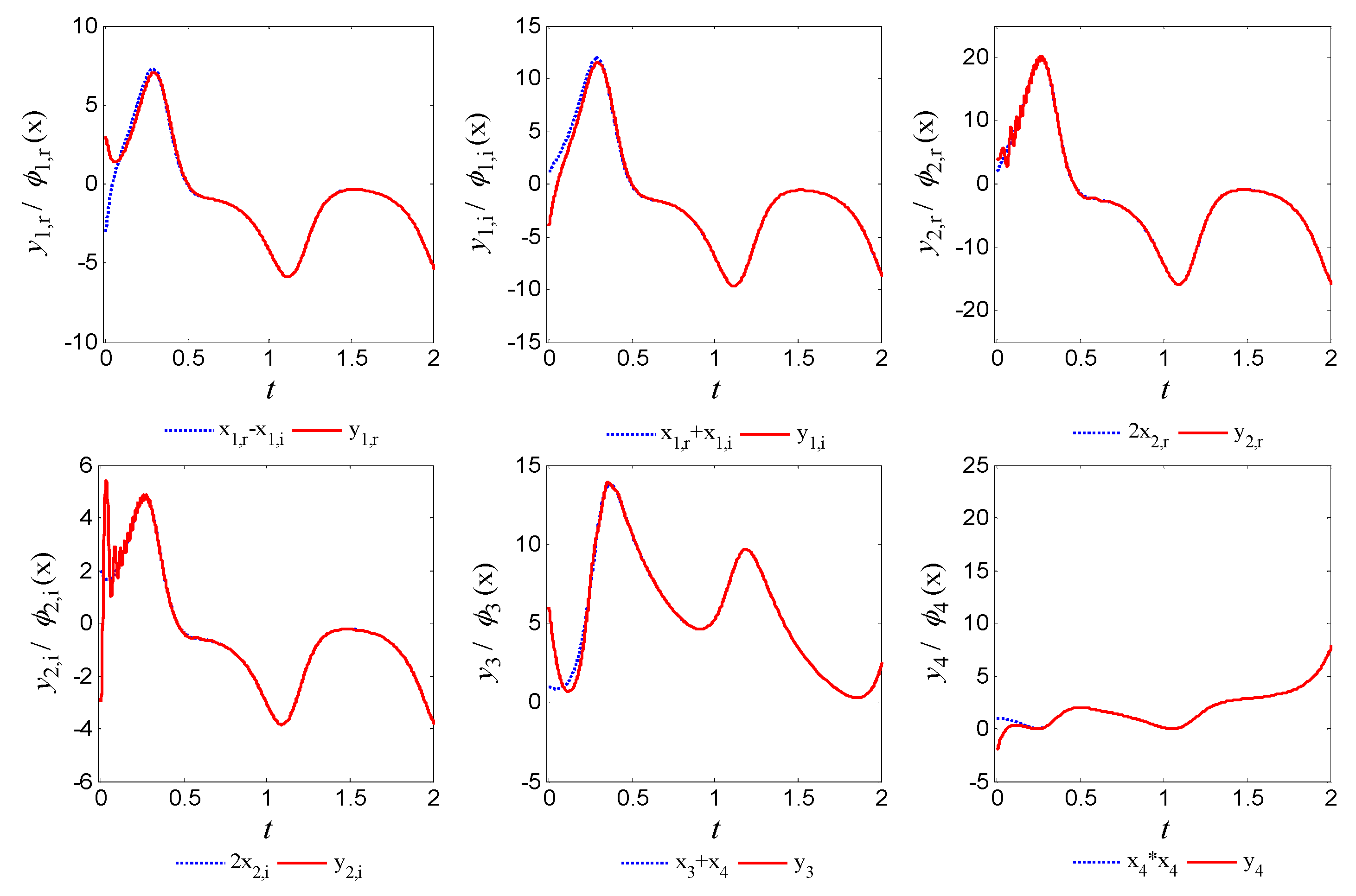
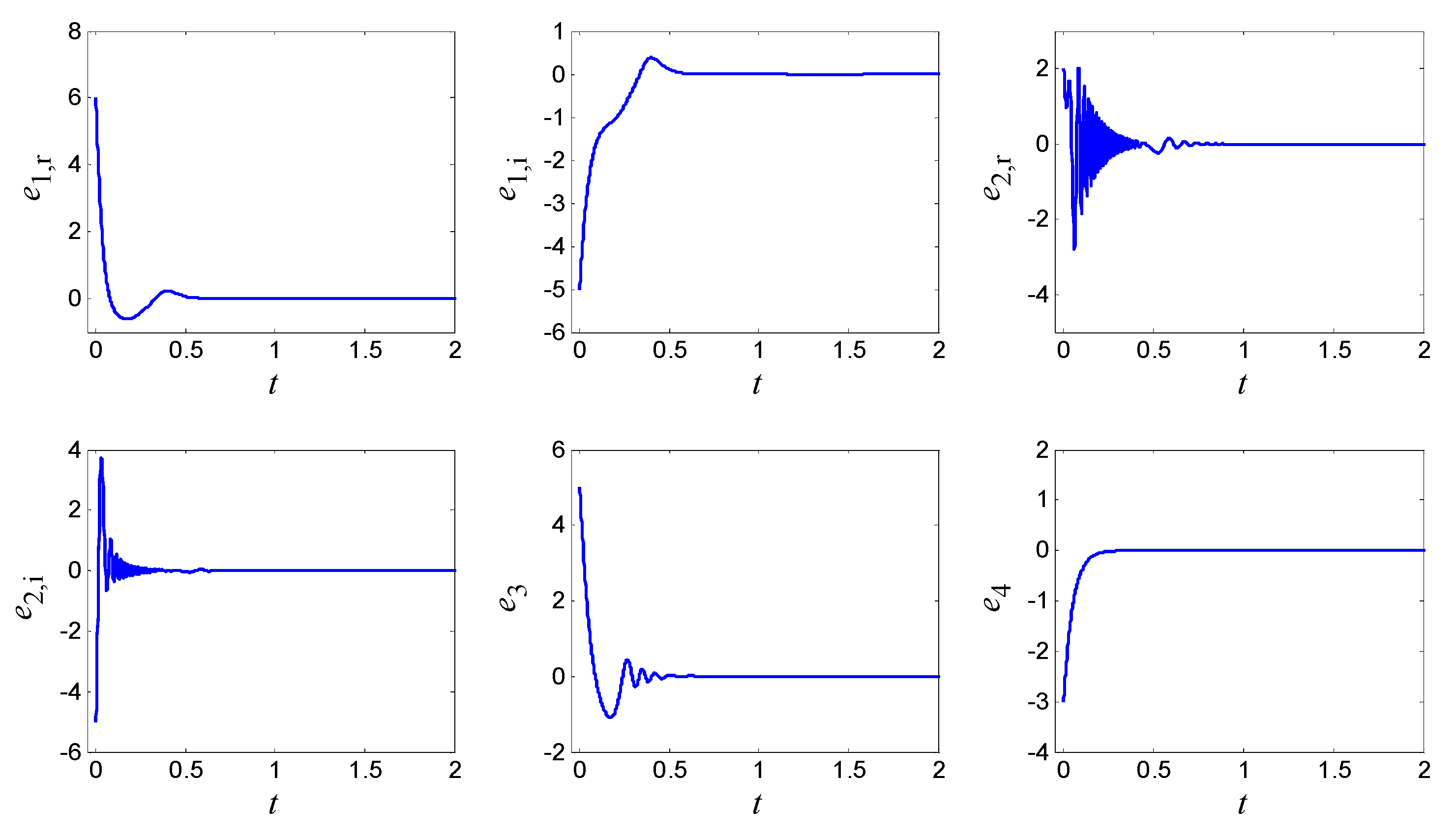
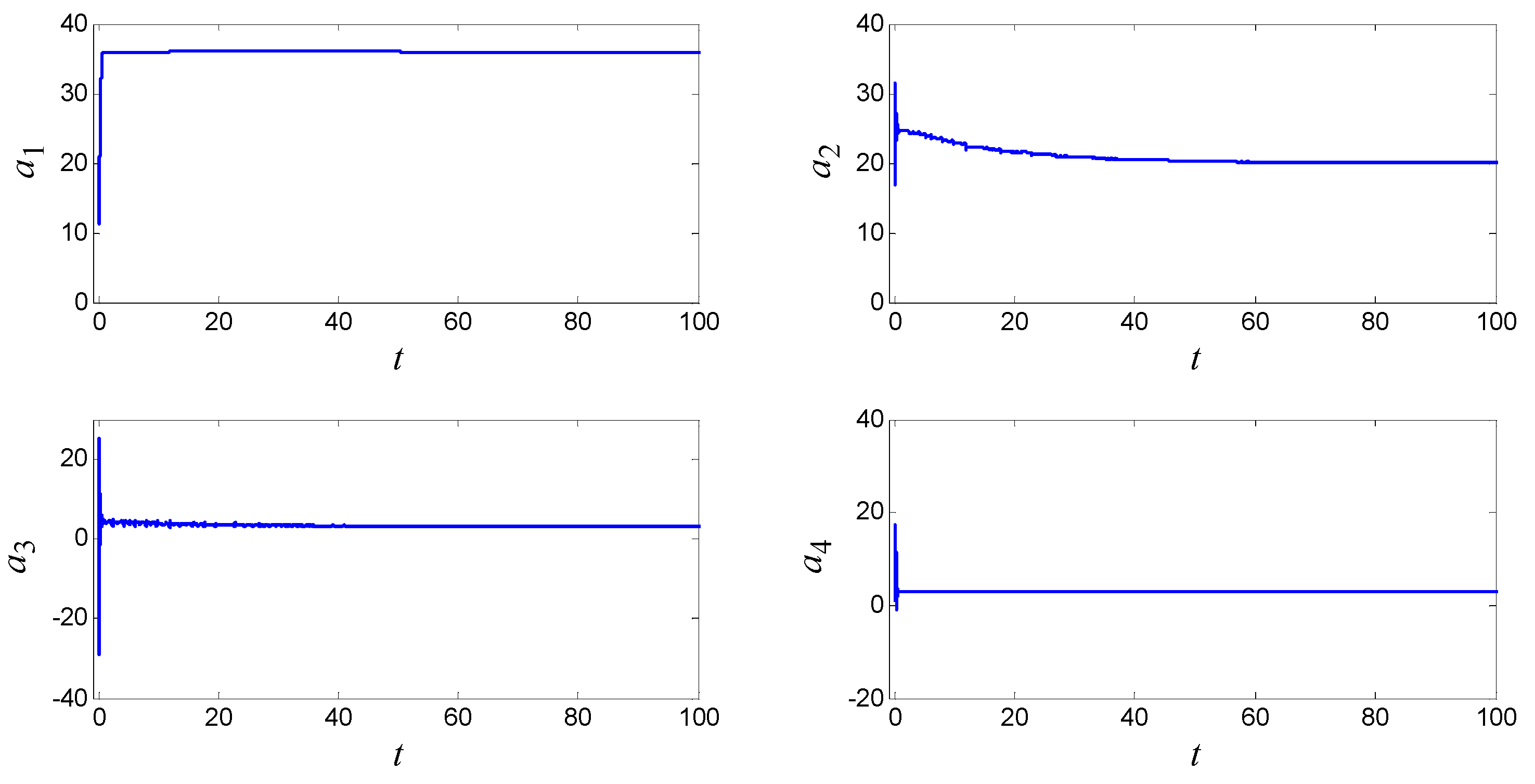
4.3. Numerical Simulations of ACGS

In order to verify the validity and effectiveness of the above-mentioned ACGS scheme, we choose Equation (26) as the map complex vector, and set the values of parameters and initial conditions as: a = 4 , b = 0.01 , a 1 = 36 , a 2 = 20 , a 3 = 3.2 , a 4 = 3 , a ^ 1 = 20 , a ^ 2 = 30 , a ^ 3 = 5 , a ^ 4 = 1 , x 0 = ( 1 + 2 j , 1 + j , 2 , 1 ) T , y 0 = ( 3 4 j , 4 3 j , 6 , 2 ) T , k i = 20 , k θ i = 50 ( i = 1 4 ) . The simulation results are illustrated in Figure 6, Figure 7 and Figure 8, which consistently indicate that ACGS and parameters identification of two identical MHCLSs are realized successively. In detail, time history diagrams of the response system (25) and the map complex functions (26) are plotted in Figure 6, which shows the response system (25) is synchronized with the drive system (3) with respect to the map complex vector (26). Figure 7 shows that the complex generalized synchronization errors asymptotically converge to zero within a second. In Figure 8, the estimated values of unknown parameters converge to a ^ 1 = 36 , a ^ 2 = 20 , a ^ 3 = 3.2 , a ^ 4 = 3 , which indicates the parameter identification of the unknown parameters of drive system is achieved.
Figure 6. The time histories of the drive system (3) and response system (25).
Entropy 18 00058 g006
Figure 7. ACGS errors between the drive system (3) and response system (25).
Entropy 18 00058 g007
Figure 8. The identification process of unknown parameters.
Entropy 18 00058 g008

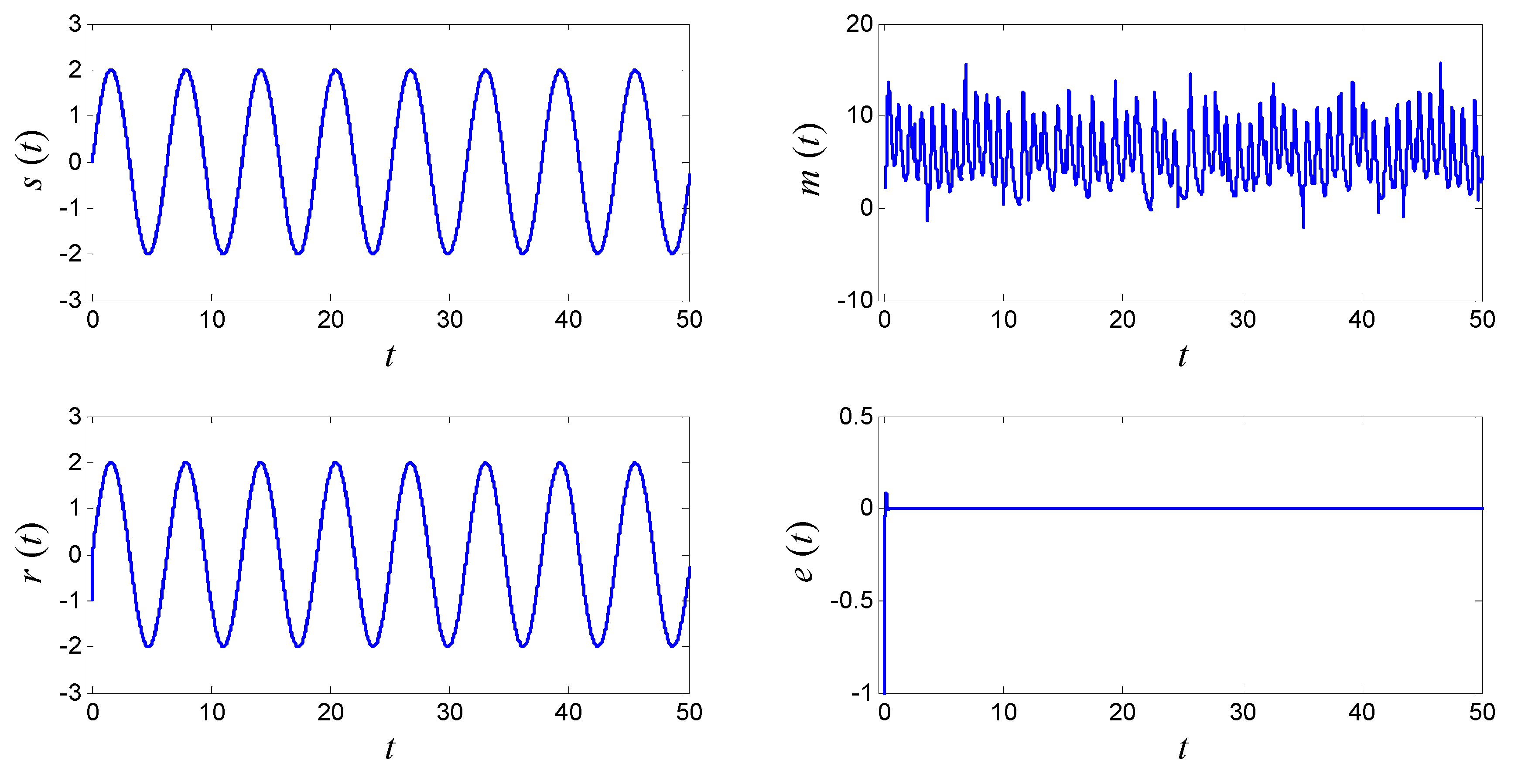
4.4. The Application of ACGS to Secure Communication

In this section, secure communication is investigated based on ACGS of two identical MHCLSs. The drive system (3) and response system (25) are considered as the transmitter and receiver of communication, respectively. The original message signal s ( t ) is transformed by means of an invertible function φ ( ) , and then added to one of the variables for chaotic encryption, which forms the combined signal m ( t ) . The transmitter sends its own hyperchaotic signals and the combined signal to the receiver through communication channels. At the receiver side, the response system can be synchronized with the drive system with respect to the given complex map vector after a short-time transient fluctuation. Based on ACGS, the hyperchaotic part of the combined signal can be filtered out, and then the recovered message signal r ( t ) can be obtained through an inverse transformation φ 1 ( ) .
Figure 9. Secure communication based on AGCS.
Entropy 18 00058 g009
In order to realize secure communication by numerical simulations, all of the parameters and initial conditions are set as those in the sub-section 4.3. The original signal is chosen as s ( t ) = 2 sin t , and invertible function as φ ( ) = arctanh ( ) , i.e., the hyperbolic arctangent function. The transformed signal is assumed to be added to the variable x 3 , and then the combined signal can be described as m ( t ) = arctanh ( s ( t ) ) + x 3 . The simulation result is shown in Figure 9, wherein the original signal s ( t ) , the combined signal m ( t ) , the recovered signal r ( t ) , and the error e ( t ) = r ( t ) s ( t ) are depicted respectively. It is obvious that the original signal is encrypted and recovered successfully.

5. Conclusions

This paper introduces a new memristor-based hyperchaotic complex Lü system, and analyzes its properties and dynamical behaviors theoretically and numerically, which indicate that the system has three line sets of equilibrium points and can generate abundant behaviors, such as periodic operations, transient phenomena, hyperchaotic and chaotic attractors with different shapes. Furthermore, generalized synchronization is extend from real systems to complex systems, and an adaptive complex generalized synchronization controller and a parameter estimator are proposed to synchronize two identical hyperchaotic complex systems with unknown parameters. The corresponding simulation results agree well with the proposed scheme, and demonstrate that the response MHCLS is synchronized with the drive MHCLS with respect to a given complex functional relationship, and the identification of unknown parameters is achieved successfully. The proposed ACGS method is not only used for synchronizing identical MHCLSs, but also used for synchronizing any identical chaotic or hyperchaotic complex systems with unknown parameters, which can be applied to secure communication for higher secure performance and transmission efficiency due to its complex variables, unknown parameters and unpredictable map complex vector.

Acknowledgments

This work was supported by National Natural Science Foundation of China [61370145, 61173183, and 61071023], the Natural Science Foundation of Anhui Provincial Universities [KJ2012A214, KJ2011ZD07], Program for Liaoning Excellent Talents in University [LR2012003], and National Statistical Science Research Project of China [2014LZ32].

Author Contributions

Shibing Wang, Xingyuan Wang, and Yufei Zhou collectively realized nonlinear analyses of MHCLS and designed ACGS theoretically; Shibing Wang and Bo Han performed numerical simulations of all figures; Shibing Wang wrote the paper. All authors have read and approved the manuscript.

Conflicts of Interest

The authors declare no conflict of interest.

References

  1. Geisel, T. Chaos, randomness and dimension. Nature 1982, 298, 322–323. [Google Scholar] [CrossRef]
  2. Chaudhuri, J.R. Chaos and information entropy production. J. Phys. A 2000, 33, 8331–8350. [Google Scholar]
  3. Wolf, A.; Swift, J.B.; Swinney, H.L.; Vastano, J.A. Determining Lyapunov exponents from a series. Phys. D 1985, 16, 285–317. [Google Scholar] [CrossRef]
  4. Rössler, O.E. An equation for hyperchaos. Phys. Lett. A 1979, 71, 155–157. [Google Scholar] [CrossRef]
  5. Lorenz, E.N. Deterministic nonperiodic flow. J. Atmos. Sci. 1963, 20, 130–141. [Google Scholar] [CrossRef]
  6. Chen, G.; Ueta, T. Yet another chaotic attractor. Int. J. Bifurc. Chaos 1999, 9, 1465–1466. [Google Scholar] [CrossRef]
  7. Lü, J.; Chen, G. A new chaotic attractor coined. Int. J. Bifurc. Chaos 2002, 12, 659–661. [Google Scholar] [CrossRef]
  8. Liu, C.; Liu, T.; Liu, L.; Liu, K. A new chaotic attractor. Chaos Solitons Fractals 2004, 22, 1031–1038. [Google Scholar] [CrossRef]
  9. Wang, X.; Wang, M. A hyperchaos generated from Lorenz system. Phys. A 2008, 387, 3751–3758. [Google Scholar] [CrossRef]
  10. Gao, T.; Gu, Q.; Chen, Z. Analysis of the hyper-chaos generated from Chen’s system. Chaos Solitons Fractals 2009, 39, 1849–1855. [Google Scholar] [CrossRef]
  11. Wang, G.; Zhang, X.; Zheng, Y.; Li, Y. A new modified hyperchaotic Lü system. Phys. A 2006, 371, 260–272. [Google Scholar] [CrossRef]
  12. Liu, C. A new hyperchaotic dynamical system. Chin. Phys. 2007, 16, 3279–3284. [Google Scholar]
  13. Chua, L.O. Memristor—The missing circuit element. IEEE Trans. Circuit Theory 1971, 18, 507–519. [Google Scholar] [CrossRef]
  14. Strukov, D.B.; Snider, G.S.; Stewart, D.R.; Williams, R.S. The missing memristor found. Nature 2008, 453, 80–83. [Google Scholar] [CrossRef] [PubMed]
  15. Itoh, M.; Chua, L.O. Memristor Oscillators. Int. J. Bifurc. Chaos 2008, 18, 3183–3206. [Google Scholar] [CrossRef]
  16. Fitch, A.L.; Yu, D.; Iu, H.H.C.; Sreeram, V. Hyperchaos in a memristor-based modified canonical Chua’s circuit. Int. J. Bifurc. Chaos 2012, 22. [Google Scholar] [CrossRef]
  17. Ishaq Ahamed, A.; Lakshmanan, M. Nonsmooth bifurcations, transient hyperchaos and hyper-chaotic beats in a memristive Murali-Lakshmanan-Chua circuit. Int. J. Bifurc. Chaos 2013, 23. [Google Scholar] [CrossRef]
  18. Buscarino, A.; Fortuna, L.; Frasca, M.; Gambuzza, L.V. A gallery of chaotic oscillators based on HP memristor. Int. J. Bifurc. Chaos 2013, 23. [Google Scholar] [CrossRef]
  19. Li, Q.; Zeng, H.; Li, J. Hyperchaos in a 4D memristive circuit with infinitely many stable equilibria. Nonlinear Dyn. 2015, 79, 2295–2308. [Google Scholar] [CrossRef]
  20. Ma, J.; Chen, Z.; Wang, Z.; Zhang, Q. A four-wing hyper-chaotic attractor generated from a 4-D memristive system with a line equilibrium. Nonlinear Dyn. 2015, 81, 1275–1288. [Google Scholar] [CrossRef]
  21. Fowler, A.C.; Gibbon, J.D.; Mcguinness, M.J. The complex Lorenz equations. Phys. D 1982, 5, 108–122. [Google Scholar] [CrossRef]
  22. Mahmoud, G.M.; Ahmed, M.E.; Mahmoud, E.E. Analysis of hyperchaotic complex Lorenz systems. Int. J. Mod. Phys. C 2008, 19, 1477–1494. [Google Scholar] [CrossRef]
  23. Wang, S.; Wang, X.; Zhou, Y. A memristor-based complex Lorenz system and its modified projective synchronization. Entropy 2015, 17, 7628–7644. [Google Scholar] [CrossRef]
  24. Zhou, X.; Xiong, L.; Cai, W.; Cai, X. Adaptive synchronization and antisynchronization of a hyperchaotic complex Chen system with unknown parameters based on passive control. J. Appl. Math. 2013. [Google Scholar] [CrossRef]
  25. Luo, C.; Wang, X. Chaos generated from the fractional-order complex Chen system and its application to digital secure communication. Int. J. Mod. Phys. C 2013, 24. [Google Scholar] [CrossRef]
  26. Mahmoud, G.M.; Bountis, T.; AbdEl-Latif, G.M.; Mahmoud, E.E. Chaos synchronization of two different chaotic complex Chen and Lü systems. Nonlinear Dyn. 2009, 55, 43–53. [Google Scholar] [CrossRef]
  27. Farghaly, A.A.M. Chaos synchronization of complex Rössler system. Appl. Math. Inform. Sci. 2013, 7, 1415–1420. [Google Scholar] [CrossRef]
  28. Mahmoud, G.M.; Aly, S.A.; Farghaly, A.A. On chaos synchronization of a complex two coupled dynamos system. Chaos Solitons Fractals 2007, 33, 178–187. [Google Scholar] [CrossRef]
  29. Liu, J.; Liu, S.; Zhang, F. A novel Four-Wing hyperchaotic complex system and its complex modified hybrid projective synchronization with different dimensions. Abstr. Appl. Anal. 2014. [Google Scholar] [CrossRef]
  30. Liu, X.; Hong, L.; Yang, L. Fractional-order complex T system: bifurcations, chaos control, and synchronization. Nonlinear Dyn. 2014, 75, 589–602. [Google Scholar] [CrossRef]
  31. Muthukumar, P.; Balasubramaniam, P.; Ratnavelu, K. Fast projective synchronization of fractional order chaotic and reverse chaotic systems with its application to an affine cipher using date of birth (DOB). Nonlinear Dyn. 2015, 80, 1883–1897. [Google Scholar] [CrossRef]
  32. Muthukumar, P.; Balasubramaniam, P.; Ratnavelu, K. Synchronization of a novel fractional order stretch-twist-fold (STF) flow chaotic system and its application to a new authenticated encryption scheme (AES). Nonlinear Dyn. 2014, 77, 1547–1559. [Google Scholar] [CrossRef]
  33. Zhang, F. Lag synchronization of complex Lorenz system with applications to communication. Entropy 2015, 17, 4974–4985. [Google Scholar] [CrossRef]
  34. Nian, F.; Wang, X.; Zheng, P. Projective synchronization in chaotic complex system with time delay. Int. J. Mod. Phys. B 2013, 27. [Google Scholar] [CrossRef]
  35. Wang, X.; Zhang, H.; Lin, X. Module-phase synchronization in hyperchaotic complex Lorenz system after modified complex projection. Appl. Math. Comput. 2014, 232, 91–96. [Google Scholar] [CrossRef]
  36. Zhou, X.; Jiang, M.; Huang, Y. Combination synchronization of three identical or different nonlinear complex hyperchaotic systems. Entropy 2013, 15, 3746–3761. [Google Scholar] [CrossRef]
  37. Mahmoud, M.; Mahmoud, E.E. Modified projective lag synchronization of two nonidentical hyperchaotic complex nonlinear systems. Int. J. Bifurcat. Chaos 2011, 21, 2369–2379. [Google Scholar] [CrossRef]
  38. Luo, C.; Wang, X. Hybrid modified function projective synchronization of two different dimensional complex nonlinear systems with parameters identification. J. Frankl. Inst. 2013, 350, 2646–2663. [Google Scholar] [CrossRef]
  39. Sun, J.; Shen, Y.; Zhang, X. Modified projective and modified function projective synchronization of a class of real nonlinear systems and a class of complex nonlinear systems. Nonlinear Dyn. 2014, 78, 1755–1764. [Google Scholar] [CrossRef]
  40. Liu, J.; Liu, S.; Yuan, C. Adaptive complex modified projective synchronization of complex chaotic (hyperchaotic) systems with uncertain complex parameters. Nonlinear Dyn. 2015, 79, 1035–1047. [Google Scholar] [CrossRef]
  41. Rulkov, N.F.; Susshchik, M.M.; Tsimring, L.S.; Abarbanel, H.D. Generalized synchronization of chaos in directionally coupled chaotic systems. Phys. Rev. E. 1995, 51, 980–994. [Google Scholar] [CrossRef]
  42. Li, G. Generalized synchronization of chaos based on suitable separation. Chaos Solitons Fractals 2009, 39, 2056–2062. [Google Scholar] [CrossRef]
  43. Li, R. Exponential generalized synchronization of uncertain coupled chaotic systems by adaptive control. Commun. Nonlinear Sci. 2009, 14, 2757–2764. [Google Scholar] [CrossRef]
  44. Muthuswamy, B.; Kokate, P.P. Memristor-based chaotic circuits. IETE Tech. Rev. 2009, 26. [Google Scholar] [CrossRef]
  45. Bao, B.; Jiang, P.; Wu, H.; Hu, F. Complex transient dynamics in periodically forced memristive Chua’s circuit. Nonlinear Dyn. 2015, 79, 2333–2343. [Google Scholar] [CrossRef]

