The Impact of Entropy Production and Emission Mitigation on Economic Growth

Abstract

Entropy production in industrial economies involves heat currents, driven by gradients of temperature, and particle currents, driven by specific external forces and gradients of temperature and chemical potentials. Pollution functions are constructed for the associated emissions. They reduce the output elasticities of the production factors capital, labor, and energy in the growth equation of the capital-labor-energy-creativity model, when the emissions approach their critical limits. These are drawn by, e.g., health hazards or threats to ecological and climate stability. By definition, the limits oblige the economic actors to dedicate shares of the available production factors to emission mitigation, or to adjustments to the emission-induced changes in the biosphere. Since these shares are missing for the production of the quantity of goods and services that would be available to consumers and investors without emission mitigation, the “conventional” output of the economy shrinks. The resulting losses of conventional output are estimated for two classes of scenarios: (1) energy conservation; and (2) nuclear exit and subsidies to photovoltaics. The data of the scenarios refer to Germany in the 1980s and after 11 March 2011. For the energy-conservation scenarios, a method of computing the reduction of output elasticities by emission abatement is proposed.

1. Introduction: The Second Law of Thermodynamics and Economics

The impact of thermodynamics on economics and on our daily lives will be felt more and more in the days to come. There is need to better understand the entanglement of the two fields. Basic to this entanglement is that both fields treat systems of many interacting components. In the physical systems described by thermodynamics the components are particles, which interact according to the laws of physics. According to the understanding of a modern economy on which this article is based [1], economic systems have two levels: the market superstructure and the productive physical basis. On the market, the components are people who buy and sell the goods and services provided by the productive physical basis. The resultant of their interactions, which are constrained by the legal framework of the market, is usually modeled by assumptions concerning optimizing behavior. On the productive physical basis, the components are the production factors (instrumental) capital, labor, and energy, which, supported by human creativity, operate and interact according to engineering principles, which are, ultimately, based on the laws of physics. They also interact with the natural environment via resource extraction and emissions. Price signals from supply and demand provide the feedback between the market superstructure and the productive physical basis.

Thermodynamics and neoclassical economics describe their interacting many-component systems phenomenologically [2]. Formal thermodynamic analogy in economic theory has a long history, reviewed, e.g., in [3]. A recent attempt is worked out in [4]. The present article is not concerned with that. It only makes use of the common mathematical properties of state functions, which are important in both fields.

Entropy S is the basic thermodynamic state function [5,6]. Once entropy is known, Legendre transformations yield all other state functions, also called thermodynamic potentials, from the first law of thermodynamics for quasi-static infinitesimal processes. The Maxwell relations relate changes of thermodynamic variables to entropy changes. The equilibrium of a thermodynamic system, whether isolated, or in contact with a heat reservoir, or in contact with a heat and pressure reservoir, is given by the extremum of the appropriate state function. A novel perspective on the structure of equilibrium thermodynamics is opened up by “information geometry” theory [7].

The production function Y is the basic economic state function. It expresses the output (=value added) of an economic system by the system’s production factors [1,8]. The equilibrium of an economic system is computed from the optimum of the profit function, which, in neoclassical economics, is the Legendre transform of the production function; alternatively, time-integrated utility is optimized [1,9,10].

The production function is the integral of the growth equation. It depends on the output elasticities, which are solutions of partial differential equations, which correspond to the Maxwell relations in thermodynamics. Section 3 summarizes these equations, which represent the capital-labor-energy-creativity (KLEC) model. From them, one obtains production functions of textbook economics, and novel ones, too. The output elasticities indicate the economic weights of the production factors. Their numerical values are important for understanding what matters in the growth of modern economies, and for social policy as well.

The present article extends the KLEC model to include the influence of entropy production and emission mitigation on output and growth. Since the model has revealed energy conversion as a powerful driver of economic growth [1,10], and since entropy production is coupled to energy conversion, the extended model is an attempt to incorporate the Second Law of Thermodynamics into the theory of economic growth explicitly [11].

Georgescu-Roegen was the first economist to call the attention of his colleagues to the economic relevance of what he calls “the entropy law” [12]. He also claimed to have discovered a Fourth Law of Thermodynamics about the dissipation of matter. This had raised a lot of discussions in the economic literature [13], (and even in some daily newspapers). By now, these discussions have died down, and it is well known that the Second Law of Thermodynamics does include the dissipation of matter besides the dissipation of energy, thus revealing the physical cause of emissions, which become a burden on the environment. Section 2 sketches a proof, which is based on the entropy balance equation and the explict expression of entropy production density in terms of heat and particle current densities and their driving generalized forces. From them, pollution functions are constructed. They model, how society may react, when emissions of particles and heat reach critical levels, so that parts of the factors capital, labor, and energy have to be dedicated to emission mitigation. Section 3 analyzes some scenarios, and Section 4 sums up the results.

2. Entropy Production and Emissions

Dissipative structures, like the Bénard convection cells in liquids with strong temperature gradients, may appear in thermodynamic systems that are far from equilibrium. Prigogine and co-workers pioneered research into such systems [14,15]. It has been suggested, e.g., by Proops [3], to adopt the theory of dissipative structures as a conceptual model for the functioning of economies, because economies are dissipative. But the gradients and forces that cause the dissipation of energy and matter in present industrial economies are too weak to form structures directly. (Indirectly, they may have an impact in the future, when environmental changes caused by emissions, e.g., sea level rise, will enforce restructuring and dislocation of housing areas and production sites.).

Emissions are the subject of this section, and, for its treatment, it is sufficient to look into systems that are not in equilibrium, but nevertheless can be analyzed in terms of locally defined thermodynamic variables because the irreversible processes are neither too fast nor associated with too strong inhomogeneities, e.g., in mass or energy densities. This, as a rule, applies to the present economies.

2.1. Balances

The entropy balance equation for a non-equilibrium thermodynamic system of arbitrary volume V with surface Σ says, that the change of entropy S with time t is given by

$$\frac{\mathrm{d}S}{\mathrm{d}t}=\frac{d_{a}S}{dt}+\frac{d_{i}S}{dt}.$$

(1)

Here, $\frac{d_{a}S}{dt}\equiv -{\int }_{\Sigma }{\mathbf{J}}_S(\mathbf{r},t)\mathrm{d}\Sigma$ is the entropy transported per unit time through the surface by the entropy current density ${\mathbf{J}}_S(\mathbf{r},t)$, and $\frac{d_{i}S}{dt}\equiv +{\int }_V{\mathsf{\sigma }}_S(\mathbf{r},t)dV$ is the entropy produced per unit time within the volume by the entropy production density ${\mathsf{\sigma }}_S(\mathbf{r},t)$ [16].

The balance equation for entropy exactly corresponds to the balance equation for money in a bank account: The total change of money in time—which corresponds to $\frac{\mathrm{d}S}{\mathrm{d}t}$—is given by all deposits and cash outflow—corresponding to $\frac{d_{a}S}{dt}$—plus the interest produced in the account, which corresponds to $\frac{d_{i}S}{dt}$. However, there is an important difference between the balance of money and of entropy: The interest accumulated in an account can be positive or negative. It is positive, if there are sufficient funds. It is negative, if there is overdraft. On the other hand, entropy production is always positive,

$$\frac{d_{i}S}{dt}\equiv {\int }_V{\mathsf{\sigma }}_S(\mathbf{r},t)dV>0,$$

(2)

for all real-life, i.e., irrevesible processes. This is the Second Law of Thermodynamics. It holds in all systems, whether closed or open [17]. From this, it follows that the entropy production density ${\mathsf{\sigma }}_S(\mathbf{r},t)$ must be positive, too, since, in Equation (2), the volume V may be arbitrarily small:

$${\sigma }_S(\mathbf{r},t)>0.$$

(3)

2.2. Dissipation

We consider a territory and the volume V of the biosphere within which its industrial production sites are embedded. The entropy production density at time t in point r of this system is

$${\mathsf{\sigma }}_S(\mathbf{r},t)={\mathsf{\sigma }}_{S,chem}+{\mathsf{\sigma }}_{S,dis}>0.$$

(4)

Here ${\mathsf{\sigma }}_{S,chem}$ is the density of entropy production from chemical reactions. It consists of scalar generalized currents and forces [18]. It cannot interfere with ${\mathsf{\sigma }}_{S,dis}$, which consists of the vectorial generalized currents and forces shown in Equation (5). Therefore, Equation (4) requires that ${\mathsf{\sigma }}_{S,chem}>0$ and ${\mathsf{\sigma }}_{S,dis}>0$, separately .

When analyzing processes of entropy production like the combustion of coal, oil, or gas, one can proceed in two steps, just as in the exergy analysis of combustion processes [19]. First, one considers the chemical reactions, which cause ${\mathsf{\sigma }}_{S,chem}$. After the chemical reactions have occurred, there are N different sorts of molecules k within the combustion chambers and their environment, which includes chimneys, exhaust pipes, and dump sites. They spread within the total system according to the generalized forces acting on them. Kluge and Neugebauer [20] give a derivation of the corresponding “dissipative” entropy production density from the balance equations for energy, mass, and momentum, obtaining

$${\mathsf{\sigma }}_{S,dis}(\mathbf{r},t)={\mathbf{j}}_Q\nabla \frac{1}{T}+\sum _{k=1}^N{\mathbf{j}}_k[-\nabla \frac{{\mathsf{\mu }}_k}{T}+\frac{{\mathbf{f}}_k}{T}]>0.$$

(5)

The density ${\mathsf{\sigma }}_{S,dis}(\mathbf{r},t)$ consists of the heat current density ${\mathbf{j}}_Q$ (i.e., the conductive current density of internal energy), driven by the gradient (∇) of the local absolute temperature T, and diffusion current densities ${\mathbf{j}}_k$ (i.e., conductive mass current densities), driven by gradients of the local chemical potentials ${\mathsf{\mu }}_k$ divided by T and by specific external forces ${\mathbf{f}}_k(\mathbf{r},t)$ [21]. Thus, Equation (5) describes entropy production in the macroscopically small and microscopically large volume elements of many-particle non-equilibrium systems with mass and energy flows. For more details, see [20] and Chapter 3 of [1].

Equation (5) shows that unavoidable entropy production density is associated with the dispersal of heat and particles. The second term on the (right hand side) rhs of Equation (5) says what Georgescu-Roegen had in mind when he postulated a fourth law of thermodynamics. However, the dissipation of matter does not only affect resources. It also has ecological impacts. Once these are severe enough, society responds. For instance, the combustion of fossil fuels generates and spreads noxious substances [1,22] like respirable dust, SO${}_2$, NO${}_X$, and climate-changing molecules like CO${}_2$ throughout the biosphere. One way to counteract that is energy conservation or the change of energy sources. Another way is the installation of filters, desulfurization, denitrification, and carbon-dioxide removal and disposal (CCS). However, these actions of pollution abatement [23] require investments in the necessary technical installations and, in the case of “end-of-the-pipe” measures, inputs of exergy, e.g., electricity, to make these installations do their job. This job is the conversion of the particle current densities into heat current densities. The latter will increase as much as ${\mathsf{\sigma }}_{S,dis}>0$ requires. In other words, the best we can do to deal with pollution is to reduce entropy production and/or convert particle emissions into heat emissions.

Anthropogenic heat emissions are roughly equal to the global consumption of fossil and nuclear fuels [24], which increased from 5400 Mtoe/year in 1973 to 11670 Mtoe/year in 2013 [25]; the latter is equivalent to $1.55\times {10}^{13}$ W. If, in the course of economic growth, the total global anthropogenic energy current through the biosphere, which originates from all the individual sources of heat emissions, should increase by a factor of 20 relative to the year 2013 and reach about $3\times {10}^{14}$ W, thus becoming a few tenths of a percent of $1.2\times {10}^{17}$ W, which Earth’s biosphere receives from the Sun, one expects climate changes even without the anthropogenic greenhouse effect [26]; see also [27]. Thus, even if mankind will succeed in reducing global, annual, energy-related CO${}_2$ emissions from the 30 billion tons in 2010 to about 10 billion tons by 2050, the “heat barrier” remains as the ultimate challenge from entropy production. It will arise with continuing industrial growth in the biosphere.

2.3. Pollution Functions

When the highly industrialized countries rebuilt and expanded their industrial basis after World War II, environmental pollution, especially by emissions from the combustion of fossil fuels, became less and less acceptable to their increasingly affluent societies. The measures of pollution abatement, taken since the 6th and 7th decade of the 20th century, have inspired the following rough model of society’s response to emissions. Its building blocks are (a) definitions of pollution in terms of entropy production; (b) critical limits to pollution; and (c) speed of approach to the critical limits.

(a)

Integrating Equation (5) over the volume V of the system, and dividing it by V yields the system’s average entropy-production density at time t as ${\overline{\mathsf{\sigma }}}_S\left(t\right)={\sum }_{i=0}^N{p}_i$, where $p_0\equiv \frac{1}{V}{\int }_V{\mathbf{j}}_Q\nabla \frac{1}{T}\mathrm{d}V$ is defined as thermal pollution, and $p_{i>0}\equiv \frac{1}{V}{\int }_V{\mathbf{j}}_i[-\nabla ({\mathsf{\mu }}_i/T)+{\mathbf{f}}_i/T]\mathrm{d}V$ is defined as pollution by the particles of sort $i=k=1\cdots N$.

(b)

We assume that for each type i of pollution there is a critical limit $p_{Ci}$ defined by society—often in a long process starting with growing awareness of damages from pollution and ending in legal emission limits. Until the middle of the 20th century, in the highly industrialized countries, high chimneys had been one of the principal technologies to reduce damages from emissions in the neighborhood of the emitting source. However, nowadays, it is no longer tolerated that air currrents spread the dirt from a source country to its neighbors, forcing them to become a polluted sink, or to the global biosphere. Therefore, $p_{Ci}$ is not only defined by the society that produces the emissions, but in the case of transboundary pollutants by the international community as well. A prominent example is the United Nations’ 2015 Paris agreement to reduce CO${}_2$ emissions, with different mitigation obligations for different countries.

(c)

The approach to the critical limit $p_{Ci}$ is mitigated by solar exergy input into the biosphere and thermal radiation into space. Their biological and physical pollution-abating effects are summarized by the natural purification rate $p_{0i}$. As long as pollution $p_i$ is so small that $p_i<<p_{0i}<<p_{Ci}$, society is not worried by it and does not fight it directly. This was the case for CO${}_2$ emissions until the 1980s and is still true for heat emissions.

In order to model society’s response to emissions, pollution functions $\wp \left(p_i\right)$, which are 1 for negligible $p_i$, have been proposed in [1]. They are inverse logistics, resemble the Fermi distribution function in statistical physics, and have the form

$$\wp \left(p_i\right)=\frac{exp[-p_{Ci}/p_{0i}]+1}{exp[(p_i-p_{Ci})/p_{0i}]+1},i=0,\cdots N.$$

(6)

Combined with analyses of economic evolution, they indicate that, if economic growth continues to be driven by energy conversion within the biosphere, at some time $t_{Ci}$ society will become aware of the critical limit $p_{Ci}$ to emissions of type i and that it will begin to take measures of mitigation [28]. Then, as discussed in SubSection 3.2, part of the total output Y of an economy will be dedicated to the abatement of pollution $p_i$.

3. Economic Growth and Pollution

The capital-labor-energy-creativity (KLEC) model describes economic production and growth in industrial economies phenomenologically. Like phenomenological thermodynamics, it contains some, in fact three, parameters to be determined from empirical data. Energy is treated as a factor of production on an equal footing with capital and labor, and turns out to have a much bigger economic weight than in mainstream economics. Because of the coupling of energy conversion to entropy production, energy’s big economic weight, in conjunction with the economic damages from pollution, points to the importance of entropy in the economy. This section presents attempts to deal with that quantitatively.

The model yields paths of economic evolution that are consistent with the behavioral assumptions of standard economics, namely, that the equilibrium, in which an economy is suppposed to operate, results from either the optimization of the profit function, which is the Legendre transform of the production function, or of time-integrated utility. However, the fact that technological constraints on the combinations of the production factors are taken into account in optimization is different from standard economics. The model reproduces well economic growth of major industrial countries, without “technological progress” playing the dominating role it has in textbook economics. Although the mathematical formalism is similar to neoclassics, its econometric findings are at variance with a fundamental theorem of standard economics. This theorem is the consequence of optimization without technological constraints. It says that the economic weights of the production factors, i.e., the output elasticities, should be equal to the cost shares of the factors. In the second half of the 20th century, the cost shares have been roughly 30% for capital, 65% for labor, and 5% for energy in highly industrialized OECD (Organization for Economic Cooperation and Development) countries, and therefore energy plays hardly any role in mainstream economics. Contrary to that, the KLEC model yields output elasticities that are for energy much larger and for labor much smaller than the cost shares; for details on the development of the model, its mathematical proofs, and its quantitative results, see [1,10,29,30] and references therein. In the following, we only reproduce its basic equations.

3.1. Growth of Total Output

In an industrial economy, the output of goods and services $Y(K,L,E;t)$ at time t is produced via work performance and information processing by the production factors capital $K\left(t\right)$, labor $L\left(t\right)$, and energy $E\left(t\right)$. The capital stock K consists of all energy conversion devices and information processors and all buildings and installations necessary for their protection and operation. Y—the gross domestic product (GDP), if the total economy of a country is considered—and K are measured in constant currency, whereas L and E are measured in manhours worked per year and petajoules consumed per year in the system [1,31].

An infinitesimal change of the production function $Y(K,L,E;t)$ is related to changes of $K\left(t\right),L\left(t\right),E\left(t\right)$, and t by the growth equation

$$\frac{\mathrm{d}Y}{Y}=\mathsf{\alpha }\frac{\mathrm{d}K}{K}+\mathsf{\beta }\frac{\mathrm{d}L}{L}+\mathsf{\gamma }\frac{\mathrm{d}E}{E}+\mathsf{\delta }\frac{\mathrm{d}t}{t-t_0},\mathsf{\delta }\equiv \frac{t-t_0}{Y}\frac{\partial Y}{\partial t}.$$

(7)

It says that a change of output Y, as a consequence of changes of the inputs $K,L,E$, is determined by the output elasticities of capital, α, labor, β, and energy, γ, defined as

$$\mathsf{\alpha }\equiv \frac{K}{Y}\frac{\partial Y}{\partial K},\mathsf{\beta }\equiv \frac{L}{Y}\frac{\partial Y}{\partial L},\mathsf{\gamma }\equiv \frac{E}{Y}\frac{\partial Y}{\partial E};$$

(8)

$\mathsf{\alpha },\mathsf{\beta }$, and γ measure, how the growth rate of output, $\mathrm{d}Y/Y$, depends on the growth rates of the inputs $K,L,E$. They give the economic weights (productive powers) of the production factors. δ in Equation (7) describes the influence of the specific human contribution to economic growth by ideas, inventions and value decisions; it is summarized phenomenologically by the concept of creativity; $t_0$ is an arbitrary base year with the factor inputs $K_0,L_0,E_0$.

We follow standard economics and consider the output $Y(K,L,E;t)$ as a state function of $K,L,E$. Thus, it has the same mathematical properties as thermodynamic state functions, e.g., entropy, have. Consequently, the output elasticities must satisfy the integrability conditions of the growth Equation (7):

$$L\frac{\partial \mathsf{\alpha }}{\partial L}=K\frac{\partial \mathsf{\beta }}{\partial K},E\frac{\partial \mathsf{\beta }}{\partial E}=L\frac{\partial \mathsf{\gamma }}{\partial L},K\frac{\partial \mathsf{\gamma }}{\partial K}=E\frac{\partial \mathsf{\alpha }}{\partial E}.$$

(9)

These conditions correspond to the Maxwell relations in thermodynamics and result from the requirement that the production function $Y(K,L,E;t)$ is twice differentiable with respect to $K,L,E$, so that its second-order mixed derivatives must be equal.

At any fixed time t, the production function $Y(K,L,E;t)$ must also be linearly homogeneous so that constant returns to scale hold:

$$\mathsf{\alpha }+\mathsf{\beta }+\mathsf{\gamma }=1.$$

(10)

With Equation (10), the three partial differential Equations (9) turn into

$$K\frac{\partial \mathsf{\alpha }}{\partial K}+L\frac{\partial \mathsf{\alpha }}{\partial L}+E\frac{\partial \mathsf{\alpha }}{\partial E}=0,K\frac{\partial \mathsf{\beta }}{\partial K}+L\frac{\partial \mathsf{\beta }}{\partial L}+E\frac{\partial \mathsf{\beta }}{\partial E}=0,L\frac{\partial \mathsf{\alpha }}{\partial L}=K\frac{\partial \mathsf{\beta }}{\partial K}.$$

(11)

The general solutions for the output elasticities are

$$\mathsf{\alpha }=A\left(\frac{L}{K},\frac{E}{K}\right),\mathsf{\beta }=B\left(\frac{L}{K},\frac{E}{K}\right)={\int }^K\frac{L}{K^{\prime }}\frac{\partial A}{\partial L}\mathrm{d}{K}^{\prime }+J\left(\frac{L}{E}\right),\mathsf{\gamma }=1-\mathsf{\alpha }-\mathsf{\beta },$$

(12)

where $A(L/K,E/K)$ and $J(L/E)$ are any differentiable functions of their arguments.

With that and Equations (7) and (10), one can show that the twice differentiable, linearly homogeneous production function is of the general form

$$Y(K,L,E;t)=E\mathcal{H}\left(\frac{L}{K},\frac{E}{K};t\right).$$

(13)

In order to have the production function in a form that directly shows the influence of the output elasticities, we integrate Equation (7) at a fixed time t, when the production factors, chosen at will by the entrepreneurs of the economy, are $K=K\left(t\right),L=L\left(t\right),E=E\left(t\right)$. The integral of the lhs from $Y_0\left(t\right)$ to $Y(K,L,E;t)$ is $ln\frac{Y(K,L,E;t)}{Y_0\left(t\right)}$. It is equal to the integral of the rhs:

$$F{(K,L,E)}_t\equiv {\int }_{P_0}^P\left[\alpha \frac{\mathrm{d}K}{K}+\beta \frac{\mathrm{d}L}{L}+\gamma \frac{\mathrm{d}E}{E}\right]\mathrm{d}s,$$

(14)

which can be taken along any convenient path s in factor space from an initial point $P_0$ at $(K_0,L_0,E_0)$ to the final point P at $\left(\right(Kt),L(t),E(t\left)\right)$, because the output elasticities $\mathsf{\alpha },\mathsf{\beta }$, and γ satisfy the integrability conditions (9). The most convenient path consists of three orthogonal straight lines parallel to the Cartesian axes of $K,L,E$ space: $P_0=(K_0,L_0,E_0)\to P_1=(K,L_0,E_0)\to P_2=(K,L,E_0)\to P=(K,L,E)$. Consequently,

$$F{(K,L,E)}_t={\int }_{K_0,L_0,E_0}^{K,L_0,E_0}\mathsf{\alpha }(K,L_0,E_0)\frac{dK}{K}+{\int }_{K,L_0,E_0}^{K,L,E_0}\mathsf{\beta }(K,L,E_0)\frac{dL}{L}+{\int }_{K,L,E_0}^{K,L,E}\mathsf{\gamma }(K,L,E)\frac{dE}{E}.$$

(15)

With $ln\frac{Y(K,L,E;t)}{Y_0\left(t\right)}=F{(K,L,E)}_t$ the production function becomes

$$Y(K,L,E;t)=Y_0\left(t\right)exp\left\{F{(K,L,E)}_t\right\}.$$

(16)

The integration constant $Y_0\left(t\right)$ is the numerical value of the production function for $K\left(t\right)=K_0,L\left(t\right)=L_0,E\left(t\right)=E_0$. (If there were no efficiency changes or other effects of creativity’s activity during the time interval $|t-t_0|$, it would also be equal to the production function at time $t_0$).

Computation of the exact production function for a given economy would require knowledge of the exact output elasticities. The latter would have to satisfy the differential Equations (11) and their exact boundary conditions. According to the theory of partial differential equations [32], the exact boundary conditions consist of the numerical values of β on a boundary surface and those of α on a boundary curve in $K,L,E$ space. Obviously, such information will never be available. Therefore, because of the lack of exact boundary conditions, one has to do with output elasticities that satisfy Equations (11) and make some sense economically.

The trivial special solutions of Equations (11) are the constants ${\mathsf{\alpha }}_0$, ${\mathsf{\beta }}_0$, and ${\mathsf{\gamma }}_0=1-{\mathsf{\alpha }}_0-{\mathsf{\beta }}_0$. Inserting them into Equation (15) specifies the production function Equation (16) to the energy-dependent Cobb–Douglas function [33]: $Y_{CDE}(K,L,E;t)=Y_0\left(t\right){\left(K/K_0\right)}^{{\alpha }_0}{\left(L/L_0\right)}^{{\beta }_0}$ ${\left(E/E_0\right)}^{1-{\alpha }_0-{\beta }_0}$.

The simplest factor-dependent output elasticities are

$$\mathsf{\alpha }=a\frac{(L/L_0+E/E_0)}{K/K_0},\mathsf{\beta }=a\left(c\frac{L/L_0}{E/E_0}-\frac{L/L_0}{K/K_0}\right),\mathsf{\gamma }=1-a\frac{E/E_0}{K/K_0}-ac\frac{L/L_0}{E/E_0}.$$

(17)

Here, α satisfies an asymptotic boundary condition that is a consequence of the law of diminishing returns: α should vanish for $\frac{L/L_0}{K/K_0}\to 0$ and $\frac{E/E_0}{K/K_0}\to 0$; β satisfies another asymptotic boundary condition, namely that it should vanish when $(K/K_0,L/L_0,E/E_0)$ approach the state of maximum automation, characterized by the point $(K_m/K_0,L_m/L_0,E_m/E_0=c{K}_m/K_0)$ in factor space, where, by definition, an additional unit of labor does not contribute to the growth of output any more. Combining Equations (17) and (15) specifies the production function (16) to

$$Y_{L1}(K,L,E;t)=Y_0\left(t\right)\frac{E}{E_0}exp\left[a\left(2-\frac{L/L_0+E/E_0}{K/K_0}\right)+ac\left(\frac{L/L_0}{E/E_0}-1\right)\right].$$

(18)

This is the first one of the LinEx-function family, all members of which depend linearly on energy and exponentially on factor quotients. The technology parameter a is a measure of capital effectiveness, and the technology parameter c measures the energy demand of the fully utilized capital stock. Both parameteres become time dependent, when creatvity acts. They, and $Y_0$, have been determined by SSE (sum of squared errors) minimization. The resulting output elasticities of the production factors for Germany, Japan, and the USA, and more econometric details, are given in [1,10].

The production function (16), and its special forms $Y_{CDE}$, $Y_{L1}$ and other neoclassical production functions like “constant elasticities of substitution” (CES) and translog functions, describe the total output of an economic system. This is the gross domestic product (GDP), or parts thereof. It ignores unsalaried labor, e.g., that of mothers and housewives, but does include all goods and services that are used to mitigate (in the widest sense) damages from accidents, crimes, pollution, and other harmful occurrences. Therefore, many critics have pointed out that the GDP is an insufficient measure of welfare. Rather, it is a measure of all economic activities that are measured and registered in monetary terms. As such, it perfectly makes sense to compute it econometrically and check it with the empirical ouput data listed in the national accounts. Nevertheless, with increasing global industrialization, based on energy conversion, the goods and services required for emission mitigation will require an increasing share of total output. This affects the material standard of living, which is associated with the traditional basket of goods and services that had been filled by total output when no emission mitigation was necessary.

3.2. Growth of Conventional Output

For the subsequent quantitative analyses of the impact of emission mitigation on economic growth, it is convenient to introduce the new concept of “conventional output”.

Conventional output $Y_C$ is defined as the sum of goods and services not dedicated to emission mitigation. Loss ${\Lambda }_m\left(t\right)$ is defined as the (monetary value of the) goods and services dedicated to emission mitigation of type m. The production function $Y(K,L,E;t)$ of Equation (16), or its special form Equation (18), represents total output. Thus, conventional output is

$$Y_C(K,L,E;t)\equiv Y(K,L,E;t)-{\Sigma }_m{\Lambda }_m\left(t\right),$$

(19)

where the sum ${\Sigma }_m$ is over all types of emission mitigation.

Computation of losses due to pollution is difficult and controversial. For instance, estimates of the external costs of electric power differ by orders of magnitude [34], and Stern’s estimates of the economic losses due to the anthropogenic greenhouse effect, without and with emission mitigation, stimulated heated debates [35].

In this article, two ways of dealing with emission mitgation and its economic losses are tried out for relatively simple examples. For emission mitigation by energy and cost optimization we compute conventional output $Y_C(K,L,E;t)$ from a new growth equation, where the output elasticities in Equation (7) are modified by pollution functions. The alternative method, determining ${\Lambda }_m\left(t\right)$ directly, is applied to emission mitigation by the implementation of photovoltaics according to the German Renewable Energy Law (GREL ≡ “Erneuerbares Energien Gesetz” ).

3.2.1. “Polluted” Growth Equation

We assume that at some time $t=t_C$ the economic consequences of emission mitigation become relevant for society. Then, conventional output $Y_C$ becomes interesting, besides total output. For its computation, the following growth equation is proposed:

$$\frac{\mathrm{d}{Y}_C}{Y_C}={\mathsf{\alpha }}_p\frac{\mathrm{d}K}{K}+{\mathsf{\beta }}_p\frac{\mathrm{d}L}{L}+{\mathsf{\gamma }}_p\frac{\mathrm{d}E}{E}+\mathsf{\delta }\frac{\mathrm{d}t}{t-t_0},\mathsf{\delta }\equiv \frac{t-t_0}{Y_C}\frac{\partial Y_C}{\partial t};$$

(20)

${\mathsf{\alpha }}_p,{\mathsf{\beta }}_p,{\mathsf{\gamma }}_p$ are pollution-modified output elasticities, which replace the $\mathsf{\alpha },\mathsf{\beta },\mathsf{\gamma }$ in Equation (7):

$${\mathsf{\alpha }}_p\equiv \mathsf{\alpha }\prod _{i=0}^N{A}_i\wp \left(p_i\right),{\mathsf{\beta }}_p\equiv \mathsf{\beta }\prod _{i=0}^N{B}_i\wp \left(p_i\right),{\mathsf{\gamma }}_p\equiv \mathsf{\gamma }\prod _{i=0}^N{C}_i\wp \left(p_i\right),$$

(21)

with the technology multipliers

$$A_i=1-a_i(1-\wp \left(p_i\right)),B_i=1-b_i(1-\wp \left(p_i\right)),C_i=1-c_i(1-\wp \left(p_i\right)),$$

(22)

$$0<a_i<1,0<b_i<1,0<c_i<1.$$

These general output elasticities allow to model, in principle, how different technologies of abating the various types and magnitudes $p_i$ of pollution reduce the output elasticities for total output to the ones for conventional output. If the pollution-modified output elasticities do not satisfy the integrability conditions (9), $Y_C(K,L,E;t)$ is not a state function [36]. Then, the integral of the rhs of Equation (20) from $K\left(t_0\right),L\left(t_0\right),E\left(t_0\right)$ to $K\left(t_C\right),L\left(t_C\right),E\left(t_C\right)$ would not be path independent and its evaluation would require methods that are beyond the scope of this article. Therefore, at present, we only consider scenarios for which it is not unreasonable to assume that all factors and their output elasticities are affected by emission mitigation in the same way, and that one simple number ${\mathsf{\varphi }}_{\left\{p_i\right\}}<1$ is sufficient to represent the net, output-elasticity-reducing effect of the three products ${\prod }_{i=0}^N\cdots$ in Equation (21). Then,

$${\mathsf{\alpha }}_p={\mathsf{\varphi }}_{\left\{p_i\right\}}\mathsf{\alpha },{\mathsf{\beta }}_p={\mathsf{\varphi }}_{\left\{p_i\right\}}\mathsf{\beta },{\mathsf{\gamma }}_p={\mathsf{\varphi }}_{\left\{p_i\right\}}\mathsf{\gamma };{\mathsf{\varphi }}_{\left\{p_i\right\}}<1.$$

(23)

In such scenarios, the production function for the conventional output at the time $t_C=t_C\left(\left\{p_i\right\}\right)$ will remain to be twice differentiable, satisfying the three differential Equations (9). However, linear homogeneity and the resulting Equations (10) and (11) no longer hold for $Y_C(K,L,E;t)$.

We insert the pollution-reduced output elasticies Equation (23) into the “polluted” growth Equation (20), and integrate it for a fixed time t between an initial point $P_0=(K_0,L_0,E_0)$ to a final point $P=\left(K\right(t),L(t),E(t\left)\right)$ , where the output is $Y_C(K,L,E;t)$.

At the time of interest $t_C$, $P=P_C=(K\left(t_C\right),L\left(t_C\right),E\left(t_C\right))$, and the path integral that corresponds to the integral in Equation (14) becomes ${\mathsf{\varphi }}_{\left\{p_i\right\}}F{(K,L,E)}_{t_C}$. It is equal to the integral of the lhs of Equation (20), which is $ln\frac{Y_C(K,L,E;t_C)}{Y_{C0}\left(t_C\right)}$. From that, the production function for the conventional output at time $t_C$ results to be

$$Y_C(K,L,E;t_C)=Y_{C0}\left(t_C\right)exp\left\{{\mathsf{\varphi }}_{\left\{p_i\right\}}F{(K,L,E)}_{t_C}\right\}.$$

(24)

The total output Y at $t_C$, which includes the goods and services dedicated to pollution abatement, and which results from Equation (15), is given by Equation (16) at $t=t_C$:

$$Y(K,L,E;t_C)=Y_0\left(t_C\right)exp\left\{F{(K,L,E)}_{t_C}\right\}.$$

(25)

3.2.2. Thermoeconomic Energy and Cost Optimization

We assume that at the time $t_C=t_C\left(\left\{p_i\right\}\right)$, society realizes that the best action to avoid all sorts of pollution is reducing energy conversion. There is the austerity option, i.e., reduce the demand for energy services. In addition, there is the efficiency option, i.e., use energy more efficiently at unchanged energy services. Let us analyze the latter option.

Energy conservation via heat-exchanger networks, heat pumps and cogeneration of heat and electricity may fit into a scenario where Equation (24) holds, because these emission-mitigating technologies consist of components such as metal tubes and plates, ceramics and plastics, valves and switches, meters for the flow of masses and electricity, cables, pipes, compressors, steam and gas turbines, combustion engines and electric motors, and technical services, which all have been part of total output of a highly industrialized country for quite some time. It may not be too crude an approximation to assume that the amount of capital, labor, and energy required for their production is just a certain part of the mix of production factors needed for the generation of the total output.

Based on static exergy-enthalpy demand profiles for process heat and electricity of the Netherlands, (west) Germany, Japan, and the USA in the 1970s/1980s, thermoeconomic analyzes of the potentials and cost of energy optimization have been performed. The focus has been on the thermodynamic limits to energy optimization. This allowed simplifications of the general model of waste heat recovery that made it computable within the Revised Simplex Algorithm [37].

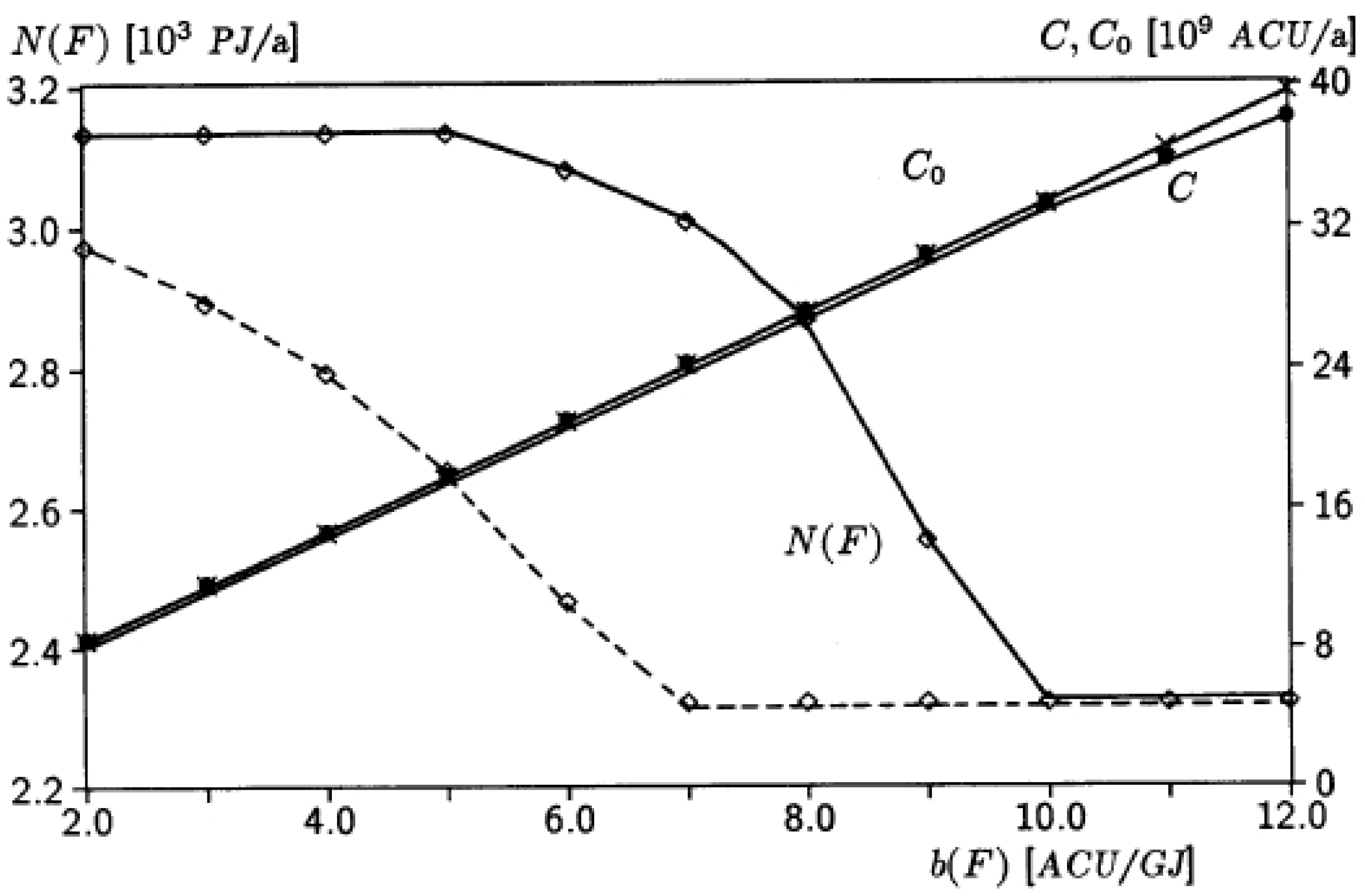
Figure 1 shows the result of energy optimization subject to upper cost limits for (west) Germany [37]. For the sake of simplicity, only one type of primary energy, called fuel F, has been considered. $N\left(F\right)$ is the number of units of fuel that are anually required to meet the fixed demand for energy services, as it is represented by the enthalpy-exergy demand profile. The associated annual cost, which is C with energy-conservation devices and $C_0$ without, includes costs of investment, maintenance, and fuel. The optimized annual demand for primary energy, $N\left(F\right)$, begins to decrease, when, at increasing fuel cost $b\left(F\right)$, total cost C can be reduced by reducing energy consumption via energy conservation.

If the upper cost limit $C_0$ must not be exceeded, $N\left(F\right)$ reaches its minimum at $b\left(F\right)=$ 10 ACU/GJ in Figure 1 [38]. (If 10-percent subsidies are possible, so that the upper cost limit is $1.1C_0$, the fuel-price increase that is necessary to exhaust the savings potential stops at 7 ACU/GJ.) For more details, like the specific costs of fuel burners and of the energy-conservation devices that partly replace them, annuities, and energy transportation distances, see [37].

Let us assume that in the idealized world of energy conservation, represented by the solid curve in Figure 1, there is an enlightened society in which the political leaders, public opinion, and the common man all agree that maximum energy conservation is the thing that should be done first to fight pollution, and that one should begin with the optimization scheme of Figure 1. In order to stimulate such a transformation of the energy system, the fuel price is quintupled by energy taxation [1,39] from $b\left(F\right)$= 2 ACU/GJ to $b\left(F\right)=$ 10 ACU/GJ at $t=t_C$ [40]. Then, the amount of primary energy required to satisfy the fixed demand for energy services will be reduced from its maximum at $N\left(F\right)\approx 3.15\times {10}^3$ PJ per year, at a total system cost of $C=C_{min}\approx 8\times {10}^9$ ACU per year, to its minimum at $N\left(F\right)=2.3\times {10}^3$ PJ per year, with the total system cost at $C_{up}\approx 33\times {10}^9$ ACU per year.

Thus, the full annual additional cost of capital, labor, and energy required for providing unchanged energy services at maximum energy conservation via heat exchanger networks (ex), heat pumps (hp) and cogeneration (cog) is

$$\Delta C_{ex,hp,cog}^f\equiv C_{up}-C_{min}=25\times {10}^9\mathrm{ACU}/\mathrm{year}\approx 25\times {10}^9{\$}_{1986}/\mathrm{year}.$$

(26)

An energy tax that, as assumed, quintuples the fuel price generates substantial revenues for the state treasury [41,42,43]. It may benefit society as a whole, if it is used to finance the systems of social security so that the taxes and levies on labor may be reduced signficantly. However, there are people who are afraid that tax increases whatsoever are venom for the economy and strangulate economic growth. They would reason that the loss of conventional output in our fuel-taxation and energy-conservation scenario [44] is given by the cost difference in Equation (26), and that it will have consequences for later times, too. Then, in this pessimistic view, the conventional output at $t=t_C$ would be

$$Y_C\left(K,L,E;t_C\right)=Y\left(K,L,E;t_C\right)-\Delta C_{ex,hp,cog}^f.$$

(27)

Inserting $Y_C(K,L,E;t_C)$ from Equation (24) and $Y\left(K,L,E;t_C\right)$ from Equation (25) into Equation (27), dividing by $Y(K,L,E;t_C)$, using [45] $Y_0\left(t_C\right)\cong Y_{C0}\left(t_C\right)$, and taking the logarithm yields the equation for the (output-elasticities-reducing) constant ${\varphi }_{\left\{p_i\right\}}$ as

$${\mathsf{\varphi }}_{\left\{p_i\right\}}=1+\frac{ln\left(1-\frac{\Delta C_{ex,hp,cog}^f}{Y_0\left(t_C\right)expF{(K,L,E)}_{t_C}}\right)}{F{(K,L,E)}_{t_C}}\equiv {\mathsf{\varphi }}_{\left\{p_i\right\}}^{\left(f\right)}.$$

(28)

Its numerical value $<1$ follows from $F{(K,L,E)}_{t_C}$, computed according to Equation (15) for known $\mathsf{\alpha },\mathsf{\beta },\mathsf{\gamma }$ at $K\left(t_C\right),L\left(t_C\right),E\left(t_C\right)$, and Equation (26).

The annuity method distributes the cost of the energy-conversion technologies to a number of years $t\ge t_C$. On the other hand, the system has become more energy efficient. An admittedly crude model assumption is that interest rates, maintenance costs, fuel price increase, and annuities can be chosen in such a way that the difference between the gains from energy conservation and the annual losses $\Delta C_{ex,hp,cog}^f$ are such that one obtains conventional output for times $t>t_C$ (wthin the time span restricted by the annuity method) by replacing $t_C$ in Equation (24) with $t\ge t_C$. Thus, the production function for conventional output, when pollution abatement is practiced via energy conservation stimulated by energy taxation, is

$$Y_C(K,L,E;t\ge t_C)=Y_0\left(t\right)exp\left\{{\mathsf{\varphi }}_{\left\{p_i\right\}}^{\left(f\right)}F{(K,L,E)}_{t\ge t_C}\right\},$$

(29)

with the number ${\mathsf{\varphi }}_{\left\{p_i\right\}}^{\left(f\right)}$ given by Equation (28).

Just to give an idea of how one might actually compute this number, we assume that $t_C$ is the year 1986 and that the annual cost $\Delta C_{ex,hp,cog}^f=25\times {10}^9{\$}_{1986}$ in Equation (26) would have been imposed on the (west) German sector “Industries” by triggering energy conservation via energy taxation as described above. (In reality, this did not happen. Rather, the substantial German worries about the forest-killing emissions of SO${}_2$ and NO${}_X$ led to legislation in the mid-1980s that very successfully enforced desulphurization and denitrification of the flue gases of power stations, and the catalytic converter for cars as well.)

The empirical output of the sector “Industries” of the Federal Republic of Germany in 1986 was about $880\times {10}^9{\mathrm{DM}}_{1991}$, see [1], p. 264. This corresponds to $440\times {10}^9{\$}_{1986}$, if, in a rough approximation, one assumes that $1{\$}_{1986}\approx {2\mathrm{DM}}_{1991}$. This output is well reproduced by the LinEx function $Y_{L1}(K_{1986},L_{1986},E_{1986};1986)$ [10], and we use its number for $Y_0\left(1986\right)expF{(K,L,E)}_{t_C=1986}$ in Equation (28). Thus,

$$\frac{\Delta C_{ex,hp,cog}^f}{Y_{L1}(K_{1986},L_{1986},E_{1986};1986)}=\frac{25\times {10}^9{\$}_{1986}}{440\times {10}^9{\$}_{1986}}\approx 0.06$$

(30)

is the relative reduction of conventional output. Furthermore, observing Equations (15)–(18), $F{(K,L,E)}_{t_C=1986}$ in Equation (28) is obtained by computing the logarithm $ln[Y_{L1}(K_{1986},L_{1986},E_{1986};1986)/Y_0\left(1986\right)]$. Although the technology constants a and c have somewhat varied in response to the oil-price shocks 1973–1981, we approximate $Y_0\left(1986\right)$ by the output of the German Sector “Industries” in the base year 1960. This output is $Y_0\left(1960\right)=453.5\times {10}^9$DM${}_{1991}\approx 227\times {10}^9{\$}_{1968}$, according to [1], p. 264. Then $F{(K,L,E)}_{t_C=1986}\equiv ln[Y_{L1}(K_{1986},L_{1986},E_{1986};1986)/Y_0\left(1986\right)]=0.66$. With this and Equation (30), one gets

$${\mathsf{\varphi }}_{\left\{p_i\right\}}^{\left(f\right)}=1+\frac{ln(1-0.06)}{0.66}=0.91$$

(31)

as the multiplier of the output elasticities. Thus, the reduction of output elasticities in the first, pessimistic scenario, which charges the full cost increase to energy conservation, is nearly 10%.

A second, more optimistic scenario for the same energy system is based on the trade-off between primary energy consumption and total cost at fixed fuel price $b\left(F\right)$. Figure 4 of [37] shows the trade-off curves that correspond to $b\left(F\right)$ = 4 ACU/GJ and $b\left(F\right)$ = 8 ACU/GJ. The trade-off curves are computed by optimizing a linearly weighted, two-component objective function, where the weights of the components “required fuel $N\left(F\right)$” and “cost C ” vary between 0 and 1. At $b\left(F\right)$= 4 ACU/GJ the quantity of fuel, $N\left(F\right)$, that is necessary to satisfy the fixed demand for energy services, reaches its minimum of $2.3\times {10}^3$PJ/year at a cost increase of 30%, or, in absolute numbers,

$$\Delta C_{ex,hp,cog}^0=5\times {10}^9\mathrm{ACU}/\mathrm{year}\approx 5\times {10}^9{\$}_{1986}/\mathrm{year}.$$

(32)

If, at the given fuel price $b\left(F\right)$ = 4 ACU/GJ, society decides to exhaust its energy conservation potential, and establishes rules that make all its members pay for it as in the pessimistic scenario, then $\Delta C_{ex,hp,cog}^0$ takes the place of $\Delta C_{ex,hp,cog}^f$ in Equations (30) and (28), and instead of Equation (30) and Equation (31) one has

$$\frac{\Delta C_{ex,hp,cog}^0}{Y_{L1}(K_{1986},L_{1986},E_{1986};1986)}=\frac{5\times {10}^9{\$}_{1986}}{440\times {10}^9{\$}_{1986}}\approx 0.012$$

(33)

and

$${\mathsf{\varphi }}_{\left\{p_i\right\}}^{\left(0\right)}=1+\frac{ln(1-0.012)}{0.66}=0.98.$$

(34)

Here, the reductions of conventional output and of the output elasticities are just 1% and 2%, respectively. The corresponding conventional output at times $t\ge t_C=1986$ is given by Equation (29), with ${\mathsf{\varphi }}_{\left\{p_i\right\}}^{\left(f\right)}$ being replaced by ${\mathsf{\varphi }}_{\left\{p_i\right\}}^{\left(0\right)}$.

3.2.3. Nuclear Exit, CO${}_2$ Abatement, and Photovoltaics Implementation

Valuation judgements, and uncertainties about the influence of present decisions on future developments, are crucial problems in economics. This does not only show in the two scenarios of energy conservation discussed above, but also in the question: “What are the appropriate energy carriers for the future?”

After the 2011 Fukushima catastrophe, when the tsunami that followed the 11 March earthquake destroyed insufficiently protected emergency generators of the Fukushima Daiichi power plants, causing the core meltdowns of three nuclear reactors and the explosion of a fourth one, Germans decided that nuclear power were too risky for them. The law of 2010, that had considerably extended the operation time of German nuclear reactors in order to reduce CO${}_2$ emissions, was revoked, eight nuclear power plants were shut down right away, and the last of the remaining nine ones is sheduled to cease operation in 2022. Since then, the majority of German citizens and politicians are convinced that renewable energies are the only acceptable non-fossil energies.

This is not the place to enter into the discussions of the precipitous German nuclear-exit decision and the chaotic energy policy thereafter. In the present article, the German priority for renewable energies only motivates considering scenarios of nuclear exit and aspired CO${}_2$-emission mitigation by the massive introduction of photovoltaics (PV) into the German energy system.

Before doing that, it is useful to have a look at the life-cycle CO${}_2$ emissions from important energy carriers and their energy-conversion technologies.

The estimates of the life-cycle CO${}_2$ emissions of photovoltaics in

Table 1. Specific total life–cycle CO${}_2$ emissions, in grams per kWh of electric energy, for different energy systems. Included are emissions from operation, maintenance, and production of the system. Emissions from waste disposal are excluded [46,47,48].

Energy System	Specific Total Life–cycle CO${}_2$ Emissions, g/kWh
Lignite-fired power plant	850–1200
Hard-coal-fired power plant	700–1000
Natural-gas-fired power plant	400–550
Photovoltaic cell	70–150
Gas-powered combined heat and power unit	≈ 50
Water power plant	10–40
Nuclear power plant	10–30
Wind park	10–20

take into account that by the year 2014 Chinese PV cells have conquered roughly two thirds of the world market, and of the German market as well, and that CO${}_2$ emissions of PV production are in China about twice as large as in Germany [46].

Table 2. Primary energy consumption in Germany [49].

Year	1991	1992	1999	2000	2010	2011	2012	2013	2014
${10}^{15}$ J	14,750	14,400	14,350	14,401	14,044	13,750	13,380	13,723	13,077

reports German primary energy consumption after reunification, and

Table 3. Shares of energy carriers in German primary energy consumption, in percent, rounded. Source: Arbeitsgemeinschaft Energiebilanzen.

Year	Mineral Oil	Natural Gas	Coal	Lignite	Nuclear Energy	Renewables
2010	33	22	12	11	11	9
2011	33	21	13	12	9	11
2013	33	22	13	12	8	11
2014	35	21	13	12	8	11

shows the shares of the principal energy carriers. The decrease in primary energy consumption between 1991 and 2012 is partly due to the shift of production from east Germany to the energetically more efficient west German factories, and to improved thermal housing insulation as well, and partly it is due to the long-term trend in many highly industrialized countries to outsource the production of energy-intensive goods to developing countries and concentrate on high-tech, high-priced goods and services instead.

Table 4. Shares of renewable energies in German electricity generation, in percent, rounded. Sources: Arbeitsgemeinschaft Energiebilanzen and Bundesverband der Energie- und Wasserwirtschaft.

Year	Total	Wind	Biomass	Water	Photovoltaics	Domestic Waste
2011	20	8	5	3	3	1
2013	23	8	7	3	5	n.a

indicates the shares of PV and other renewables in German electricity generation. Electricity generation requires roughly 16% of German primary energy. In 2014, renewables contributed about 28% to it. By then, the share of photovoltaics had increased to 1% in primary energy consumption and to roughly 6% in electricity generation (Source: Bundesumweltamt).

Specific CO${}_2$ emissions of gross electricity generation in Germany since 1991 are shown in

Table 5. Specific emissions of CO${}_2$ from German electricity generation, $I_1$, and consumption $I_2$ [50]. For the indicators $I_1$ and $I_2$ see the text.

Year	1991	2000	2007	2010	2011	2012	2013
$I_1$, g/kWh	744	627	602	542	558	562	559
$I_2$, g/kWh	745	623	623	559	564	586	595

. They include only the emissions from the direct combustion of fossil fuels. There are two indicators: $I_1$ gives the CO${}_2$ emissions in grams per kWh of electricity generated in Germany, and $I_2$ gives these emissions in grams per kWh of electricity consumed in Germany. Thus, if less electricity is consumed than generated in Germany, $I_2$ is larger than $I_1$. In 2014, Germany paid about 30 million Euros to neighboring countries for accepting surplus electricity from fluctuating wind power and photovoltaics. The surplus has to be accepted by the grid because of the legal obligations from the German Renewable Energy Law (GREL). Since 2011, the specific CO${}_2$ emissions in Table 5 no longer decrease. The increase of the specific CO${}_2$ emissions after 2010 is due to the substitution of lignite power plants for nuclear power plants. The specific life-cycle emissions from photovoltaics, Table 1, are not included in Table 5.

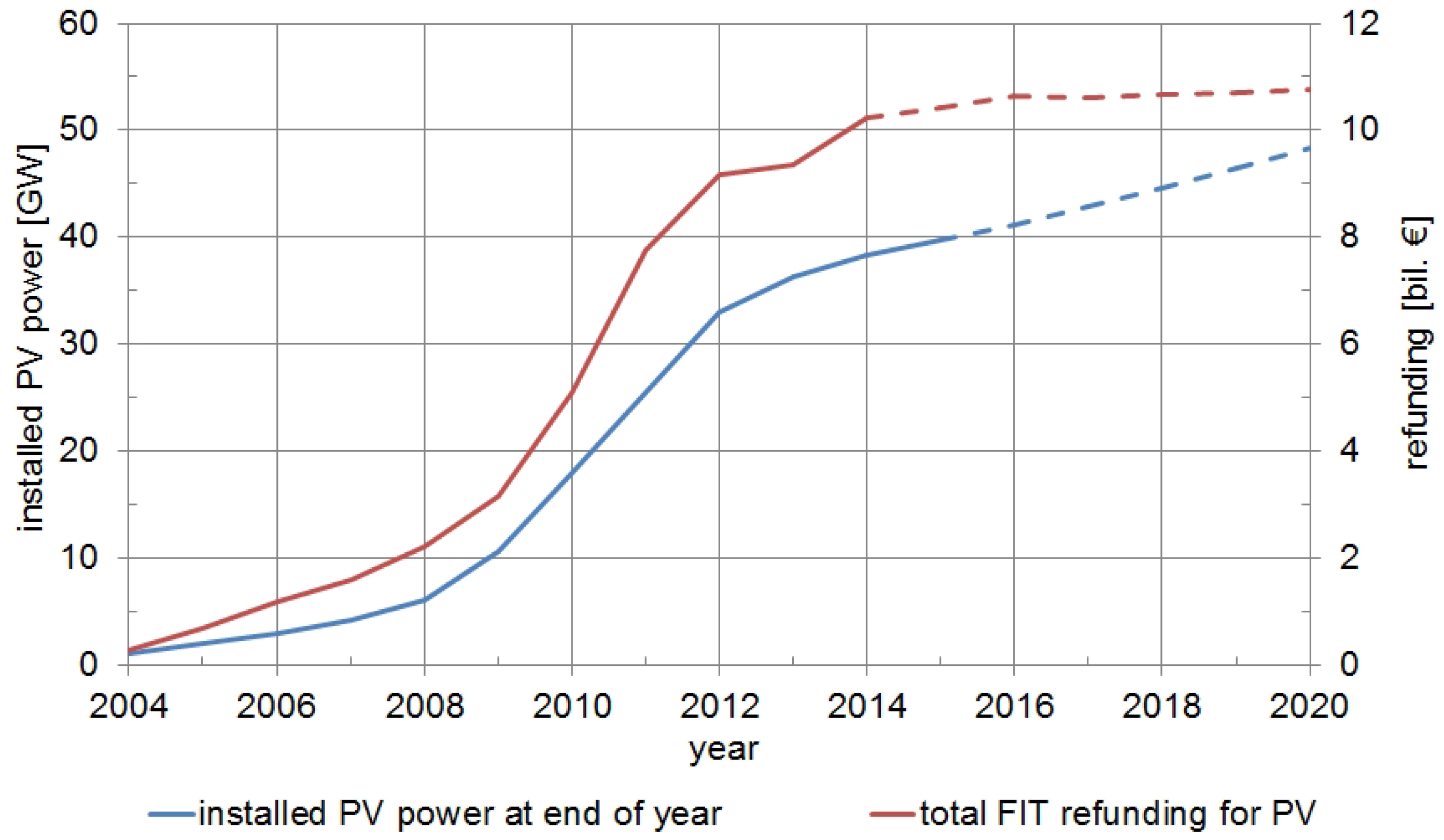
By the end of 2014, total German electricity-generation capacity was about 194 GW. Forty-five percent of that was renewables: 20% solar, 18% wind, whose capacities sum up to 74 GW, and 7% others. (Source: Bundesministerium für Wirtschaft und Energie, “Zahlen und Fakten”). Figure 2 shows the growth of the installed capacity of photovoltaic electricity generation and the annual payments (“refunding”) handed out to the PV-electricity producers according to the provisions of the (often reformed and rather complicated) German feed-in tariff (FIT) system, established by the GREL, which obliges (essentially private) consumers to subsidize the producers of renewable energies. It led to an average PV refunding of 32 ct/kWh in 2013 [51]; (ct = Eurocent) [52].

There have been lively debates on the cost of the renewables. Especially, people do not like the surcharge due to the GREL on their electricity bills, and many argue that industry should pay its share, too. There is no way of even trying to cut a clear path through the jungle of arguments on (i) hidden and open subsidies for fossil and nuclear fuels, on the one hand, and renewables, on the other hand, (ii) the external costs of energy carriers and their conversion technologies, including the problem of discounting future damages [1,53], and (iii) the comparison and valuation of risks. Rather, let us play with the above-mentioned numbers concerning specific CO${}_2$ emissions, Watts, Joules, and Euros in the two scenarios (A and B) that lead to the results in

Table 6. German gross domestic product (GDP) until 2014 and GDP${}_a$ afterwards, and refunding ${\Lambda }_{PV}$ of PV-electricity generation according to scenarios A and B, in billion Euros. ${\Lambda }_{PV}$-numbers of scenario A are from Figure 2 and the linear average of the upper curve after 2013, ${\Lambda }_{PV}$-numbers of scenario B are constructed by adding 2 billion Euros per year to the 2011 refunding in Figure 2. GDP is from Table 7, GDP${}_a$ is from Equation (35).

Year	2011	2012	2013	2014	2015	2016	2017	2018
GDP||GDP${}_a$	2670	2691	2698	2740	2765	2790	2815	2840
${\Lambda }_{PV}$,scenario A	8	9	9.5	9.7	9.9	10.1	10.3	10.5
${\Lambda }_{PV}$, scenario B	8	10	12	14	16	18	20	22

.

The refunding on the right ordinate of Figure 2, annually paid to the (mostly decentralized) providers of PV electricity by the consumers, correspondingly reduces the latter’s (debt-free) consumption of goods and services from the traditional basket [54]. It represents the loss in Equation (19), with ${\Lambda }_m\ne 0$ only for $m=PV$, and ${\Lambda }_{PV}=$ refunding.

In order to avoid runaway PV subsidies, a legal barrier of 52 GW on photovoltaics capacity has been introduced recently, despite strong opposition from PV lobbyists. Once it will have been reached, the annual payments to the providers of PV power are expected to not exceed 10–11 billion Euros [51]. Without that limitation, and assuming a linear extrapolation of the 2010 refunding gradient in Figure 2, the annual PV subsidies ${\Lambda }_{PV}$ would increase by roughly 2 billion Euros per year.

Let us consider two scenarios of PV implementation and the resulting reduction of conventional output. They begin with the year 2011 in Table 6. Scenario A is with the legal barrier on PV capacity, and Scenario B is without. The total German output is given by the GDP in

Table 7. German gross domestic product (GDP) after German reunification, inflation-corrected, chained, in billion Euros${}_{2010}$, rounded; and growth rates. Source: Statistisches Bundesamt [55].

Year	1991	1992	1999	2000	2010	2011	2012	2013	2014
GDP, ${10}^9$ Euros	2045	2076	2286	2358	2580	2670	2691	2698	2740
growth rate, %	n.a	1.5	1.9	3.2	3.9	3.7	0.6	0.4	1.6

. For the scenario years after 2014, numbers are used that result from the 2014 output and its growth with the average of the 2012–2014 growth rates, which is roughly 0.9%. Thus, the assumed GDP of the year 2014+n in Table 6 is

$${\mathrm{GDP}}_a={\mathrm{GDP}}_{2014}{(1+0.009)}^n.$$

(35)

Table 3, Table 4 and Table 5 show the success of German energy policy on emission mitigation after 11 March 2011. Right now, this policy does not support enthusiasm, even if one takes into account that after 2022, when the last German nuclear reactor will have ceased operation—and if German energy policy will not perform another U-turn—it will prevent further growth of nuclear waste, which emits ionizing particles and photons. It is a matter of risk-perception and -valuation, whether or not one considers the losses of conventional GDP in Table 6 as an acceptable PV share of the price for the still ongoing shake-up of the German energy system.

Thus, the relative loss of conventional GDP in 2014 would be about 0.4% in scenario A and 0.5% in scenario B. In 2018, the losses would be 0.4% and 0.8%. Of course, recessions would increase the percentages of the losses.

4. Summary and Outlook

Emissions from entropy production, which is coupled to energy conversion, are becoming a major problem for industrial economies. Abating them requires certain shares of capital, labor, and energy, which are missing for the production of convential output, i.e., the output that would be available to investors and consumers, if there were no need for pollution abatement. The impact of emission mitigation on economic growth is estimated by two methods. (1) The output elasticities of the production factors in the growth equation are multiplied by products of pollution functions and their technology multipliers. They model society’s response, when it becomes aware of critical limits to pollution and decides to reduce emissions. The model is applied to scenarios, whose empirical data are related to Germany before reunification. Two scenarios treat a fictitious case of energy conservation by thermoeconomic energy and cost optimization in (west) German industry. They yield losses of conventional output of about six and one percent of total output. Relative reductions of output elasticities are at 10 and two percent. The production function for coventional output is obtained from the known production function for total output. The latter, the measure of all economic activities, is listed in the national accounts as gross domestic product (GDP), or parts thereof. (2) The direct way of estimating the evolution of conventional output subject to emission mitigation is subtracting the resulting losses, i.e., the monetary values of goods and services dedicated to pollution abatement, from total output. This method is demonstrated for two scenarios of Germany’s nuclear exit and accelerated introduction of renewables after the Fukushima catastrophe. Data are available for the years from 2011 to 2018. The losses, just because of the subsidies to photovoltaics, are between 0.4 and 0.8 percent of GDP.

The methods proposed and the results obtained in this article are only a first step toward estimating the impact of entropy production on economic growth. Further research is required. It should be applied to countries in the process of actually fighting pollution. Of interest are scenarios, where the output elasticities of capital, labor, and energy for conventional output are reduced relative to those for total output by the same factor, as in this article, and by different factors as well. In the latter case, the production function for conventional output will depend on the path in factor space along which the “polluted” growth equation is integrated. The method of reduced output elasticities is based on production functions for total output, and the corresponding output elasticities. To compute them, one needs new, updated time-series of consistent sets of reliable empirical data on total output, capital, labor, and energy. Construction of such data base requires time and money [56]. The alternative method of calculating the evolution of conventional output from time series of total output and of expenditures for emission mitigation requires profound engineering and business knowledge concerning mitigation technologies.

References and Notes

- Kümmel, R. The Second Law of Economics—Energy, Entropy, and the Origins of Wealth; Springer: New York, NY, USA; Dordrecht, The Nertherlands; Heidelberg, Germany; London, UK, 2011. [Google Scholar]
- Microscopic descriptions are by Green’s functions and density functional theory in physics and by game theory in studies of economic behavior.
- Proops, J.L.R. Thermodynamics and Economics: From Analogy to Physical Functioning. In Energy and Time in the Economic and Physical Sciences; van Gool, W., Bruggink, J.J.C., Eds.; North-Holland: Amsterdam, The Nertherlands; New York, NY, USA; Oxford, UK, 1985; pp. 155–174. [Google Scholar]
- Richmond, P.; Mimkes, J.; Hutzler, S. Econophysics and Physical Economics; Oxford University Press: Oxford, UK, 2013. [Google Scholar]
- The experimental knowledge required to calculate S is (1) the heat capacity as a function of absolute temperature T for some one fixed value V1 of the system volume V; and (2) the equation of state of the system [6], p. 171f.
- Reif, F. Fundamentals of Statistical and Thermal Physics; McGraw-Hill: New York, NY, USA, 1965. [Google Scholar]
- Barbaresco, F. Koszul Information Geometry and Souriau Geometric Temperature/Capacity of Lie Group Thermodynamics. Entropy 2014, 16, 4521–4565. [Google Scholar] [CrossRef]
- Although the production function is a widely accepted tool of standard econometrics, it has been severely criticized by economists who are concerned about aggregation and physical aspects of production; see, e.g., the references [88–93] in Chapter 4 of [1]. The response to this criticism, which justifies the twice-differentiable production function, precisely by aggregating output and factors in terms of work performance and information processing, is on pp. 252–260 of [1].
- If technological constraints on factor combinations are taken into account in the optimization of profit or time-integrated utility, the resulting equilibrium is far from that of neoclassical economics, and the profit function ceases to be the Legendre transform of the production function [1,10].
- Kümmel, R.; Lindenberger, D. How energy conversion drives economic growth far from the equilibrium of neoclassical economics. New J. Phys. 2014, 16, 125008. [Google Scholar] [CrossRef] For a summary of the KLEC model and the implications of its findings for energy policy, and further literature on energy in the modeling of economic growth, see also Kümmel, R.; Lindenberger, D.; Weiser, F. The economic power of energy and the need to integrate it with energy policy. Energy Policy 2015, 86, 833–843. [Google Scholar]
- Implicitly, the Second Law is behind all talk about “energy consumption”, which really means exergy destruction.
- Georgescu-Roegen, N. The Entropy Law and the Economic Process; Harvard University Press: Cambridge, MA, USA, 1971. [Google Scholar]
- Letters to the Editor. Recycling of Matter. Ecol. Econ. 1994, 9, 191–196.
- Prigogine, I.; Nicolis, G. Biological order, structure and instabilities. Q. Rev. Biophys. 1971, 4, 107–147. [Google Scholar] [CrossRef] [PubMed]
- Prigogine, I.; Nicolis, G.; Babloyantz, A. Thermodynamics of evolution. Phys. Today 1972, 25, 23–28. [Google Scholar] [CrossRef]
- Thus, total entropy balance dS/dt is positive and entropy increases in V, if less entropy is transported out of V by JS than is being produced in V by σS; otherwise, dS/dt is negative or vanishes.
- Its equivalent technical formulation says that one cannot build a Perpetuum Mobile of the Second Kind.
- Kammer, H.-W.; Schwabe, K. Thermodynamik Irreversibler Prozesse; Physik-Verlag: Weinheim, Germany, 1986; p. 60. [Google Scholar]
- Fricke, J.; Borst, W. L. Energie, 2nd ed.; Oldenbourg: München, Wien, 1984; p. 40ff. [Google Scholar]
- Kluge, G.; Neugebauer, G. Grundlagen der Thermodynamik; Spektrum Fachverlag: Heidelberg, Germany, 1993. [Google Scholar]
- The conductive current densities jQ and jk are the respective current densities minus the center-of-mass velocity v(r, t) multiplied by the appropriate densities of internal energy and mass.
- Pollutants from energy carriers, their sources, and their noxious effects are listed on p. 136 of [1].
- “Emission mitigation” and “pollution abatement” are used synonymously.
- Potential energy stored in buildings is relatively small and turns into heat once the buildings are torn down. Similarly, oxidation of chemical products releases stored chemical energy as heat.
- International Energy Agency. Key World Energy Statistics 2015. Available online: http://www.iea.org/publications/freepublications/publication/KeyWorld_Statistics_2015.pdf (accessed on 9 February 2016).
- Von Buttlar, H. Umweltprobleme. Phys. Blätter 1975, 31, 145–155. [Google Scholar] [CrossRef]
- Berg, M.; Hartley, B.; Richters, O. A stock-flow consistent input-output model with applications to energy price shocks, interest rates, and heat emissions. New J. Phys. 2015, 17, 015011. [Google Scholar] [CrossRef]
- The time tCi is not only determined by the physical, chemical, and biological consequences of pollution, but also by economic and social factors like standard of living and the set of values important to society.
- Ayres, R.U.; Warr, B. Accounting for growth: Role of physical work. Struct. Change Econ. Dynam. 2005, 16, 181–209. [Google Scholar] [CrossRef]
- Ayres, R.U.; Warr, B. The Economic Growth Engine; Edgar Elgar: Cheltenham, UK, 2009. [Google Scholar]
- The basic physical aggregation of output and capital in terms of work performance and information processing, and its relation to constant currency, is elaborated in Appendix 3 to Chapter 4 of [1].
- Kamke, E. Differentialgleichungen II; Akademische Verlagsgesellschaft: Leipzig, Germany, 1962; pp. 1–27. (In German) [Google Scholar]
- Standard economics uses Cobb-Douglas functions with the variables K and L frequently, those with K, L, and E occasionally.
- External Environmental Costs of Electric Power; Hohmeyer, O.; Ottinger, R.L. (Eds.) Springer: Berlin/Heidelberg, Germany, 1991.
- Stern, N. The Economics of Climate Change. Amer. Econ. Rev. 2008, 98, 1–37. [Google Scholar] [CrossRef]
- Then, Equation (20) is an ad-hoc equation in the sense that it does not result from a state function’s total differential, whereas Equation (7) does.
- Groscurth, H.-M.; Kümmel, R. The cost of energy optimization: A thermoeconomic analysis of national energy systems. Energy 1989, 14, 685–696. [Google Scholar] [CrossRef]
- ACU/GJ= Arbitrary Currency Unit per Giga Joule. A primary energy price of 4 ACU/GJ approximately corresponds to 24 US$ per barrel oil in 1986. Thus, with GJ/barrel = 0.18, 1 ACU≈ 1$1986.
- For example, by shifting the burden of taxes and levies from labor to energy, as discussed in [1], p. 278ff.
- Such a fuel-price hike would somewhat exceed the oil-price explosion between 1973 and 1975.
- Hannon et al. discuss energy conservation taxes [42], and Baron analyzes competitive issues related to carbon/energy taxation [43].
- Hannon, B.; Herendeen, R.A.; Penner, P. An energy conservation tax: Impacts and policy implications. Energy Syst. Policy 1981, 5, 141–166. [Google Scholar]
- Baron, R. Competitive issues related to carbon/energy taxation. In Annex I Expert Group on the UN FCCC, Working Paper 14; ECON-Energy: Paris, France, 1997. [Google Scholar]
- This is Λm in Equation (19) at t = tC with only one term m ≡ ex, hp, cog.
- The integration constants Y0, YC0 are free parameters, which, together with a and c in the case of the LinEx function (18), are determined by SSE minimization. In the approximations of this subsection, the pollution functions affect the output elasticities as a whole, but not the free parameters individually.
- Stoller, D. Chinesische Solarzellen haben eine verheerende Umweltbilanz. Available online: http://www.ingenieur.de/Themen/Photovoltaik/Chinesische-Solarzellen-verheerende-Umweltbilanz (accessed on 15 August 2015).
- Wagner, H.-J.; Koch, M.K. CO2-Emissionen der Stromerzeugung. BWK 2007, 59, 44–52. [Google Scholar]
- Mauch, W. Kumulierter Energieaufwand—Instrument für nachhaltige Energieversorgung. Forschungsstelle für Energiewirtschaft Schriftenreihe 1999, 23, 65–76. [Google Scholar] Combined with data from Öko-Institut Darmstadt 2006.
- Arbeitsgemeinschaft Energiebilanzen e.V. Available online: http://www.ag-energiebilanzen.de (accessed 20 August 2015).
- Icha, P. Entwicklung der spezifischen Kohlendioxid-Emissionen des deutschen Strommix in den Jahren 1990 bis 2013. Umweltbundesamt: Dessau-Rosslau, Germany, 2015; 12. [Google Scholar]
- Wirth, H. Aktuelle Fragen zur Photovoltaik in Deutschland; Fassung vom 19.5.2015; Fraunhofer-Institut für Solare Energiesysteme ISE: Freiburg, Germany; Available online: http://www.pv-fakten.de (accessed on 27 August 2015).
- My 2015 electricity bill charged 21 ct/kWh, which included 6.2 ct/kWh due to the GREL; in 2010 the numbers were 21 ct/kWh and 3.6 ct/kWh.
- see, e.g., pp. 242 ff of [1].
- Fossil and nuclear fuels could satisfy all demand for electricity in Germany. But the decision to perform the nuclear exit in conjunction with CO2 abatement requires the massive introduction of renewables, with much emphasis on photovoltaics. One might also reason that the precipitous nuclear exit after 11 March 2011, should be considered as an additional reduction of conventional output, this time of its investment component. However, a German energy economist, who frequently appears on television, first hailed the 2010 law that extended the operation time of German nuclear power plants, which had been continuously refitted to meet increasing safety standards, as an economically sound use of prior investments. Nevertheless, when the mood changed after the Fukushima catastrophe, she became a strong supporter of the U-turn in German energy policy. Given such drastic changes in the economic valuations of the substitution of renewables for nuclear energy, the reduction of conventional output by sunk costs and new investments is too uncertain a matter to be considered here.
- Statistisches Bundesamt. Available online: http://www.destatis.de (accessed on 7 September 2015).
- When I entered econometrics in the 1980s, experts in the field advised me not to use easily availabe, but unreliable data from secondary sources, but to go to the original sources always. These are the national accounts for inflation-corrected output and capital, the national labor statistics, and the national energy balances. Chaining different time-series sections was not a minor problem for US data, and the Japanese data sources could only be evaluated with the kind help of colleagues from Japanese energy reseach instututions. Recently, German time series from 1960-2010 have been constructed in the Cologne Institute of Energy Economics. Ongoing research is based on them.
Figure 1.
Optimized potentials of energy conservation by heat-exanger networks, heat pumps, and cogeneration in the Federal Republic of Germany as a function of the price of one unit of fuel F [37]. is the annual quantity of primary energy required to satisfy the fixed demand for process heat and electricity. C and are the total annual costs of providing with and without energy-saving technologies. Solid curve: upper cost limit is ; dashed curve: upper limit is . Note the suppressed zero point of the ordinate. The figure is reproduced with kind permission of H.-M. Groscurth.
Figure 2.
Growth of installed PV capacity (lower curve, left ordinate, GW) and of annual PV refunding (upper curve, right ordinate, billion Euros) in Germany. This figure is reproduced with kind permission of H. Wirth. It is part of a forthcoming English version of [51]. Solid curves: actual data, dashed curves: projections.