Assessing the Robustness of Thermoeconomic Diagnosis of Fouled Evaporators: Sensitivity Analysis of the Exergetic Performance of Direct Expansion Coils

Abstract

Thermoeconomic diagnosis of refrigeration systems is a pioneering approach to the diagnosis of malfunctions, which has been recently proven to achieve good performances for the detection of specific faults. Being an exergy-based diagnostic technique, its performance is influenced by the trends of exergy functions in the “design” and “abnormal” conditions. In this paper the sensitivity of performance of thermoeconomic diagnosis in detecting a fouled direct expansion coil and quantifying the additional consumption it induces is investigated; this fault is critical due to the simultaneous air cooling and dehumidification occurring in the coil, that induce variations in both the chemical and thermal fractions of air exergy. The examined parameters are the temperature and humidity of inlet air, the humidity of reference state and the sensible/latent heat ratio (varied by considering different coil depths). The exergy analysis reveals that due to the more intense dehumidification occurring in presence of fouling, the exergy efficiency of the evaporator coil eventually increases. Once the diagnostic technique is based only on the thermal fraction of air exergy, the results suggest that the performance of the technique increases when inlet air has a lower absolute humidity, as evident from the “optimal performance” regions identified on a psychrometric chart.

1. Introduction

In the last decades great efforts have been made to improve the efficiency of air-conditioning units, as proven by the growth of Certification Programmes [1], both in terms of coverage among manufacturers and refinements in standard ratings, and by the wide research activities concerning the new refrigerants [2] and the technological solutions for enhanced heat transfer [3].

Unfortunately, despite this great effort in developing components and systems with higher nominal efficiency, less attention has been paid to the problem of improper/insufficient system maintenance. Extensive surveys have revealed that refrigeration units integrated in air conditioning systems are often poorly maintained and experience dramatic degradation of performance due to the presence of malfunctions or “faults” [4]. Among the most commonly detected faults, despite all electrical failures, the authors identified the frequent presence of dirty coils, refrigerant leakages from the high to the low pressure side of the compressor and refrigerant leakages to the ambient eventually resulting in undercharge. Efficient troubleshooting is not sufficient, since repairs are often invoked when the system is already experiencing the presence of “heavy faults” that eventually lead it out-of-service; conversely, the attention should be more and more focused on the detection of “soft faults”, that do not cause the unit stop functioning, but only induce degradation in plant performance provoking a decrease in the cooling capacity and a reduction in the Coefficient Of Performance (COP).

Actually, the the has been already addressed in literature. The scientific community has been developing more and more refined Faults Detection and Diagnosis (FDD) techniques, oriented to identifying faults affecting plant performance, thus allowing for maintenance aimed at restoring efficient operating conditions. Earlier studies were oriented to develop a “symptom matrix”, where for each fault the expected changes of different thermodynamic parameters were qualitatively recorded, in terms of either increase (↑) or decrease (↓) [5]. More recent works, however, have proposed new model-based FDD techniques for systems not heavily instrumented; in general, the diagnostic capability resulted from the evaluation of “residuals”, i.e., differences between the measured values of some thermodynamic parameters and their “expected values” [6].

The aforementioned diagnostic approaches suffer the possible presence of multiple faults, which is a quite common condition in refrigeration systems, especially for air conditioning applications. Then, an interesting approach has been proposed in [7], based on the use of “decoupling features”, i.e., thermodynamic variables (or their combinations) that are prevalently influenced by a unique fault and thus suitable for problem decomposition in multi-faults systems.

All the above described FDD techniques, however, share in common a limit that is essentially related with the qualitative nature of their results: even when a fault is correctly identified, the procedure does not allow one to assess whether we are in presence of a “light” or a “heavy” fault nor, in case of multiple simultaneous faults, to quantify the degradation of plant performance induced by any individual fault.

Then, a growing interest has been emerging for possible applications of thermoeconomic diagnosis, due to its intrinsically quantitative nature; thermoeconomic diagnosis is aimed at detecting efficiency deviations and evaluating their economic worth to identify the main causes that originated the performance degradation. The “fuel impact approach”, in particular, assumes a “productive structure” of the energy system (a representation alternative to its physical lay-out) where the interactions between components are identified basing on their functional relation. The resources consumed by each component (namely, its “fuels” F) and its useful outputs (namely, its “products” P) are preliminarily evaluated in exergy terms; then, a peculiar syntax based on cost balances and appropriate cost allocation rules [8] allows the analyst to disaggregate the additional fuel consumption into contributes associated with the malfunctions occurring in each component. Thermoeconomic diagnosis has been rarely applied to refrigeration systems for several reasons:

-

The application of thermoeconomic diagnosis to vapour compression cycles is quite difficult and the reliability of results hasn’t been proven yet. The performance of any plant component, in fact, is heavily influenced by all other components (due to system balancing); then, the effects of any fault will propagate to the whole plant, according to quite complex relationships. This problem has been addressed in literature [9,10], decomposing the additional exergy destructions observed at component level (due to local decrease of exergy efficiency) into “intrinsic malfunctions”, directly provoked by anomalies on the component, and “induced malfunctions”, i.e., malfunctions induced by changes in the operating point of the component (eventually provoked by intervention of the control system) [11] and consequent variations in its efficiency;

-

Difficulties are encountered when developing the “productive structure”, which requires any component to be modelled as a consumer of a fuel “F” and producer of a product “P”. The conceptual ambiguities are mainly related with the “condenser” and the “throttling valve”. The former represents a “dissipative component”, i.e., a device whose productive purpose (to discharge heat allowing to close the thermodynamic cycle of refrigerant) can be hardly expressed as a useful exergetic product. Several approaches have been proposed in literature, allocating the cost of the “residues” generated on the different components proportionally to their “negentropy” consumption [12,13] or to the exergy of the flows processed in the dissipative units according to the productive structure of the plant [14]. As concerns the expansion valve, the conventional thermoeconomic approach assumes this component to represent a productive unit, which consumes “mechanical exergy” to produce an increase of refrigerant “thermal exergy” [15]; however, this approach has been proven controversial [16].

A first example of comprehensive thermoeconomic diagnosis of refrigeration plants has been presented in [13], adopting the “fuel impact” approach. However, in this paper lacks controversial arguments, since the diagnosis is performed for a generic off-design state, not providing details about the set of faults that led to the abnormal operating condition.

In a recent paper by Piacentino and Talamo [17] some innovative solutions have been proposed, consisting of an original approach to model the dissipative components (the expansion valve and the condenser) and on an improvement in the diagnostic performance achievable by preliminarily filtering the effects of “system level” faults like refrigerant undercharge. The proposed approach has been tested for several combinations of multiple faults, in case of light and heavy performance (i.e., COP) degradation, achieving very promising results both in qualitative (capability of the technique to identify the faulty components) and quantitative (estimation of the increased energy consumption induced by each fault) terms. Analysing in details the methodological fundamentals of the improved thermoeconomic approach adopted in [17] is beyond the scope of the present paper.

Being this diagnostic method based on exergy flows, however, it’s worthwhile verifying whether (and at what extent) its performance is sensitive to boundary conditions; in fact, the very good performance achieved in the referenced paper was obtained for a specific operating condition, and it is evident that the exergy values may experience very high fluctuations when changing some thermodynamic parameters of the operating fluids. From this perspective the evaporator is probably the most critical component, due to the contemporary air cooling and dehumidification processes occurring across it, that induce significant variations in both the chemical and thermal fractions of air exergy. For this reason, the aim of this work is to investigate the sensitivity of the performance of the diagnostic technique proposed in [17] to the parameters that mostly influence the exergetic performance of the evaporator, assuming different operating conditions in terms of:

-

temperature and relative humidity of the air entering the direct expansion (DX) coil;

-

coil depth (modified by assuming different number of rows), since this parameter influences the dehumidification capacity of the coil and the sensible/latent heat ratio.

2. Methodology

The analysis was carried out through a number of consecutive steps, listed below:

• Definition of the reference plant scheme and of a number of scenarios, developed so as to put into evidence the sensitivity of performance of the diagnostic technique to the examined design variables and boundary conditions;
• Simulation of plant performance for all the examined scenarios, both in case of presence and absence of the examined fault (i.e., in presence of clean and fouled/dirty evaporator coil);
• Evaluation of all the exergy flows associated with the refrigerant and air flows;
• Implementation of the thermoeconomic diagnosis, based on the innovative technique proposed in [17];
• Sensitivity analysis of the performance of the thermoeconomic diagnostic technique for the examined scenarios, and interpretation of results.

The different steps will be described in separate sections below in the paper. While some aspects will be discussed in brief, having been accurately presented in previous referenced works, step 5 in the above list will be discussed in much more detail, since the insights emerging from the sensitivity analysis represent the main innovative contribution of this paper to the state of art on thermoeconomic diagnosis of air conditioning units.

3. Definition of the Reference Scheme and of the Examined Scenarios

The plant consists of a 120 kW air-cooled air conditioning rooftop unit that includes:

-

Two Copeland D4SA-200X reciprocating compressors (322 cm³ displacement each).

-

A finned condenser with 15.9 mm tube diameter, 14 fins per inch spacing and a compactness ratio of 913.8 m²/m³.

-

A thermal expansion valve (TXV) that imposes a fixed 6 °C superheating at the evaporator outlet.

As concerns the design of the evaporator, a fixed 1.92 m² face area was assumed (resulting from the 2400 × 800 mm size), while in the present paper three different coil depth were examined, characterized by a fixed 25 mm transversal spacing between consecutive rows. All the geometrical details of the main components and piping (i.e., discharge, liquid and suction lines) have been provided in [18]; the refrigerant is R407C. The reader is referred to the cited article for a detailed description of all the geometrical specifications of the plant.

As concerns the examined scenarios, an ambient temperature T₀ = 307.15 K (t₀ = 34 °C) was assumed, while different values of ambient relative humidities ϕ₀ (40%, 70% and 100%) were selected. In order to perform simulations, different conditions were assumed:

-

Five different air inlet temperatures at the evaporator coils, equal to 22 °C, 25 °C, 28 °C, 31 °C and 34 °C. While the former three values (22, 25 and 28 °C) may be conceived as more or less realistic set-point conditions for indoor comfort (depending on the clothing level and internal activity performed in the cooled ambient), the last two values (31 and 34 °C) represent possible inlet temperatures in case that the remote cooling units threats only “external air” or that a very low air recirculation rate is considered;

-

Three different air inlet relative humidities, equal to 45%, 60% and 75%;

-

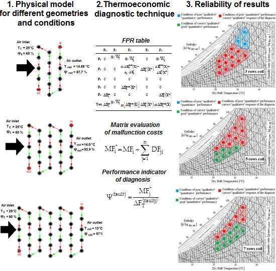
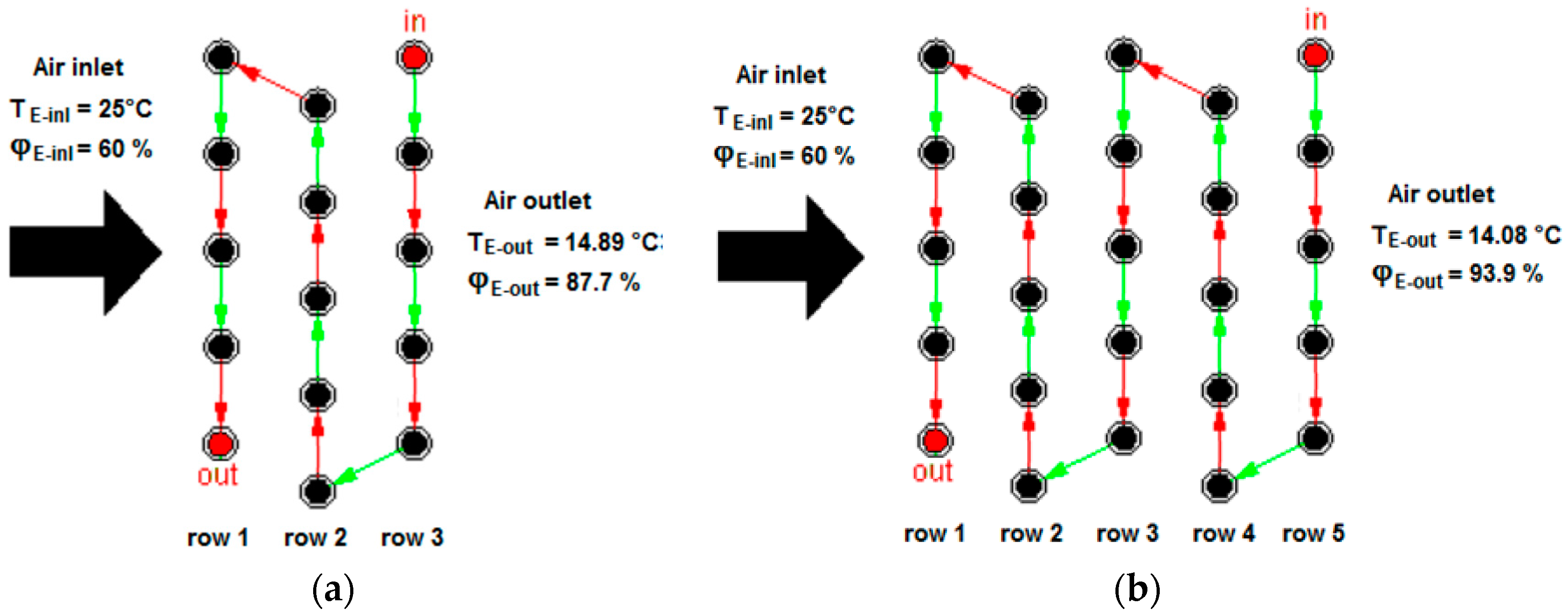
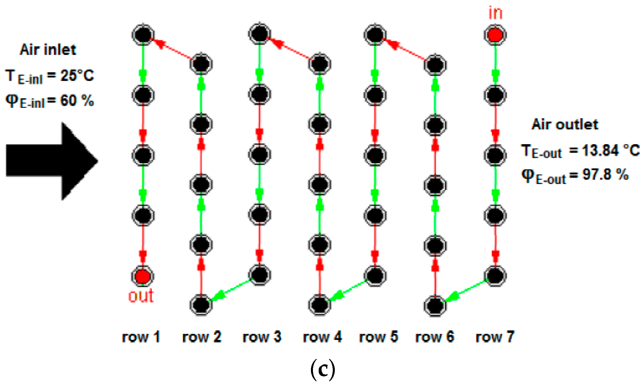
Three different coil depths, respectively equal to 3, 5 and 7 rows [19]. The scope for examining these three different geometries is evident in Figure 1, where the results obtained for the particular air inlet conditions T_E-inlet = 25 °C and ϕ_E-inlet = 60% are presented for the clean coils; from an analysis of Figure 1 we may observe that the dehumidification capacity increases with coil depth, as testified by the increasing relative humidity of the cold air exiting the coil. This is obviously due to the reduction of the by-pass factor of coils when the number of rows increases;

-

Two general operating conditions, related with the presence or the absence of the evaporator fouling (i.e., dirty or clean coil).

Therefore, the total number of plant simulations performed is 5 × 3 × 3 × 2 = 90 (referring to 45 combinations of inlet air conditions and coil geometries and two operating conditions, i.e., “dirty coil” and “design”).

As any thermoeconomic model requires the material streams and the components to be easily identified, the main plant components and the material streams were numbered consecutively, respectively by Arabic numerals (from 1 to 4) and by letters (from A to D for the refrigerant and by E and G for air), according to the simple notation presented in Figure 2. No “line faults” were considered in this study, and then the thermodynamic state of the refrigerant exiting a component were assimilated with that of the fluid entering the successive one (i.e., A ≡ A', B ≡ B', C ≡ C', D ≡ D').

4. Plant Simulations of the Examined Scenarios

The simulations were performed using the tool IMST-ART Version 3.60 [20], that implements the Finite Volume Method (FVM) to produce a discretization of coils’ surface and simulate the heat and mass transfer processes. Performance maps of the compressor and the fans were also adopted. The tool has been proven highly reliable, basing on comparisons with experimental data [21].

The tool does not include specific options to simulate a fouled evaporator; however, it allows for introducing “an enhancement factor” of pressure drops through the coil on the air-side, that is the largely prevalent effect of fouling on coils (since it implies a significant reduction in the air-velocity across the coil). In Ref. [19], in fact, it has been shown that while a heavy fouling induces increases in the air-side pressure drop in the order of 30%–50% compared to the clean coil (for a given air velocity), the induced change in the heat transfer coefficient is much lower (reduction in the order of 3%–5% is observed, for a given air velocity). IMST-ART implements a detailed heat exchangers model that determines heat transfer coefficients by built-in correlations and solves heat and mass transfer equations by FVM, discretizing the surfaces into a series of one dimensional paths of 1D-cells. Then, in order to simulate the effects of the examined fault, appropriate adjustments were made to the “pressure drop enhancement factor”, so as to simulate clean coils (corresponding to average air face velocity w_air equal to 2.7 m/s) and dirty/fouled coils (achieving a w_air = 2.1 m/s); the changes induced on the heat transfer coefficient due to the lower air velocity were determined by the routine.

The convenience of using thermodynamic data derived from plant simulations, rather than from experimental campaigns, is largely proven in the literature for such kind of problems. In fact, complex experimental campaigns would have been needed to acquire data on systems with clean and dirty coils, over such a wide range of possible operating conditions. Also, the use of a simulator is particularly appropriate for “what-if analyses” [8], since it yields flexibility in developing “faulty operation” scenarios, thus allowing for an efficient testing of the diagnosis technique; finally, in a recent work [22] the use of numerical-based diagnosis has been validated as an option to perform the diagnosis of a refrigeration system. Below in the paper all the thermodynamic parameters obtained by plant simulation had been preliminarily compared with experimental trends available in literature to ensure that they were realistic. In order to give a synthetic view of the effects induced by coil fouling, in

Table 1. Outlet air conditions for the clean and dirty coils, provided by the plant simulator for all the examined scenarios in case of a 5-rows coil depth.

Air Inlet Conditions		Air Outlet Conditions
		Clean Coil			Fouled Coil
T (°C)	ϕ (%)	T (°C)	ϕ (%)	Gair (kg/s)	T (°C)	ϕ (%)	Gair (kg/s)
22	45	9.5	91	7.14	7.0	93	5.77
22	60	11.4	94	6.90	9.8	96	5.53
22	75	13.4	96	6.82	12.0	97	5.55
25	45	11.8	91	6.96	10.5	93	5.63
25	60	14.1	94	6.77	12.6	95	5.47
25	75	16.3	96	6.73	14.9	97	5.38
28	45	14.4	91	6.88	12.8	93	5.54
28	60	16.9	94	6.69	15.4	95	5.40
28	75	19.3	95	6.64	17.9	96	5.31
31	45	16.8	92	6.68	15.2	93	5.31
31	60	19.7	94	6.53	18.2	95	5.17
31	75	22.4	95	6.39	20.9	95	5.08
34	45	19.5	92	6.64	17.9	93	5.27
34	60	22.6	94	6.48	21.1	94	5.11
34	75	25.6	94	6.33	24.2	94	5.02

the results are shown for the 5-rows coil and the 15 examined scenarios in terms of air inlet conditions, both for the cases of clean and dirty coil. The simulation tool provided detailed thermodynamic results on both the air-side and the refrigerant-side and for all the components; such results are not presented, being associated with hundreds of numerical values.

5. Exergy Analysis for All the Examined Scenarios

Due to the very high number of thermodynamic data to process, in order to calculate the exergy flows and significant parameters such as the unit exergy consumptions k of components (inverse of their exergetic efficiencies η_ex), a convenient file was developed in Engineering Equations Solver Version 9.810 [23].

As concerns the refrigerant side, the reference expression of the total exergy (sum of a physical and a chemical fraction) is:

$$\mathrm{b}={\mathrm{b}}^{\text{phys}}+{\mathrm{b}}^{\mathrm{C}}=\mathrm{h}-{\mathrm{h}}_0-{\mathrm{T}}_0\cdot \left(\mathrm{s}-{\mathrm{s}}_0\right)+{\displaystyle \sum _{\mathrm{i}\in \left\{\text{species}\right\}}\left({\mathsf{\mu }}_{\mathrm{i}}-{\mathsf{\mu }}_{\text{0,i}}\right)\cdot \frac{m{f}_{\text{ i}}}{{\mathrm{M}}_{\mathrm{i}}}}\text{ (kJ/kg)}$$

(1)

where h and s represent the specific enthalpy and entropy, while μ_i, mf_i and M_i respectively indicate the chemical potential, the molar fraction and the molar mass of the i-th constituent species. However, since plant operation did not involve any change in the chemical composition of the refrigerant, only its physical exergy fraction was calculated. Also, due to the need to identify a productive scope for each plant components in order to perform the thermoeconomic diagnosis, the physical exergy was split into its “thermal” and “mechanical” fractions, b^T and b^P (with b^T + b^P = b^phys), related with the temperature and pressure disequilibria between any examined thermodynamic state and the ambient dead state, respectively [15,24]. Different from the physical exergy, which represents a co-property of the fluid and the dead-ambient states (i.e., that represents a state function once the ambient dead state has been specified), the “thermal” and “mechanical” fractions of exergy depend on the specific path defined to move from the “equilibrium with ambient” to the specified state point. In a recent paper [17] a convenient path has been defined, which was proven efficient for the thermoeconomic diagnosis of refrigeration systems; for further details on the approach followed to calculate b^T and b^P for the refrigerant the reader is invited to examine the cited reference work.

On the air side, both the thermal and the chemical exergy fractions had to be calculated, since at the evaporator coil the air undergoes a simultaneous cooling and dehumidification process, thus modifying also its composition and chemical exergy. Conversely, it was not necessary to calculate the mechanical exergy of air, related to pressure, since in the thermoeconomic model the evaporator and its fans were dealt with as a single component (and then it was not necessary to follow individually the increase of air mechanical exergy across the fan and its successive reduction due to pressure drops across the coil).

Below are the expressions adopted to calculate the specific exergy of air streams:

$${\mathrm{b}}^{\text{T,air}}=\left({\mathrm{c}}_{\text{p,air}}+{\mathsf{\omega }\text{ c}}_{\text{p,v}}\right)\cdot \left(\mathrm{T}-{\mathrm{T}}_0-{\mathrm{T}}_0\text{ ln}\frac{\mathrm{T}}{{\mathrm{T}}_0}\right)$$

(2)

$${\mathrm{b}}^{\text{C,air}}=R_{\text{air}}{\mathrm{T}}_0\cdot \left[\left(1+1.608\mathsf{\omega }\right)\text{ ln}\frac{1+1.608{\mathsf{\omega }}_0}{1+1.608\mathsf{\omega }}+1.608\mathsf{\omega }\text{ ln}\frac{\mathsf{\omega }}{{\mathsf{\omega }}_0}\right]$$

(3)

In the following of the analysis the main focus was given to the exergetic performance of the evaporator, since the paper is aimed at investigating the efficiency of thermoeconomic diagnosis (i.e., an exergy-based technique) to detect a fouled evaporator coil. Then, some results are now presented in terms of exergetic efficiency of the evaporator, defined as follows (the notation presented in Figure 2 is used to identify components and fluids’ state):

$${\mathsf{\eta }}_{\text{4,ex}}=\frac{{\mathrm{\Delta }\mathrm{B}}_4^{\text{air}}}{\left|{\mathrm{\Delta }\mathrm{B}}_4^{\text{refr}}\right|+{\mathrm{W}}_4^{\text{fan}}}=\frac{{\mathrm{B}}_{\mathrm{E}-\text{out}}^{\text{total,air}}-{\mathrm{B}}_{\mathrm{E}-\text{inl}}^{\text{total,air}}}{\left|{\mathrm{B}}_{\mathrm{C}}-{\mathrm{B}}_{\mathrm{D}}\right|+{\mathrm{W}}_4^{\text{fan}}}=\frac{\left({\mathrm{B}}_{\mathrm{E}-\text{out}}^{\text{T,air}}+{\mathrm{B}}_{\mathrm{E}-\text{out}}^{\text{C,air}}\right)-\left({\mathrm{B}}_{\mathrm{E}-\text{inl}}^{\text{T,air}}+{\mathrm{B}}_{\mathrm{E}-\text{inl}}^{\text{C,air}}\right)}{\left|\left({\mathrm{B}}_{\mathrm{C}}^{\mathrm{T}}+{\mathrm{B}}_{\mathrm{C}}^{\mathrm{P}}\right)-\left({\mathrm{B}}_{\mathrm{D}}^{\mathrm{T}}+{\mathrm{B}}_{\mathrm{D}}^{\mathrm{P}}\right)\right|+{\mathrm{W}}_4^{\text{fan}}}$$

(4)

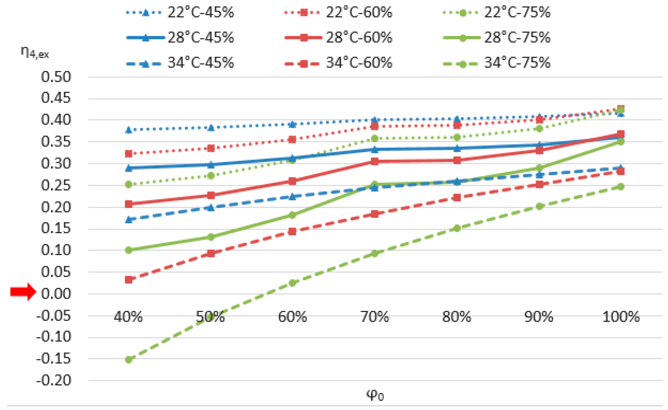
Equation (4) expresses the exergetic efficiency as ratio between the useful exergy output (i.e., the increase in thermal and chemical exergy of the air being cooled and dehumidified) and the exergy consumption (i.e., the reduction in the thermal and mechanical exergy of refrigerant, passing from state C to state D, plus the electric consumption to drive the fan). As an example, in Figure 3 the results obtained for a number of different scenarios are shown for the five rows coil, simulated as “clean”; results are plotted versus the relative humidity assumed for the ambient dead state, ϕ₀: in fact, according to Equation (3) the chemical fraction of air exergy (that increases across the coil due to the dehumidification) is highly sensitive to this parameter.

Looking at Figure 3, we may observe that:

-

When ϕ₀ increases from 40% to 100%, the exergetic performance also increases due to the higher value of chemical exergy of the dehumidified air: in fact, the higher the vapour content of the ambient “dead state” air, the higher the deviation from chemical equilibrium and the chemical exergy content of the low humidity air exiting at state “E-out” (see Figure 2);

-

At a given value of ϕ₀, the exergetic performance of the evaporator decreases for higher air inlet temperatures, because both the thermal exergy of the cooled air and the latent capacity of the coil decrease;

-

Negative values of the exergy efficiency were surprisingly obtained for low values of ϕ₀, when inlet air is very warm and humid (T_E-inl = 34 °C and ϕ_E-inl = 75%). This result is a consequence of the reduction in the chemical exergy of the cooled air, when moving across the coil: in fact, being dehumidified, the vapour content of air ω becomes closer to the reference vapour content ω₀ of ambient air and, according to Equation (3), the chemical exergy content of air decreases.

6. Fundamentals of the Adopted Thermoeconomic Diagnostic Technique

6.1. Generalities

Among the different thermoeconomic methodologies available, the Exergetic Cost theory [25] was adopted in this study, according to the innovative diagnostic technique presented in [17]. Explaining in details the fundamentals of this methodology is out of the scope of this paper, as an abundant literature on this method is available [26].

Let us indicate by F_i and P_i the fuel and the product of a generic plant component “i”, representing the consumed resources and the useful output of this component, respectively, both expressed in exergy units: in a typical productive component a material stream “m” reduces its exergy content from B_m^inlet to B_m^outlet (expressed in kW_ex) and the fuel F_i is calculated as “B_m^inlet − B_m^outlet”; similarly, if the productive scope of the same component is to increase the exergy of another fluid stream “n” from B_n^inlet to B_n^outlet, the product P_i will be expressed as “B_n^outlet − B_n^inlet”. Of course F_i > P_i due to the exergy destruction induced by any irreversible process occurring in the component.

Let us indicate as “residue flow” any exergy flow that is dissipated in a component, not representing its productive purpose; in some components, like the condenser of the examined refrigeration system, a residue flow (like the thermal exergy dissipated to cooling air) is the unique exergetic effect, because there is no apparent “exergetic product” P (i.e., no useful streams increase their exergy content across the component): such components are named “dissipative units”. Let us indicate by B_ij a generic exergy flow “produced” by the component “i” and “consumed” by the component “j”, and by R_ij a generic “residue” exergy flow “produced” by the component “i” (where it is physically dissipated) and “assigned” as an additional input to the component “j” [14]. Once introduced the “unit exergy consumption” κ_ij and the “residue generated per unit product” θ_ij:

$${\mathsf{\kappa }}_{\text{ij}}=\frac{{\mathrm{B}}_{\text{ij}}}{{\mathrm{P}}_{\mathrm{j}}},{\mathsf{\theta }}_{\text{ij}}=\frac{{\mathrm{R}}_{\text{ij}}}{{\mathrm{P}}_{\mathrm{j}}}$$

(5a,b)

and once defined for a generic i-th component an overall unit exergy consumption k_i and an overall unit residue generation r_i (with n indicating the number of components of the energy system):

$$k_i=\frac{{\mathrm{F}}_{\mathrm{i}}}{{\mathrm{P}}_{\mathrm{i}}}=\frac{{\displaystyle \sum _{\mathrm{j}=0}^{\mathrm{n}}{\mathrm{B}}_{\text{ji}}}}{{\mathrm{P}}_{\mathrm{i}}}={\displaystyle \sum _{\mathrm{j}=0}^{\mathrm{n}}{\mathsf{\kappa }}_{\text{ji}}},r_i=\frac{{\mathrm{R}}_{\mathrm{i}}}{{\mathrm{P}}_{\mathrm{i}}}=\frac{{\displaystyle \sum _{\mathrm{j}=0}^{\mathrm{n}}{\mathrm{R}}_{\text{ji}}}}{{\mathrm{P}}_{\mathrm{i}}}={\displaystyle \sum _{\mathrm{j}=0}^{\mathrm{n}}{\mathsf{\theta }}_{\text{ji}}}$$

(6a,b)

the overall increase of exergy destruction in the i-th component induced by the presence of faults is determined as sum of additional local exergy destruction due to irreversibility ΔI_i (where I_i = F_i−P_i) and additional residue generation ΔR_i:

$${\mathrm{\Delta }\mathrm{I}}_{\mathrm{i}}+{\mathrm{\Delta }\mathrm{R}}_{\mathrm{i}}=\mathsf{\Delta }\left[\left(k_{\mathrm{i}}-1\right){\mathrm{P}}_{\mathrm{i}}\right]+\mathsf{\Delta }\left(r_{\mathrm{i}}{\mathrm{P}}_{\mathrm{i}}\right)\cong \mathsf{\Delta }{k}_{\mathrm{i}}{\mathrm{P}}_{\mathrm{i}}\left(X^0\right)+\left[k_{\mathrm{i}}\left(X\right)-1\right]\cdot {\mathrm{\Delta }\mathrm{P}}_{\mathrm{i}}+\mathsf{\Delta }{r}_{\mathrm{i}}{\mathrm{P}}_{\mathrm{i}}\left(X^0\right)+r_{\mathrm{i}}\left(X\right)\cdot {\mathrm{\Delta }\mathrm{P}}_{\mathrm{i}}$$

(7)

In Equation (7) $X$ and $X^0$ respectively represent two sets of thermodynamic variables indicating the system operating under “design” (i.e., faults-free) and “faulty” conditions. Based on Equation (7), we may distinguish between:

-

Malfunction (or endogenous irreversibility), represented by the terms $\mathrm{\Delta }{k}_{\mathrm{i}}{\mathrm{P}}_{\mathrm{i}}\left(X^0\right)$ and $\mathrm{\Delta }{r}_{\mathrm{i}}{\mathrm{P}}_{\mathrm{i}}\left(X^0\right)$ and associated with increases in unit exergy consumptions or unit generation of residues in the i-th component:

$${\text{MF}}_{\mathrm{i}}={\text{MF}}_{\mathrm{i}}^{\text{(k)}}+{\text{MF}}_{\mathrm{i}}^{\text{(r)}}=\mathrm{\Delta }{k}_i{\mathrm{P}}_{\mathrm{i}}\left(X^0\right)+\mathrm{\Delta }{r}_i{\mathrm{P}}_{\mathrm{i}}\left(X^0\right)$$

(8)

-

Dysfunction (or exogenous irreversibility), induced in the i-th component by the malfunction of other components that provoke a variation ΔP_i in the production rate of component “i”:

$${\text{DF}}_{\mathrm{i}}={\displaystyle \sum _{i=1}^{\mathrm{n}}{\text{DF}}_{\text{ij}}^{\text{(k)}}}+{\displaystyle \sum _{i=1}^{\mathrm{n}}{\text{DF}}_{\text{ij}}^{\text{(r)}}}=\left[k_{\mathrm{i}}\left(X\right)-1\right]\cdot {\mathrm{\Delta }\mathrm{P}}_{\mathrm{i}}+r_{\mathrm{i}}\left(X\right)\cdot {\mathrm{\Delta }\mathrm{P}}_{\mathrm{i}}$$

(9)

The capability to distinguish between the additional exergy destruction in the i-th component provoked by faults occurring in the same component and those induced by malfunctions occurring in other components is the main added value of thermoeconomic diagnosis. Let us define for a generic i-th component a malfunction cost [8]:

$${\text{MF}}_{\mathrm{i}}^{*}={\text{MF}}_{\mathrm{i}}+{\displaystyle \sum _{\mathrm{j}=1}^{\mathrm{n}}\left({\text{DF}}_{\text{ji}}^{\left(\mathrm{k}\right)}+{\text{DF}}_{\text{ji}}^{\left(\mathrm{r}\right)}\right)}$$

(10)

According to Equation (10), ${\text{MF}}_{\mathrm{i}}^{*}$ represents the additional fuel consumption provoked by faults occurring in component “i”, and is calculated summing up the additional exergy destruction MF_i that these faults induce on the same component “i” (see Equation (7)) and the dysfunctions that these faults in component “i” induce in other components “j” (for j = 1 to n, with j ≠ i) [27].

When a reliable plant simulator is available, the efficiency of the diagnostic procedure in properly identifying a generic fault “j” and quantifying the additional energy consumption that it provokes can be evaluated by introducing an appropriate indicator, Ψ^{fault j}, defined as the ratio between the malfunction cost (i.e., the additional energy consumption induced by fault j, according to the estimation provided by the diagnostic technique) and the “fuel impact” ΔF_T, i.e., the actual additional energy consumption induced by fault j, calculated as difference between the energy consumption evaluated by the simulator in presence of fault j and the consumption evaluated when fault j is absent [17]. For an air-conditioning system, being the energy consumption related with the electricity W needed to drive the compressor and the fans, once indicated by {Ω} a generic set of multiple simultaneous faults that include “fault j” (i.e., a fault in the component “j”), Ψ^{fault j} is expressed as:

$${\mathsf{\Psi }}^{\text{fault j}}=\frac{{\text{MF}}_{\mathrm{j}}^{*}}{{\mathrm{\Delta }\mathrm{F}}_{\mathrm{T}}^{\left\{\text{fault j}\right\}}}=\frac{{\text{MF}}_{\mathrm{j}}^{*}}{{\mathrm{W}}^{\left\{\mathsf{\Omega }\right\}}-{\mathrm{W}}^{\left\{\mathsf{\Omega }-\text{fault j}\right\}}}$$

(11)

In the present paper only a single fault was considered, represented by evaporator fouling; then in Equation (11) {Ω} = {fault 4} was imposed, having been the evaporator identified as Component (4). As Ψ^{fault 4} represents the ratio between the “estimated additional energy consumption” and the “actual/exact additional energy consumption”, we may affirm that:

-

When Ψ^{fault 4} = 1 the diagnostic procedure perfectly quantifies the additional energy consumption provoked by the fouled evaporator (i.e., by “fault 4”);

-

When Ψ^{fault 4} > 1 or Ψ^{fault 4} < 1 the diagnostic procedure respectively over- or under-estimates the additional energy consumption provoked by “fault 4”.

6.2. On the Productive Structure Adopted to Perform the Thermoeconomic Diagnosis

In order to implement the methodology described in the previous subsection, the analyst must develop a “productive structure” of the energy system, i.e., a representation (either in graphical or tabular form) where the functional interactions between components are clearly identified. For each component the fuels, the products and the residue flows must be analytically expressed (in exergy units), based on a procedure that implies some arbitrary assumptions, thus making the reliability of results someway dependent on the experience of the analyst. For the examined air-conditioning system, a detailed analysis was performed in [17] identifying a reliable productive structure that has been graphically presented in the cited paper. In the present article, the same productive structure was adopted, which is here presented by the so-called Fuels-Products-Residues Table, see

Table 2. Fuel-Product-Residue table of the examined refrigeration system, according to the procedure proposed in [17].

-	F0	F1	F2	F3	F4	R1	R2	R3	R4
P0	0	$\mathsf{\alpha }\cdot {\mathrm{W}}_1$	$\mathsf{\alpha }\cdot {\mathrm{W}}_2$	0	$\mathsf{\alpha }\cdot {\mathrm{W}}_4$	0	0	0	0
P1	0	0	$\begin{array}{l}\alpha \cdot \mathrm{\Delta }{\mathrm{B}}_2^{\text{total}}\left(X\right)-\mathrm{\Delta }{\mathrm{B}}_2^{\text{total}}\left(X^0\right)+\\ a_2\cdot \mathrm{\Delta }{\mathrm{B}}_3^{*}\end{array}$	${\mathrm{\Delta }\mathrm{B}}_3^{\mathrm{P}}\left(X^o\right)$	$\begin{array}{l}\alpha \cdot \mathrm{\Delta }{\mathrm{B}}_4^{\text{total}}\left(X\right)+a_4\cdot \mathrm{\Delta }{\mathrm{B}}_3^{*}-\\ \text{r }\left(X^0\right)\cdot \mathrm{\Delta }{\mathrm{B}}_4^{\mathrm{T}}\left(X^0\right)\end{array}$	$a_1\cdot {\mathrm{\Delta }\mathrm{B}}_3^{*}$	0	0	0
P2	0	0	0	0	0	$\begin{array}{l}\left(1-\mathrm{r}\right)\cdot \mathrm{\Delta }{\mathrm{B}}_2^{\text{total}}\left(X^0\right)+\\ c_1\cdot \mathrm{\Delta }{\mathrm{B}}_2^{*}\end{array}$	$c_2\cdot {\mathrm{\Delta }\mathrm{B}}_2$	$\left(1-\mathrm{r}\right)\cdot {\mathrm{\Delta }\mathrm{B}}_2^{\mathrm{T}}\left(X^0\right)$	$c_4\cdot {\mathrm{\Delta }\mathrm{B}}_2^{*}$
P3	0	0	${\mathrm{\Delta }\mathrm{B}}_2^{\text{total}}\left(X^o\right)$	0	0	0	0	0	0
P4	$\mathsf{\alpha }\cdot {\mathrm{\Delta }\mathrm{B}}_4^{\text{air}}$	0	0	0	$\text{r }\left(X^0\right)\cdot {\mathrm{\Delta }\mathrm{B}}_4^{\mathrm{T}}\left(X^0\right)$	0	0	0	0
Total	$\mathsf{\alpha }\cdot {\mathrm{\Delta }\mathrm{B}}_4^{\text{air}}$	$\mathsf{\alpha }\cdot {\mathrm{W}}_1$	$\alpha \cdot \left[{\mathrm{W}}_2+{\mathrm{\Delta }\mathrm{B}}_2^{\text{total}}\left(X\right)\right]+a_2\cdot {\mathrm{\Delta }\mathrm{B}}_3^{*}$	${\mathrm{\Delta }\mathrm{B}}_3^{\mathrm{P}}\left(X^0\right)$	$\alpha \cdot {\mathrm{\Delta }\mathrm{B}}_4^{\text{total}}\left(X\right)+a_4\cdot {\mathrm{\Delta }\mathrm{B}}_3^{*}$	$\begin{array}{l}\left(1-\mathrm{r}\right)\cdot \mathrm{\Delta }{\mathrm{B}}_2^{\text{total}}\left(X^0\right)+\\ c_1\cdot \mathrm{\Delta }{\mathrm{B}}_2^{*}+a_1\cdot \mathrm{\Delta }{\mathrm{B}}_3^{*}\end{array}$	$c_2\cdot {\mathrm{\Delta }\mathrm{B}}_2^{*}$	$\left(1-\mathrm{r}\right)\cdot {\mathrm{\Delta }\mathrm{B}}_2^{\mathrm{T}}\left(X^0\right)$	$c_4\cdot {\mathrm{\Delta }\mathrm{B}}_2^{*}$

. Avoiding to enter into details about the rational of each expression in Table 2, some key-points can be clarified:

-

In Table 2, for each component from 1 to 4 (following the notation adopted in Figure 2), the fuels consumed and the residues generated (which are described as “additional inputs to the components”, following a well-established criterion formulated by Valero et al.), can be found in the different columns. Both the ambient interacting with the air-conditioning system (i.e., the cooled ambient and the surrounding environment) were considered a virtual component “0”. In the rows, conversely, we may identify the corresponding products. All flows were obviously expressed in exergy units (i.e., in kW_ex);

-

Three main symbols are used in Table 2 for the exergy associated with refrigerant flows inside each generic component “i”, that are ΔB_i^P, ΔB_i^T and ΔB_i^total. While ΔB_i^total indicates the variation of the total exergy content of the refrigerant flow across the component “i”, ΔB_i^P and ΔB_i^T represent the aforementioned two complementary fractions of this variation, respectively related with “mechanical” (or pressure-dependent, or “thermobaric”) and “thermal” (or temperature-dependent, or “thermoambient”) deviation between the refrigerant state and the reference dead state [28]; the exergetic cost theory, in fact, provides more accurate and easy-to-interpret results when based on physical exergy flows split into mechanical and thermal terms;

-

All the exergy flow variations across a component calculated in the generic “faulty” operating condition (identified by the set of thermodynamic parameters $X$) were multiplied by a factor α, named “cooling capacity factor”, calculated as ratio between the exergetic product of the evaporator respectively in the “faults-free” and in the “faulty” operating conditions:

$$\mathsf{\alpha }=\frac{{\left({\mathrm{\Delta }\mathrm{B}}_4^{\text{total,air}}\right)}_{\text{clean coil}}}{{\left({\mathrm{\Delta }\mathrm{B}}_4^{\text{total,air}}\right)}_{\text{dirty coil}}}$$

(12)

This approach is useful to reflect the actual operation of the system (governed by control devices), which does not response to malfunctions modifying the final product (i.e., reducing its capacity) at a constant energy consumption rate, but rather increases its energy consumption in order to maintain a constant product and balance the load [17].

Some peculiar terms can be found in Table 2, that include two variables ΔB₂^* and ΔB₃^* calculated basing on the following Equations (13) and (14), and respectively indicating the increase in the exergy variations of refrigerant across the condenser and the thermal expansion valve, when compared between the “faulty” and the “design” operating conditions (respectively indicated by the set of thermodynamic parameters $X$ and $X^0$):

$${\mathrm{\Delta }\mathrm{B}}_2^{*}={\mathrm{\Delta }\mathrm{B}}_2^{\text{total}}\left(X\right)-{\mathrm{\Delta }\mathrm{B}}_2^{\text{total}}\left(X^0\right)$$

(13)

$${\mathrm{\Delta }\mathrm{B}}_3^{*}={\mathrm{\Delta }\mathrm{B}}_3^{\text{total}}\left(X\right)-{\mathrm{\Delta }\mathrm{B}}_3^{\text{total}}\left(X^0\right)$$

(14)

According to a methodology well explained in [17], the aforementioned additional exergy destructions ΔB₂^* and ΔB₃^* were allocated (as additional fuels or residue flows, see Table 2) to the compressor, the condenser and the evaporator, based on appropriate distribution ratios (a₁, a₂ and a₄ are used to allocate the term ΔB₃^*, c₁, c₂ and c₄ to allocate the term ΔB₂^*). This approach and the procedure to calculate the distribution ratios have been presented and validated in [17] and describing it in further details is out of the scope of the present paper. It is here sufficient to clarify that the proposed approach represents an alternative solution to a well-known problem in thermoeconomic diagnosis: if the diagnostic procedure identifies a faulty component “i” by detecting increases Δk_i > 0 in its unit exergy consumption, such increases should be filtered from the fraction induced by changes in the operational condition of the component provoked by modifications occurring in other components. In fact, assuming an increase in the unit exergy consumption Δk_i > 0 as a direct measure of a local fault in component “i” has been proven wrong due to two different effects:

(1)

The intervention of control systems, aimed at restoring pre-fixed values for some specific parameters, leads the plant toward a “modified operating condition” which in its turn induces changes in the unit exergy consumption of the components. Filtering these effects can be achieved by identifying (through a simulator-aided procedure) a “free condition”, characterized by the same position of the governing parameters (as the design condition) but containing the anomalies occurring at the actual operating condition [29];

(2)

The dependence of the efficiency curves of components on the operating condition influences the unit exergy consumption. In fact, when a unit changes its operating point, generally its efficiency changes, inducing the presence of a malfunction. The elimination of these induced effects is complex and requires the use of a thermodynamic model for each component to predict its response to changes in the operating conditions [11,30].

In the literature several approaches have been proposed to distinguish between intrinsic malfunctions (those induced by faults located in the component) and the induced malfunctions (related with the aforementioned effect) [10], since the aforementioned effects have been proven to influence negatively the efficiency of thermoeconomic diagnostic techniques in detecting several faults, like those occurring in steam generators. In this paper the aforementioned approach, proposed in [17] and based on the distribution of the additional exergy destructions ΔB₂^* and ΔB₃^* by appropriate coefficients “a₁, a₂, a₄” and “c₁, c₂, c₄” represents an alternative route to pursue this same objective. In fact, the exergetic performance of components in refrigeration systems is even less stable and more sensitive to malfunctions than the one of components in steam power plants. Once expressed any exergy input B_ij to a generic component “j” as a function of m thermodynamic variables that influence its operation:

B_ij = B_ij (x₁, x₂, …, x_m)

(15)

with {x₁, x₂, …, x_m} $\in$ $X$, the values of $\partial {\mathrm{B}}_{\text{ij}}/\partial x_l$ (l = 1, …, m) are unusually high, compared to the typical values observed in steam power cycles. It is thus evident the extreme importance of a implementing some technique to filter not only the effects of efficiency curves and controls, but also the influence of the ambient conditions: consequently both the diagnosed operating condition and the “design/reference” one must refer to the same temperature and (less importantly) relative humidity of the cooling air entering the condenser! Actually, the procedure proposed in [17] and adopted in this paper essentially filters the induced malfunctions (i.e., the changes in exergetic performance) occurring in the condenser and the flow metering device and provoked by the most common faults in air conditioning systems. Unfortunately, eventual induced malfunctions in the compressor are not filtered; however, ex-post analyses have shown that the effects induced by evaporator fouling on this component were very small for all the examined air inlet conditions and coil geometries:

$$\mathrm{\Delta }{k}_1={\displaystyle \sum _{j=0}^4\mathrm{\Delta }{\kappa }_{j1}\cong 0.01-0.03}$$

(16)

6.3. On the Best Settings to Perform the Thermoeconomic Diagnosis

Before implementing the thermoeconomic diagnosis procedure, some critical arguments must be addressed. First of all, let us observe that in order to correctly detect the evaporator coil as “dirty or fouled” by a thermoeconomic technique, the exergetic performance of this component should get worse in the presence of fouling. While it can be easily predicted that the cooling capacity of the coil reduces, when measuring the performance in exergetic units the result is harder to predict. In order to focus on this critical point, in

Table 3. Exergetic parameters calculated for the 5-rows “clean” coil in all the inlet conditions.

T (°C)	ϕ (%)	Gair (kg/s)	${\mathrm{\Delta }\mathrm{b}}_4^{\text{T,air}}$ (kJex/kg)	${\mathrm{\Delta }\mathrm{b}}_4^{\text{C,air}}$ (kJex/kg)	${\mathrm{\Delta }\mathrm{B}}_4^{\text{T,air}}$ (kWex)	${\mathrm{\Delta }\mathrm{B}}_4^{\text{C,air}}$ (kWex)	${\mathrm{\Delta }\mathrm{B}}_4^{\text{total,air}}$ (kWex)
22	45	7.1	0.82	0.15	5.85	1.06	6.91
22	60	6.9	0.66	0.36	4.58	2.50	7.08
22	75	6.8	0.51	0.50	3.49	3.41	6.90
25	45	7.0	0.73	0.19	5.11	1.30	6.41
25	60	6.8	0.57	0.39	3.86	2.62	6.48
25	75	6.7	0.42	0.50	2.83	3.34	6.18
28	45	6.9	0.63	0.22	4.30	1.49	5.79
28	60	6.7	0.47	0.40	3.11	2.65	5.76
28	75	6.6	0.33	0.47	2.16	3.14	5.31
31	45	6.7	0.51	0.24	3.41	1.60	5.01
31	60	6.5	0.35	0.38	2.31	2.49	4.80
31	75	6.4	0.23	0.43	1.48	2.74	4.22
34	45	6.6	0.38	0.24	2.50	1.57	4.07
34	60	6.5	0.23	0.34	1.52	2.18	3.70
34	75	6.3	0.13	0.35	0.83	2.19	3.02

and

Table 4. Exergetic parameters calculated for the 5-rows “dirty” coil in all the inlet conditions.

T (°C)	ϕ (%)	Gair (kg/s)	${\mathrm{\Delta }\mathrm{b}}_4^{\text{T,air}}$ (kJex/kg)	${\mathrm{\Delta }\mathrm{b}}_4^{\text{C,air}}$ (kJex/kg)	${\mathrm{\Delta }\mathrm{B}}_4^{\text{T,air}}$ (kWex)	${\mathrm{\Delta }\mathrm{B}}_4^{\text{C,air}}$ (kWex)	${\mathrm{\Delta }\mathrm{B}}_4^{\text{total,air}}$ (kWex)
22	45	5.77	0.96	0.26	5.53	1.50	7.03
22	60	5.53	0.79	0.49	4.39	2.73	7.12
22	75	5.55	0.62	0.64	3.43	3.54	6.97
25	45	5.63	0.84	0.29	4.75	1.66	6.41
25	60	5.47	0.68	0.53	3.72	2.91	6.63
25	75	5.38	0.52	0.64	2.80	3.45	6.25
28	45	5.54	0.74	0.35	4.10	1.93	6.02
28	60	5.40	0.56	0.54	3.02	2.89	5.91
28	75	5.31	0.41	0.62	2.16	3.29	5.45
31	45	5.31	0.62	0.39	3.41	1.60	5.01
31	60	5.17	0.62	0.39	3.28	2.10	5.37
31	75	5.08	0.44	0.54	2.27	2.78	5.05
34	45	5.27	0.30	0.57	1.51	2.90	4.41
34	60	5.11	0.47	0.39	2.46	2.08	4.54
34	75	5.02	0.30	0.49	1.54	2.52	4.07

the exergetic results concerning the evaporator are presented, for the 5 rows-coil and the 15 examined air-inlet conditions (assuming ϕ₀ = 100%), and for the “clean” and the “dirty or fouled” coil, respectively.

From a simple comparison between the two tables, we may observe that:

-

The “exergetic useful product” of the evaporator, that is represented by the increase ${\mathrm{\Delta }\mathrm{B}}_4^{\text{total,air}}$ in the total exergy of the cooled air when it passes across the coil (last column in the tables), is always higher for the “fouled” coil compared to the “clean” one. Then, due to the analytical expression of total exergy, although the presence of fouling produces a reduction in the cooling capacity, expressed as:

$${\stackrel{\cdot }{\mathrm{Q}}}_{\text{cooling}}={\mathrm{G}}^{\text{air}}\cdot \left({\mathrm{h}}_{\mathrm{E}-\text{int}}-{\mathrm{h}}_{\mathrm{E}-\text{out}}\right)$$

(17)

it improves the exergetic performance of the coil, by leading to higher values of ${\mathrm{\Delta }\mathrm{B}}_4^{\text{total,air}}$;

-

The origin of this peculiar trend becomes evident when looking at the 3rd–7th columns in the tables. In fact, due to the reduction in the air flow rate G^air, each kg of air undergoes a more intense cooling and dehumidification process, as testified by the relevant increases of both ${\mathrm{\Delta }\mathrm{b}}_4^{\text{T,air}}$ and ${\mathrm{\Delta }\mathrm{b}}_4^{\text{C,air}}$ when passing from the “clean” to the “fouled” coil. However, the increase in the specific thermal exergy of air ${\mathrm{\Delta }\mathrm{b}}_4^{\text{T,air}}$ is moderate, thus leading to a reasonable decrease in the performance of the coil (passing from the “clean” to the “fouled” condition), when measured in terms of “thermal exergy transferred to the fluid”: ${\mathrm{\Delta }\mathrm{B}}_4^{\text{T,air}}={\mathrm{G}}^{\text{air}}\cdot {\mathrm{\Delta }\mathrm{b}}_4^{\text{T,air}}$. On the contrary, when we examine the behaviour of the fraction of the “exergetic product” related with dehumidification and measured in terms of chemical exergy, we may observe an opposite behaviour: the increase in the specific chemical exergy ${\mathrm{\Delta }\mathrm{b}}_4^{\text{C,air}}$ when passing from the “clean” to the “fouled” coil prevails on the effect of reduction in the air mass flow rate, thus leading to an increase in the “chemical exergy rate transferred to the fluid” ${\mathrm{\Delta }\mathrm{B}}_4^{\text{C,air}}={\mathrm{G}}^{\text{air}}\cdot {\mathrm{\Delta }\mathrm{b}}_4^{\text{C,air}}$.

As a result of the above argument, it may be easily predicted that any thermoeconomic diagnostic technique applied by using “total exergy” flows would be inefficient, since a “dirty or fouled” coil misleadingly seems to perform better than a “clean” coil, when its performance is measured in terms of “total exergy”. Also, we recognized that this distortion is provoked by the anomalous behaviour of chemical exergy. Then, a minor change was introduced in the thermoeconomic productive structure presented in Table 2, consisting of replacing, as a useful exergetic product of the evaporator (cell “P₄-F₀” in the Fuel-Product-Residue table), the total exergy ${\mathrm{\Delta }\mathrm{B}}_4^{\text{total,air}}$ acquired by the cooled air with the thermal fraction only, ${\mathrm{\Delta }\mathrm{B}}_4^{\text{T,air}}$, of the exergy acquired by air passing from state “E-inl” to “E-out”. Consequently, a new definition of the “cooling capacity factor” α was formulated (modified compared to Equation (12)):

$$\mathsf{\alpha }=\frac{{\left({\mathrm{\Delta }\mathrm{B}}_4^{\text{T,air}}\right)}_{\text{clean coil}}}{{\left({\mathrm{\Delta }\mathrm{B}}_4^{\text{T,air}}\right)}_{\text{dirty coil}}}$$

(18)

This expression of the cooling capacity factor has another advantage: it better reflects the logics of automatic control of air-conditioning units. For instance, in case of thermostatic control “on-off” of the compressor, the control unit responds to eventual decreases of the cooling capacity of the system (detected basing only on measurements of temperature) by increasing the duration of “on-cycles” to maintain the same average cooling capacity needed to balance the load.

According to the discussion above, we expected that passing from the use of “total air exergy” to the use of only the “thermal fraction of air exergy”, the performance of the diagnostic technique would have been improved due to the fact that the presence of a dirty coil now produced a detectable reduction in the “exergy product” of the evaporator. In simple words, we expected a better performance of the diagnostic technique when the cooling capacity factor α is higher than 1. In

Table 5. Cooling capacity factors for all the coil geometries and air inlet conditions.

	${\left(\mathsf{\alpha }\right)}_{\text{Eq.12}}=\frac{{\left({\mathrm{\Delta }\mathrm{B}}_4^{\text{total, air}}\right)}_{\text{clean coil}}}{{\left({\mathrm{\Delta }\mathrm{B}}_4^{\text{total, air}}\right)}_{\text{dirty coil}}}$			${\left(\mathsf{\alpha }\right)}_{\text{Eq.18}}=\frac{{\left({\mathrm{\Delta }\mathrm{B}}_4^{\text{T, air}}\right)}_{\text{clean coil}}}{{\left({\mathrm{\Delta }\mathrm{B}}_4^{\text{T, air}}\right)}_{\text{dirty coil}}}$
Air Inlet Condition	3 Rows	5 Rows	7 Rows	3 Rows	5 Rows	7 Rows
22 °C-45%	0.91	0.99	0.97	0.98	1.06	1.10
22 °C-60%	0.99	0.99	1.00	1.02	1.04	1.07
22 °C-75%	1.00	0.98	1.01	0.99	1.02	1.04
25 °C-45%	0.98	1.01	0.96	1.03	1.07	1.11
25 °C-60%	0.99	0.98	0.99	1.02	1.04	1.07
25 °C-75%	0.98	0.98	1.00	0.99	0.99	1.03
28 °C-45%	0.95	0.97	0.95	1.02	1.05	1.09
28 °C-60%	0.98	0.98	0.97	0.99	1.03	1.17
28 °C-75%	0.97	0.98	0.99	0.98	0.99	1.02
31 °C-45%	0.94	0.93	0.90	0.99	1.04	1.09
31 °C-60%	0.95	0.95	0.93	0.99	1.02	1.05
31 °C-75%	0.96	0.96	0.93	0.96	0.98	0.99
34 °C-45%	0.92	0.90	0.86	0.97	1.02	1.07
34 °C-60%	0.93	0.92	0.90	0.94	0.98	1.02
34 °C-75%	0.92	0.93	0.88	0.89	0.93	0.95

a synthetic comparison of the values of α calculated according to Equations (12) and (18) (i.e., respectively based on the total air exergy and on its thermal fraction only) is presented, for ϕ₀ = 100%, for the three examined coil geometries and the 15 scenarios assumed as concerns air inlet conditions.

In Table 5 the values of the cooling capacity factor higher than 1 are highlighted by using bold black characters and light grey back color. We may observe that passing from the “total air exergy” (α calculated according to Equation (12)) to the “thermal fraction only of exergy” (α calculated according to Equation (18)), the capability of the thermoeconomic technique to correctly diagnose a fouled coil could be expected to improve significantly. In particular, while in this improved scenario the values of α remained often lower than 1 for the 3-rows coil, much more promising results were found for the five and specially the seven row coils, which achieved α > 1, respectively, for 10 and 13 scenarios out of the 15 ones examined as concerns the coil air inlet conditions.

Then, in the next section, the results of the thermoeconomic diagnosis will be shown with reference to a procedure based on the use of “thermal exergy transferred to the cooled air” assumed as the unique useful product of the evaporator coil.

7. Analysis of the Results Achieved by Thermoeconomic Diagnosis

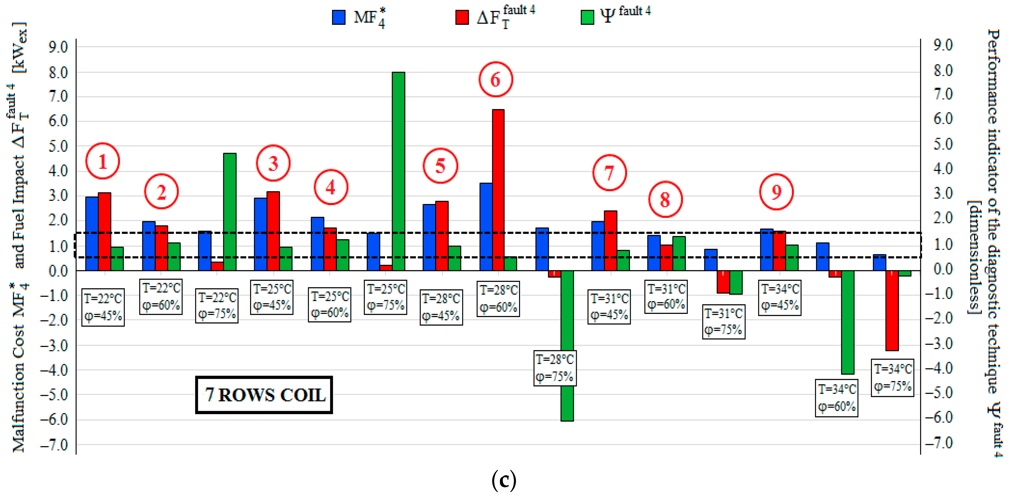
Once presented in the previous sections all the methodological aspects and some crucial settings needed to make the procedure potentially reliable, the thermoeconomic diagnosis was performed by imposing for all the scenarios and coil geometries a “heavy fouling” condition (corresponding to a decrease in the air face velocity from 2.7 m/s down to 2.1 m/s) and verifying whether or not the diagnostic procedure was able to correctly identify the evaporator coil as “dirty or fouled”. In this section the results obtained for all the examined scenarios will be presented and discussed.

In Figure 4a–c three series of results are shown, respectively for the three, five and seven row coils and for all the examined scenarios as concerns the coil air inlet conditions:

-

The term ${\text{MF}}_4^{*}$ indicates the estimation of additional exergy consumption induced by evaporator fouling, according to the diagnostic procedure proposed in [17] and described by the tabular productive structure presented in Table 2;

-

The term ΔF_T represents the actual additional exergy consumption provoked by evaporator fouling (at a fixed exergy production rate). This term, that usually represents an unknown value when diagnosing a real plant, is in our case known because the “faulty” scenarios have been numerically simulated, thus making available the correct value to benchmark the performance of the diagnostic technique;

-

The performance indicator Ψ^{fault 4} represents the ratio between the two above terms, which assesses the reliability of the technique in quantifying the additional consumption.

Looking at Figure 4a–c, we may observe that:

(1)

the vast majority of cases, i.e., for most of the combinations of boundary conditions (inlet air temperature and humidity) and geometry (i.e., coil depth), the term ${\text{MF}}_4^{*}$ is positive; in all these cases the thermoeconomic diagnosis provides a correct response “from a qualitative viewpoint”, since due to the resulting positive malfunction cost it can provide an alert signal for the apparent presence of fouling at the evaporator (component “4”). Only in three cases, and in particular for the three row coil and in presence of very high air inlet temperature and relative humidity (i.e., in case of very high absolute humidity of the inlet air), the technique fails in detecting the evaporator as “probably fouled”, as evident from the ${\text{MF}}_4^{*}$ < 0;

(2)

In a number of cases (more frequently for the three row coil, rarely for the five and seven row ones) the term ΔF_T is negative, thus resulting in a consequently negative value of the performance indicator Ψ^{fault 4}. In such conditions the use of “exergy” as a basis to identify malfunctions reveals inadequate, since the dirty/fouled coil appears “more exergetically efficient” than the clean coil, thus leading to an evident inconsistency. This condition may be observed to occur for the same set of conditions that in Table 5 had been observed to achieve the unsatisfactory condition ${\left(\mathsf{\alpha }\right)}_{\text{Eq.18}}<1$ . Since most of these cases occur (for any coil geometry) at high relative humidities of inlet air (i.e., when a large fraction of the coil is wet), we may conclude that the use of “exergy-based” diagnostic techniques is favoured (even when chemical exergy of dehumidified air is excluded from the analysis, as in our case) when air with a quite low relative humidity enters the coil, i.e., when most of the rows operate in dry conditions;

(3)

Once excluded the aforementioned cases where ΔF_T < 0 occurs, let us look at the numerical value assumed by the performance indicator Ψ^{fault 4}, in order to assess whether or not the diagnostic technique is efficient in quantifying the additional consumption induced by evaporator fouling. Let us assume as a good performance indication, from a “quantitative viewpoint”, the condition “0.5 < Ψ^{fault 4} < 1.5”, identified by the hatched bold line contour in Figure 3a–c; in fact, in such cases we are sure that $0.5{\mathrm{\Delta }\mathrm{F}}_{\mathrm{T}}^{\text{fault4}}<{\text{MF}}_4^{*}<1.5{\mathrm{\Delta }\mathrm{F}}_{\mathrm{T}}^{\text{fault4}}$ and that ${\text{MF}}_4^{*}$ (the output value of the diagnostic technique) represents a more or less reasonable estimation of the actual additional consumption ${\mathrm{\Delta }\mathrm{F}}_{\mathrm{T}}^{\text{fault4}}$ induced by the dirty coil (this value being, as said above, unknown in any real world application). The cases where the above condition is satisfied and the technique achieves a quite appreciable “quantitative” performance are identified by a red circle and numerated consecutively in Figure 4a–c. It is evident that for the five and seven row coils the diagnostic technique performs well in a high number of cases, and in particular in most of the cases with relative humidity between 45% and 60% (which represent the largely most common situation in civil uses of air conditioning); for a 75% relative humidity, the diagnostic procedure has a much poorer performance, with a relevant overestimation of the additional exergy consumption provoked by evaporator fouling. On the contrary, the performance of the diagnostic technique is always poor for the system with a three row coil, with frequent overestimation of the impact of evaporator fouling.

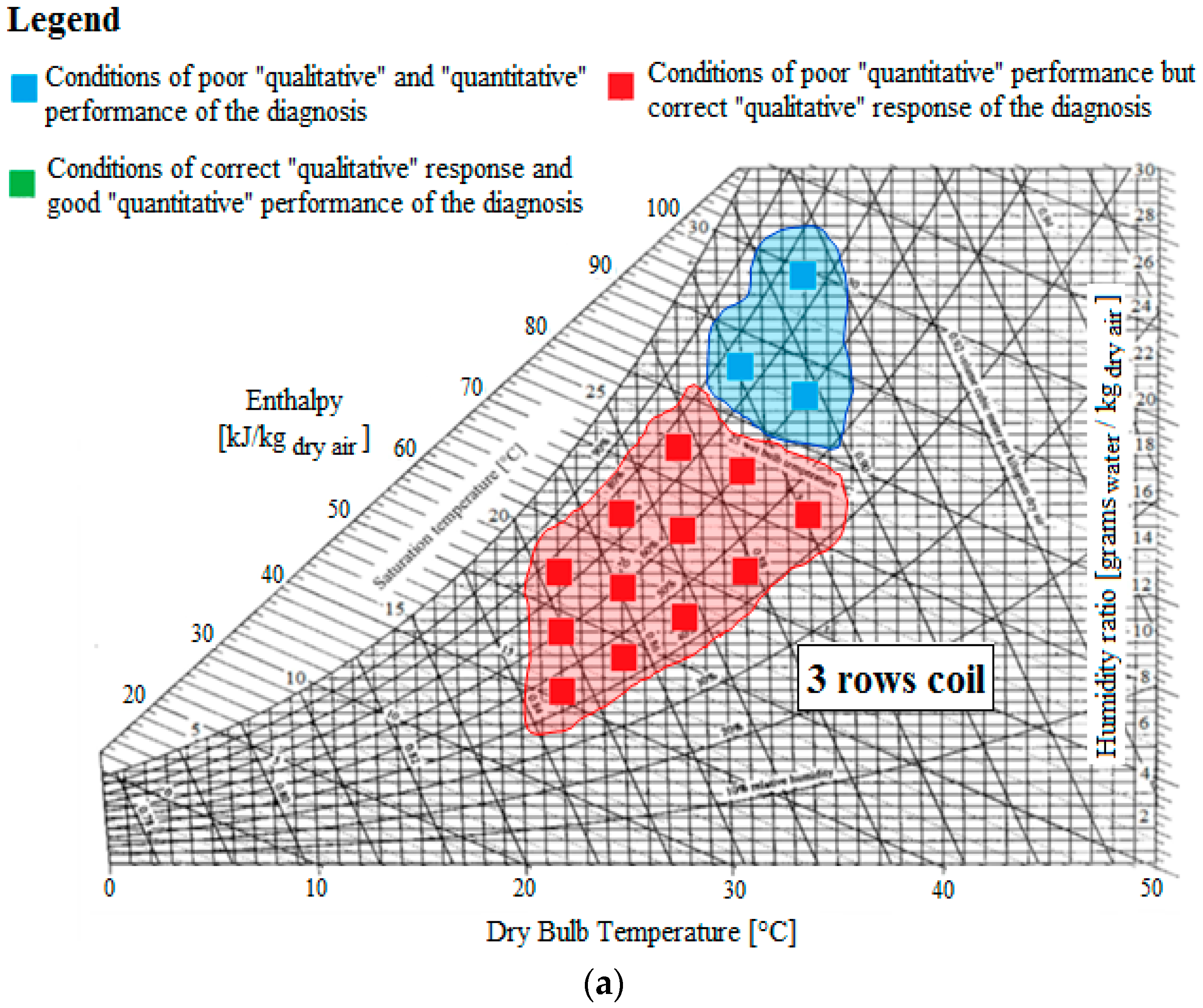
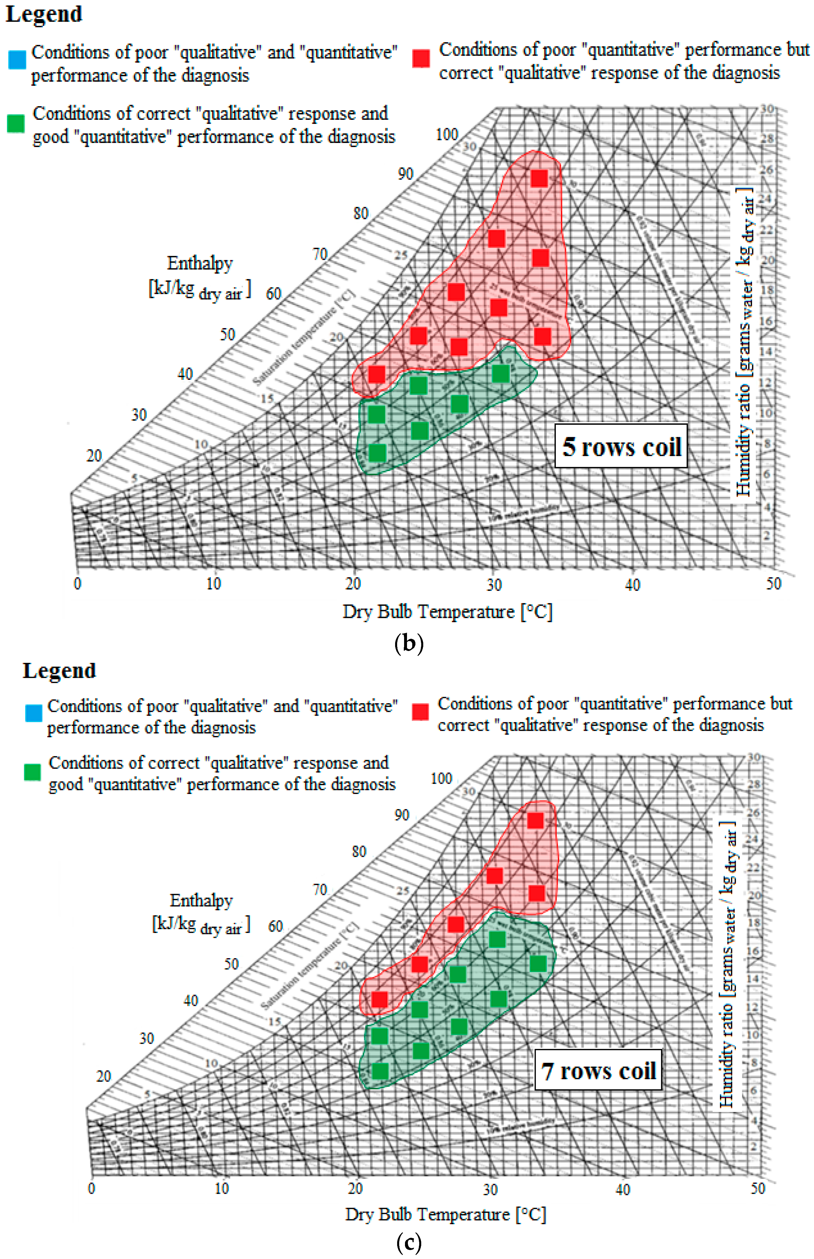
The relation between the sensitivity of performance of the diagnostic technique to the coil geometry and to the inlet air conditions appears much more clear and intuitive in Figure 5a–c. Here the three aforementioned levels of performance, based on a qualitative aspect (related with the capability to detect the dirty coil condition) and a quantitative aspect (related with the capability of the technique to provide a reasonable estimation of the additional energy consumption induced by the dirty coil), are mapped over a psychrometric chart.

This representation allows to observe much more intuitively that the thermoeconomic diagnostic technique performs worse whenever the air entering the cooling coil has a high absolute humidity.

An interpretation of the poor performance of the diagnostic technique in certain operating conditions is here provided. As stated in Section 6.2, the effectiveness of the technique used to filter induced malfunctions (so as to focus only on intrinsic ones) is of utmost importance for the reliability of thermoeconomic diagnosis of refrigeration systems. The adopted filtering technique, that uses two sets of distribution ratios (“a₁, a₂, a₄” and “c₁, c₂, c₄”) to allocate respectively the effects induced by malfunctions on the expansion valve and the condenser, was implemented using specific values of these ratios calculated in [17] for a specific geometry (five row coil) and a specific set of operating conditions (in particular assuming t = 27 °C and ϕ = 65% as air inlet conditions to the evaporator coil). One of the limits of the method can be related with the poor performance of the technique used to filter these induced malfunctions, whenever the diagnosed geometry and operating condition significantly differ from the reference geometry/condition used in [17] to fix the distribution ratios. From this perspective, future advances of the technique could be aimed at calibrating the optimal values of the distribution ratios to be used for each specific coil geometry and interval of operating conditions (i.e., for each specific region of the psychrometric chart in Figure 5). Another possible limit of the technique is related with the volatility of the exergy function when air is intensely dehumidified across the coil, i.e., when most of its surface operates in wet conditions; in order to overcome this limit, more accurate thermodynamic models will be probably needed to filter efficiently the malfunctions induced by changes in the exergy performance.

The proposed analysis revealed that in general the performance of the diagnosis is very sensitive to all the examined parameters. This result is very relevant; in fact, the particular operating conditions tested in [17] had led to an excellent diagnostic performance of the technique, thus making this pioneering technique seem a ready-to-use and reliable methodology, which could be expected to have potential for testing in industrial components. Conversely, the results of this study verified that: (i) the methodology is not robust, since its performance is extremely sensitive to the operating conditions (due to the particular behaviour of the function “exergy”) and (ii) it is very likely that exergy-based diagnostic techniques should necessarily be designed, in the field of refrigeration and air-conditioning, paying great attention to the specific conditions expected during the plant lifetime operation.

8. Conclusions

In this paper the robustness of thermoeconomic diagnosis for the detection of malfunctions in direct-expansion air-conditioning units was investigated. The sensitivity of performance to a number of different variables was assessed, focusing the attention on the thermodynamic conditions of the coil inlet air to be cooled and dehumidified, the “dead state” humidity assumed and the coil geometry.

The preliminary exergy analysis revealed that due to the analytical expression of chemical and thermal exergy, the assumption of the “total exergy of the cooled air” as useful output of the evaporator coil can lead to misleading result; in particular, based on the total exergy performance, the unit may erroneously appear to work more efficiently with a dirty coil, compared to the “reference case” of clean coil.

Once properly implemented the diagnostic technique on the basis of the “thermal fraction only” of air exergy, the performance of the methodology revealed highly sensitive to both the inlet air conditions and to the coil geometry. In particular, it resulted very efficient both in detecting the faulty unit and in quantifying the additional energy consumption induced by fouling when the air entering the coils has a low absolute humidity (i.e., not to high values of temperature and relative humidity); also, the efficiency of the technique resulted to increase when coils with higher depth are considered. These results, mapped on a psychrometric chart, allowed to distinguish between regions where a performance of the diagnosis can be expected and other regions where the thermoeconomic diagnosis performs poorly.

As a general conclusion, it can be said that the pioneering use of thermoeconomic diagnosis for air-conditioning applications requires great expertise of the analyst, which should in general design the whole procedure being aware of the conditions the plant will most likely encounter during its operation.

References

1. Eurovent Certification Program. Available online: http://www.eurovent-certification.com (accessed on 14 December 2015).
2. Devecioğlua, A.G.; Oruç, V. Characteristics of Some New Generation Refrigerants with Low GWP. Energy Procedia 2015, 75, 1452–1457. [Google Scholar] [CrossRef]
3. Bergles, A.E. EXHFT for fourth generation heat transfer technology. Exp. Therm. Fluid Sci. 2002, 26, 335–344. [Google Scholar] [CrossRef]
4. Breuker, M.G.; Braun, J.E. Common Faults and Their Impacts for Rooftop Air Conditioners. HVAC&R Res. 1998, 4, 303–318. [Google Scholar]
5. McKellar, M.G. Failure Diagnosis for a Household Refrigerator. Master’s Thesis, Purdue University, West Lafayette, IN, USA, 1987. [Google Scholar]
6. Rossi, T.M.; Braun, J.E. A statistical rule-based fault detection and diagnostic method for vapor compression air conditioners. HVAC&R Res. 1997, 3, 19–37. [Google Scholar]
7. Li, H.; Braun, J.E. Decoupling features and virtual sensors for diagnosis of faults in vapor compression air conditioners. Int. J. Refrig. 2007, 30, 546–564. [Google Scholar] [CrossRef]
8. Valero, A.; Correas, L.; Zaleta, A.; Lazzaretto, A.; Verda, V.; Reini, M.; Rangel, V. On the thermoeconomic approach to the diagnosis of energy system malfunctions: Part 2. Malfunction definitions and assessment. Energy 2004, 29, 1889–1907. [Google Scholar] [CrossRef]
9. Verda, V. Thermoeconomic Analysis and Diagnosis of Energy Utility Systems—From Diagnosis to Prognosis. Int. J. Thermodyn. 2004, 7, 73–83. [Google Scholar]
10. Usón, S.; Valero, A. Application of Quantitative Causality Analysis to the Quantification of Intrinsic and Induced Effects in the Thermoeconomic Diagnosis of a Coal-fired Power Plant. Int. J. Thermodyn. 2009, 12, 61–67. [Google Scholar]
11. Verda, V. Accuracy level in thermoeconomic diagnosis of energy systems. Energy 2006, 31, 3248–3260. [Google Scholar] [CrossRef]
12. Frangopoulos, C.A. Thermoeconomic Functional Analysis—A Method for the Optimal Design or Improvement of Complex Energy Systems. Ph.D. Thesis, Georgia Institute of Technology, Atlanta, GA, USA, 1983. [Google Scholar]
13. D’Accadia, M.D.; de Rossi, F. Thermoeconomic analysis and diagnosis of a refrigeration plant. Energy Convers. Manag. 1998, 39, 1223–1232. [Google Scholar] [CrossRef]
14. Torres, C.; Valero, A.; Rangel, V.; Zaleta, A. On the cost formation process of the residues. Energy 2008, 33, 144–152. [Google Scholar] [CrossRef]
15. Lazzaretto, A.; Tsatsaronis, G. SPECO: A systematic and general methodology for calculating efficiencies and costs in thermal systems. Energy 2006, 31, 1257–1289. [Google Scholar] [CrossRef]
16. Piacentino, A.; Cardona, E. Scope oriented thermoeconomic analysis of energy systems. Part II: Formation structure of optimality for robust design. Appl. Energy 2010, 87, 957–970. [Google Scholar] [CrossRef]
17. Piacentino, A.; Talamo, M. Innovative thermoeconomic diagnosis of multiple faults in air conditioning units: Methodological improvements and increased reliability of results. Int. J. Refrig. 2013, 36, 2343–2365. [Google Scholar] [CrossRef]
18. Piacentino, A.; Talamo, M. Critical analysis of conventional thermoeconomic approaches to the diagnosis of multiple faults in air conditioning units: Capabilities, drawbacks and improvement directions. A case study for an aircooled system with 120 kW capacity. Int. J. Refrig. 2013, 36, 24–44. [Google Scholar] [CrossRef]
19. Yang, L.; Braun, J.E.; Groll, E.A. The impact of fouling on the performance of filter-evaporator combinations. Int. J. Refrig. 2007, 30, 489–498. [Google Scholar] [CrossRef]
20. IMST-ART; Release 3.60; IMST-Group Instituto de Ingeniería Energética, Universidad Politécnica de Valencia: Valencia, Spain, 2014.
21. Pisano, A.; Martínez-Ballestera, S.; Corberána, J.M.; Mauro, A.W. Optimal design of a light commercial freezer through the analysis of the combined effects of capillary tube diameter and refrigerant charge on the performance. Int. J. Refrig. 2015, 52, 1–10. [Google Scholar] [CrossRef]
22. Ommen, T.; Elmegaard, B. Numerical model for thermoeconomic diagnosis in commercial transcritical/subcritical booster refrigeration systems. Energy Convers. Manag. 2012, 60, 161–169. [Google Scholar] [CrossRef]
23. Engineering Equation Solver, Version 9.810; Solar Energy Laboratory, F-Chart Software: Middleton, WI, USA, 2010.
24. Szargut, J. Exergy Method: Technical and Ecological Applications; WIT Press: Southampton, UK, 2005. [Google Scholar]
25. Lozano, M.A.; Valero, A. Theory of the exergetic cost. Energy 1993, 18, 939–960. [Google Scholar] [CrossRef]
26. Torres, C.; Valero, A.; Serra, L.; Royo, J. Structural theory and thermoeconomic diagnosis: Part I. On malfunction and dysfunction analysis. Energy Convers. Manag. 2002, 43, 1503–1518. [Google Scholar] [CrossRef]
27. Uson, S.; Valero, A. Thermoeconomic Diagnosis of Energy Systems; Prensa Universidad de Zaragoza: Zaragoza, Spain, 2010. [Google Scholar]
28. Perez-del-Notario, P.; Leo, T.J. A division of the thermomechanical exergy into two components with very different economic values. Energy 2007, 32, 328–334. [Google Scholar] [CrossRef]
29. Verda, V.; Serra, L.; Valero, A. The effects of the control system on the thermoeconomic diagnosis of a power plant. Energy 2004, 29, 331–359. [Google Scholar] [CrossRef]
30. Xua, J.-Q.; Yang, T.; Zhou, K.-Y.; Shi, Y.F. Malfunction diagnosis method for the thermal system of a power plant based on thermoeconomic analysis. Energy Sour. Part A Recovery Util. Environ. Eff. 2016, 38, 124–132. [Google Scholar] [CrossRef]
Figure 1. Performance of clean coils with different geometries at a same air inlet condition, (a) 3 rows; (b) 5 rows; (c) 7 rows.
Entropy 18 00085 g001aEntropy 18 00085 g001b
Figure 2. Reference simplified physical scheme of the system.
Entropy 18 00085 g002
Figure 3. Exergetic efficiency of the 5-rows evaporator coil, assumed as clean, for different air inlet conditions.
Entropy 18 00085 g003
Figure 4. Malfunction cost MF 4 * , Fuel Impact ΔFT and performance indicator of the diagnostic technique Ψfault 4, for all the scenarios and different coil geometries: (a) 3 rows; (b) 5 rows; (c) 7 rows.
Entropy 18 00085 g004aEntropy 18 00085 g004b
Figure 5. Representation of performance of the thermoeconomic diagnostic technique on the psychrometric chart, for different coil geometries: (a) 3 rows; (b) 5 rows; (c) 7 rows.
Entropy 18 00085 g005aEntropy 18 00085 g005b