Article

Analysis of Entropy Generation in the Flow of Peristaltic Nanofluids in Channels With Compliant Walls

by
Munawwar Ali Abbas
1,
Yanqin Bai
1,*,
Mohammad Mehdi Rashidi
2,3 and
Muhammad Mubashir Bhatti
4
1
Department of Mathematics, Shanghai University, Shanghai 200444, China
2
Shanghai Key Lab of Vehicle Aerodynamics and Vehicle Thermal Management Systems, Tongji University, Shanghai 201804, China
3
ENN-Tongji Clean Energy Institute of Advanced Studies, Shanghai 200072, China
4
Shanghai Institute of Applied Mathematics and Mechanics, Shanghai University, Shanghai 200072, China
*
Author to whom correspondence should be addressed.
Submission received: 22 December 2015 / Revised: 21 February 2016 / Accepted: 3 March 2016 / Published: 11 March 2016
(This article belongs to the Special Issue Entropy in Nanofluids)

Abstract

:
Entropy generation during peristaltic flow of nanofluids in a non-uniform two dimensional channel with compliant walls has been studied. The mathematical modelling of the governing flow problem is obtained under the approximation of long wavelength and zero Reynolds number (creeping flow regime). The resulting non-linear partial differential equations are solved with the help of a perturbation method. The analytic and numerical results of different parameters are demonstrated mathematically and graphically. The present analysis provides a theoretical model to estimate the characteristics of several Newtonian and non-Newtonian fluid flows, such as peristaltic transport of blood.

1. Introduction

Over the last few decades, several mathematical models have been used for different kinds of fluids, either Newtonian fluids [1,2,3], or non-Newtonian fluids [4,5,6] to describe the physical phenomena of flow in fluid mechanics. There are many special cases of non-Newtonian fluids such as nanofluids, micropolar fluids and Ellis fluids, etc. Nanofluids are one of the important special casess of non-Newtonian fluids. Choi [7] was the first to introduce the motion of nanofluids in 1995. Nanofluids are the new generation of heat-conducting fluids with suspended nano-sized particles in the range of 1–100 nm. Nanofluids indicate higher thermal conductivity than convectional coolants. Applications of nanofluids have been investigated in various media by many researchers [8,9,10,11,12].
The rate of many physiological functions, including the flow of blood through blood vessels are affected by the presence of drugs. In many critical cases such as contraction of muscles, secretion of different materials change due to the rate of different biochemical reactions. The rate at which blood flow through arteries can also be affected by drugs repetitive. The damaged parts of body can only be repaired by drugs, but their restoration is not possible. There is the observation by clinicians that a drug having higher efficacy may be less effective because the drug may have too many side effects. Any discussion on drug dynamics must pay attention to different types of motion during various physiological functions. Amongst these physiological functions, peristaltic motion is one of them. Peristaltic flow is referred as wave propagation along the flexible walls of a channel/tube forcing the contained fluid to flow in the same direction even without any external pressure gradient involved. The term peristaltic comes from the Greek word peristaltikos, which means clasping and compressing. This type of flow can be found in many parts of living body such as, the muscular layers of the digestive track that comprise smooth muscle tissue, the one way movement of the food mass which is called a bolus controlled by a wave-like involuntary muscle contraction, transport of urine from kidney to bladder, transport of cilia and blood flow in small vessels. There are a large number of simulation techniques which may be aimed at analyzing the impedance of peristaltic flow of various fluid models [13,14,15,16,17,18,19].
In the last few decades, investigations of physiological systems have been addressed in a large amount of scientific studies. Although physiological systems are complicated systems that even though they exhibit a certain degree of linearity, they also show chaotic and unpredictable behaviour. Moreover in such types of systems involved, the study of heart rate involves a series of interesting features which arise from a complex combination of both deterministic and stochastic physiological processes. Another such type of system is blood pressure oscillation, while patients undergo their normal daily activities. Ambulatory blood pressure monitoring is a clinical process to measure blood pressure every 20–30 min during 24 or 48 hours. Moreover, blood flow increases when a person performs hard physical activity and in such cases the blood circulation cannot remain normal. When the surrounding temperature exceeds 20 °C, heat transfer takes place from the surface of the skin through the process of evaporation by sweating while below 20 °C, humans loses heat by radiation and conduction. To deal with such kinds of critical cases entropy measurements play a very important role to accurately characterize such systems. The minimization of entropy generation is used to optimize the thermal engineering devices and many enginnering systems, including electronic cooling designs, chemical vapor deposition instruments and solar collectors. The entropy generation determines the level of the available irreversibilities in a process. It is important to indicate that due to the limitations of the first law of thermodynamics in the heat transfer engineering system, the second law of thermodynamics is more reliable and efficient than the first law. Heat transfer through a chemical reaction, friction, mixing and finite temperature is the key factor in the occurrence of irreversibility in a system which is known as entropy generation. Entropy generation consists of two main parts: (a) thermal irreversibility and (b) losses due to frictional factors. Bejan [20,21] originally formulated the analysis of entropy generation and found various applications such as two phase flows [22], MHD pumps and electric generators [23]. Moreover, study of entropy generation and peristaltic flow with thermal conductivity of H2O + Cu nanofluid and entropy generation analysis for a CNT suspension nanofluid in plumb ducts with peristalsis has been studies by Akbar et al. [24,25]. Rashidi et al. [26,27] analyzed entropy generation in a steady MHD flow due to a rotating porous disk in a nanoluid and convective MHD flow of third grade non-Newtonian fluid over a stretching sheet. A few pertinent studies on said topic are mentioned in [28,29,30,31,32].
Most of the above investigations cover peristaltic flows with different models of non-Newtonian fluids and nanofluids. However, in none of the studies mentioned above, has entropy generation in peristaltic blood-like flow of a nanofluid with compliant walls been incoporated. Therefore in view of all the above discussion the goal of this study was to analyse the entropy generation with the peristaltic flow of nanofluids. Analytical expressions are obtained for temperature profile, concentration profile, entropy generation and velocity profile. Numerical solutions of these expressions are computed and also presented graphically. The influence of all the physical parameters involved are computed numerically and sketched. This paper can be summarized as follows: after the introduction in Section 1, Section 2 characterizes the mathematical formulation of the governing flow problem, Section 3 illustrates the mathematical modelling of entropy generation while Section 4 interprets the solution of the problem and finally, Section 5 is devoted to the numerical results and discussion, respectively.

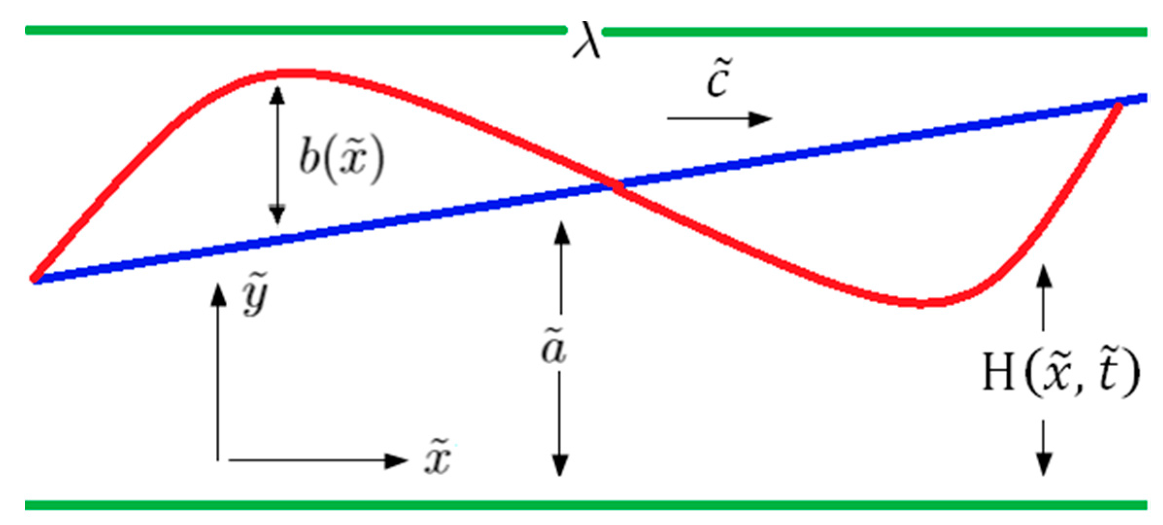
2. Mathematical Formulation

Let us consider the peristaltic blood-like flow of a viscous fluid, incompressible and electrically conducting nanofluid through a two dimensional non-uniform channel with peristaltic waves travelling down its walls. We have selected a Cartesian coordinate system for the channel in such a way that the x ˜ axis is taken along the axial direction and the y ˜ axis is taken along the transverse direction (see Figure 1). The geometry of the governing flow problem can be described as:
H ( x ˜ , t ˜ ) = b ( x ˜ ) + a ˜ sin 2 π λ ( x ˜ c ˜ t ˜ ) ,
where:
b ( x ˜ ) = b 0 + Κ ¯ x ˜ .
The governing equationw of continuity, motion, thermal energy and nanoparticle concentration for peristaltic nanofluid blood flow can be written as [17]:
u ˜ x ˜ + v ˜ y ˜ = 0 ,
ρ f ( u ˜ t ˜ + u ˜ u ˜ x ˜ + v ˜ u ˜ y ˜ ) = p ˜ x ˜ + μ ( S x ˜ x ˜ x ˜ + S x ˜ y ˜ y ˜ ) + g [ ( 1 F ) ρ f 0 ζ ( T T 0 ) ( ρ p ρ f 0 ) ( F F 0 ) ] ,
ρ f ( v ˜ t ˜ + u ˜ v ˜ x ˜ + v ˜ v ˜ y ˜ ) = p ˜ x ˜ + μ ( S y ˜ x ˜ x ˜ + S y ˜ y ˜ y ˜ ) + g [ ( 1 F ) ρ f 0 ζ ( T T 0 ) ( ρ p ρ f 0 ) ( F F 0 ) ] ,
( ρ c ) f ( T t ˜ + u ˜ T x ˜ + v ˜ T y ˜ ) = 𝒦 n f ( 2 T x ˜ 2 + 2 T y ˜ 2 ) + ( ρ c ) p D B ( F x ˜ T x ˜ + F y ˜ T y ˜ ) + D T T 0 ( ( T x ˜ ) 2 + ( T y ˜ ) 2 ) ,
( F t ˜ + u ˜ F x ˜ + v ˜ F y ˜ ) = D B ( 2 F x ˜ 2 + 2 F y ˜ 2 ) + D T T 0 ( 2 T x ˜ 2 + 2 T y ˜ 2 ) .
The stress tensor for the Jeffrey fluid is defined as [17]:
S = μ 1 + λ 1 ( γ ˙ + λ 2 γ ¨ ) .
Introducing the following non-dimensional quantities, we have:
x = x ¯ λ , y = y ¯ a ˜ , t = c ˜ t ˜ λ , u = u ˜ c ˜ , v = v ˜ c ˜ δ , p = a 2 p ˜ c ˜ λ μ , h = H a ˜ , ϕ = b o a ˜ , ν = μ ρ f o , Re = c ˜ ρ f a ˜ μ , θ = T T 0 T 1 T 0 , Φ = F F 0 F 1 F 0 , G r F = g a ˜ 3 ( F 1 F 0 ) ( ρ p ρ f 0 ) ρ f 0 ν 2 , N b = ( ρ c ) p D B ( F 1 F 0 ) K n f , δ = a ˜ λ , G r T = ζ g a ˜ 3 ( 1 F 0 ) ( T 1 T 0 ) ν 2 , N t = ( ρ c ) p D T ( T 1 T 0 ) K n f T 0 , S = a ˜ μ c ˜ S .
Let us consider the creeping flow under the assumptions of long wavelength and low Reynolds number approximation. Using Equation (9) in Equations (4)–(8) we get:
p x = 1 1 + λ 1 2 u y 2 + G r T θ G r F Φ ,
2 θ y 2 + N b θ y Φ y + N t ( θ y ) 2 = 0 ,
2 Φ y 2 + N t N b ( 2 θ y 2 )   = 0 ,
subject to no slip boundary conditions:
u y = θ ( y ) = Φ ( y ) = 0 ,  at  y = 0 ,
u ( y ) = 0 ,   θ ( y ) = Φ ( y ) = 1 ,  at  y = h = 1 + χ ,
where χ = k x λ b 0 + ϕ sin 2 π ( x t ) and ϕ   is the amplitude ratio. The expression for the compliant wall can be defined as:
L ( χ ) = p p 0 ,
where p 0 is pressure on outside surface of the wall due to tension in muscle, which is assumed to be zero here. The L operator is used to described the stretched membrane with viscosity damping force such as:
L = T 2 x 2 + M 2 t 2 + D t ,
p x = E 1 3 χ x 3 + E 2 3 χ t 2 x + E 3 2 χ t x = 1 1 + λ 1 2 u y 2 .
In the above equation, E 1 = T a ˜ 3 c ˜ λ 3 μ , E 2 = M a ˜ 3 c ˜ / λ 3 μ , E 3 = D a ˜ 3 / λ 2 μ are the non-dimensional elasticity quantities.

3. Entropy Generation

The volumetric rate of the local entropy generation of the nanofluid can be defined as [33]:
S g e n ' ' ' = K n f T 2 ( ( T x ˜ ) 2 + ( ( T y ˜ ) 2 ) ) + μ n f T ( 2 ( ( u ˜ x ˜ ) 2 + ( v ˜ y ˜ ) 2 ) + ( u ˜ y ˜ + v ˜ x ˜ ) 2 ) + R D B T ( T y ˜ ) ( C y ˜ ) + R D B F 0 ( F ) 2 .
The above equation represents entropy generation due to heat transfer, fluid friction irreversibility and combine product of concentration and temperature gradient. respectively. A characteristic entropy generation is given by [33]:
S G ' ' ' = K f ( T 1 T 0 ) 2 T 2 a ˜ 2 .
Using Equations (18) and (19), the dimensionless entropy generation number can be expressed as follows:
N S = S g e n ' ' ' S g ' ' ' = ( K n f K f ) ( ( θ y ) 2 ) + B r 1 Ω ( μ n f μ f ( 1 + λ 1 ) ) ( u y ) 2 + ε ( θ y ) ( Φ y ) + Γ ( Λ Ω ) 2 ( Φ y ) 2 ,
where   B r ,   Ω , ε , Γ  and  Λ are defined as:
B r = c ˜ 2 μ f K f ( T 1 T 0 ) , ε = R D B T K f ( F 1 F 0 T 1 T 0 ) , Ω = ( T 1 T 0 ) T , Γ = R D B F 0 K f , Λ = F 1 F 0 F 0 .
The nanofluid viscosity can be defined as [34]:
μ n f = μ f ( 1 ϕ ¯ ) 2.5 ,
where μ f is the viscosity of the base fluid, ϕ ¯ is the solid volume fraction which is valid for   0.01 ϕ ¯ 0.04 . When the thermal conductivity of the particle is over 100 times larger than that of base fluid, the thermal conductivity in the sense of macroscopic effective medium theory known as Maxwell model [34] which is given as:
K n f = κ p + 2 κ f + 2 ϕ ¯ ( κ p κ f ) κ p + 2 κ f ϕ ¯ ( κ p κ f ) κ f .
Here, κ p , κ f are the thermal conductivities of the nanoparticles and nanofluid, respectively.

4. Solution of the Problem

The solution of the non-linear coupled partial differential equations can be solve with the help of homotopy perturbation method [13]. The homotopy for Equations (10)–(12) can be written as:
h ¯ ( ω , q ) = ( 1 q ) ( 1 ( ω ) 1 ( ω ˇ 0 ) ) + q ( 1 ( ω ) + G r T Θ G r F ϑ C )   = 0 ,
h ¯ ( ϑ , q ) = ( 1 q ) ( 2 ( ϑ ) 2 ( ϑ ˇ 0 ) ) + q ( 2 ( ϑ ) + N b Θ y ϑ y + N t ( ϑ y ) 2 ) = 0 ,
h ¯ ( Θ , q ) = ( 1 q ) ( 2 ( Θ ) 2 ( Θ ˇ 0 ) ) + q ( 2 ( Θ ) + N t N b ( 2 ϑ y 2 ) ) = 0.
We have selected the following linear operator as:
1 = 1 1 + λ 1 2 y 2 ,
2 = 2 y 2 ,
and the initial guess is defined as:
ω ˇ 0 = ( y 2 h 2 ) ( 1 + λ 1 ) ,
Θ ˇ 0 = ϑ ˇ 0 = y h 1 .
The expansion series can be defined as:
ω ( x , y ) = ω 0 + q ω 1 + q 2 ω 2 + ,
ϑ ( x , y ) = ϑ 0 + q ϑ 1 + q 2 ϑ 2 + ,
Θ ( x , y ) = Θ 0 + q Θ 1 + q 2 Θ 2 + .
Using Equations (31)–(33) in Equations (24)–(26) and comparing the powers of q we get a system of linear differential equations with their relevant boundary conditions. According to the scheme of HPM, we obtained the solution as   q 1 , and we get:
u   ( x , y ) = ω ( x , y ) | q 1 = ω 0 + q ω 1 + q 2 ω 2 + ,
θ ( x , y ) = ϑ ( x , y ) | q 1 = ϑ 0 + q ϑ 1 + q 2 ϑ 2 + ,
Φ ( x , y ) = Θ ( x , y ) | q 1 = Θ 0 + q Θ 1 + q 2 Θ 2 + .
The solution of velocity profile, temperature profile and nanoparticle concentration are written in simplified form as:
u ( y ) = ( 1 + λ 1 ) ( ( 6 3 C G r F + G r T ) h 3 + 3 ( 2 + C ) h y 2 + ( G r F + G r T ) y 3 ) 6 h + G r T ( 1 + λ 1 ) ( N b + N t ) ( h 4 2 h y 3 + y 4 ) ( 24 h 2 ) + ( 1 + λ 1 ) N t ( N b + N t ) ( 15 G r F h 4 ( h 4 2 h y 3 + y 4 ) + G r T N b ( N b + N t ) ( 3 h 6 10 h 3 y 3 + 15 y 4 h 2 12 h y 5 12 h y 5 + 4 y 6 ) ) 360 h 6 N b ,
θ ( x , y ) = y h + ( h N b y + h N t y N b y 2 N t y 2 ) ( 2 h 2 )     + 1 2520 h 14 N t ( N b + N t ) 2 y ( h 7 ( 105 h 6 21 h 4 N b N t ( N b + N t )     + 20 N t 2 ( N b + N t ) 2 )     35 h 6 ( 9 h 6 3 h 4 N b N t ( N b + N t ) + 4 N t 2 ( N b + N t ) 2 ) y     + 140 h 5 ( 3 h 6 2 h 4 N b N t ( N b + N t ) + 4 N t 2 ( N b + N t ) 2 ) y 2     70 h 4 ( 3 h 6 6 h 4 N b N t ( N b + N t ) + 20 N t 2 ( N b + N t ) 2 ) y 3     + 112 h 3 N t ( N b + N t ) ( 3 h 4 N b + 20 N t ( N b + N t ) ) y 4     + 112 h 2 N t ( N b + N t ) ( h 4 N b 20 N t ( N b + N t ) ) y 5     + 1280 h N t 2 ( N b + N t ) 2 y 6 320 N t 2 ( N b + N t ) 2 y 7 ) ,
Φ ( x , y ) = y h + ( h N b N t y h N t 2 y + N b N t y 2 + N t 2 y ) ( 2 h 2 N b ) + N t 2 ( N b + N t ) 2 y ( 2 h 4 + 5 h 2 y 2 5 h y 3 + 2 y 4 ) 30 h 6 N b ,
where:
C = ( E 1 + E 2 ) ( 8 π 3 ϕ cos [ 2 π ( x t ) ] ) + 4 E 3 π 2 ϕ sin [ 2 π ( x t ) ] .

5. Numerical Results and Discussion

In this section the influence of some controlling parameters such as Brownian motion parameter N b , thermophoresis parameter N t , non dimensional elasticity parameters E 1 ,   E 2 and E 3 , basic density Grashof number G r F , thermal Grashof number G r T , Brinkman group parameter B Ω 1 and dimensionless constant parameter on temperature profile, concentration profile, entropy generation and velocity profile are presented graphically. Furthermore, In Equation (10), by taking λ 1 = 0 ,   G r T = G r F = 0 ,   the present results can be reduced to the results obtained by Shapiro et al. [35] and Srivastava [36] for a Newtonian fluid case ( Power Law index  n = 1 ) . Moreover, Equation (10) can also reduces to the same result obtained by Gupta and Seshadri [37] by taking λ 1 = 0 ,   G r T = G r F = 0 . The present analysis can also be reduced to the similar results obtained by Mekheimer [18] for Newtonian fluids ( couple stres parameter  γ ) by taking λ 1 = 0 ,   G r T = G r F = 0.   Table 1 shows the numerical comparison for velocity profile between a Newtonian and a non-Newtonian fluid.
Figure 2 depicts the effect of Brownian motion N b and thermophoresis parameter N t on temperature profile. It shows that temperature increases for the higher values of N b   and N t indicating that the boundary layer is increasingly heated and there is progressive thickening in the thermal boundary layer. The reason behind is that Brownian motion enhances the thermal conductivity of a nanofluid by generating micro-mixing and as a consequence of which the temperature profile increases strongly. Also it is manifest from Equations (11) and (12) that the temperature is directly proportional to   N t   which further tells us that the temperature profile will increase for the higher values of N t . Such results have significant importance in the case of electromagnetic hyperthermia treatment because the vital purpose of electromagnetic hyperthermia is to rise the temperature of cancerous tissues above 42 °C. We observe in Figure 3 that the concentration profile is consistently reduced with an increasing N b while enhanced thermophoresis clearly corresponds to a significant increase in Φ ( y ) , i.e. with an increment in Brownian motion, the impact of thermal conductivity increases and thus, the concentration profile decreases.
The behavior of entropy generation for some pertinent parameters such as nondimensional elasticity parameters E 1 ,   E 2 , E 3 , Brownian motion parameter N b , thermophoresis parameter   N t , Basic density Grashof number G r F , thermal Grashof number G r T and dimensionless constant parameter are plotted in Figure 4, Figure 5, Figure 6, Figure 7 and Figure 8a. Figure 4 shows a strong deceleration in entropy generation for greater values of E 1 and E 2 . An increase in tension or stiffness in the channel walls lead to decrease in temperature and consequently entropy generation reduces. Figure 5 reveals that entropy generation is an accelerating function for E 3 and B r Ω 1 . The Brinkman group parameter B Ω 1 regulates significance of viscous effects and it is also noticed that this parameter is associated with nanofluid viscosity term, i.e., B r 1 Ω ( μ n f μ f ) ( u y ) 2 in Equation (18). The Brinkman group parameter appears directly proportional to the square of the velocity and an increase in B Ω 1 evidently accelerates flow and as a result entropy will increase. The behavior of N S for different values of N t and N b is demonstrated in Figure 6. From both figures, it is clear that entropy generation increases for higher values of N t and N b . Physical interpretation of this behavior is that with the increase in the Brownian motion parameter and thermophoresis parameter the process of heat generation and heat transfer increases, i.e. N t and N b serve to boost the entropy generation markedly. Figure 7 provides a perspective of the influence of G r T and   G r F on N S ( y ) . Inspection of these graphs reveals that entropy generation is an increasing function with the increase in G r T and   G r F . Entropy generation is reduced strongly, as seen in Figure 8a for higher values of . However, beyond a certain point negligible entropy effect is observed. Velocity profiles are displayed in Figure 8b and Figure 9 for various values of E 1 , E 2 and E 3 . In such cases the flow is decelerating for progressive values of   E 1 , E 2 and E 3 . Due to the increase in E 1 and E 2 less resistance is offered to the flow and velocity distribution decreases similarly, E 3 represents the damping effect which creates resistivity in the flow and velocity profile decreases with the enhance in E 3 . Physically, larger values in E 1 reduces tension in the walls of blood vessels which speeds up the blood flow. The walls of the channel or blood vessels are under strong influence of damping for higher values of E 3 . In such situations the vessels or arteries are required the higher amount of force to extent and taken up the blood ejected from the heart.

6. Conclusions

Entropy generation during peristaltic blood-like flow of a non-Newtonian nanofluid in a channel having complaint walls has been studied in this article. The governing flow problem is solved under the approximations of long wave length and zeros Reynolds number. The resulting non-linear coupled differential equations are solved by means of the homotopy perturbation method and the solutions have been obtained up to 3rd order approximation. Numerical solutions have been obtained with the help of the computational software “Mathematica” to calculate the expression for velocity profile, temperature profile and concentration profile. The main outcomes of the present investigation are categorized below:
  • Temperature distribution increases when N b and N t increases.
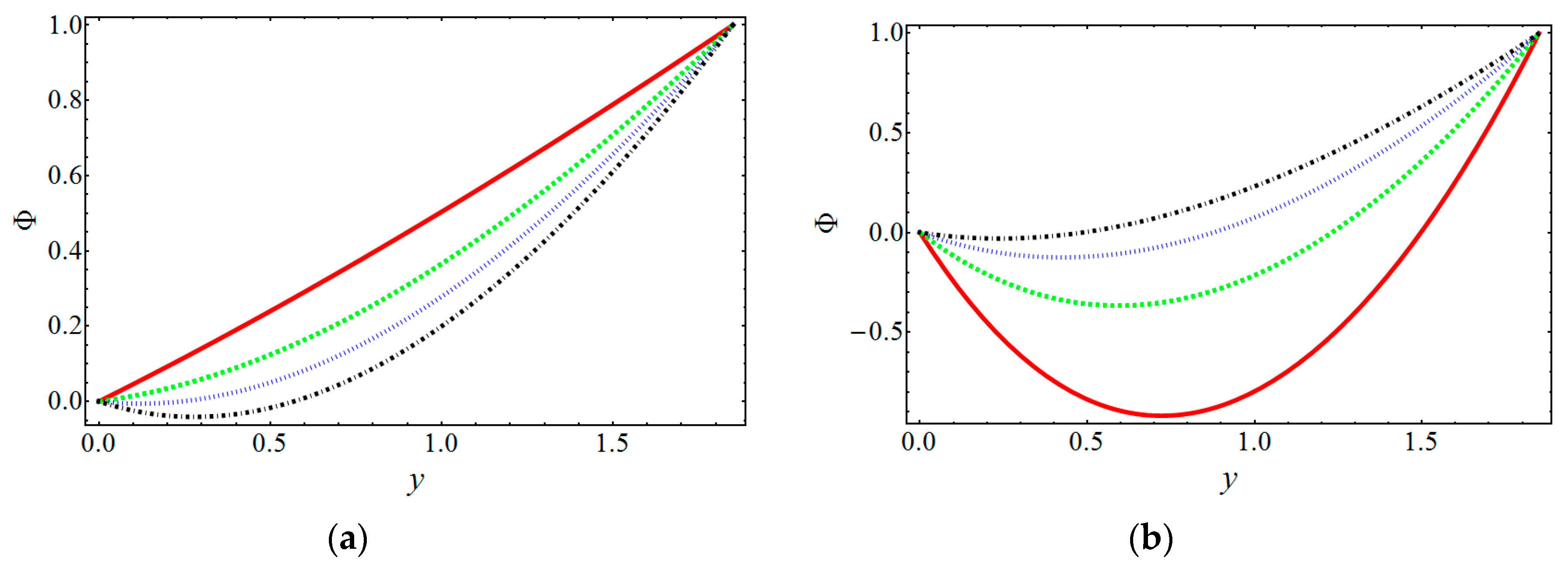
  • Concentration distribution is increasing for N b but its attitude is opposite for N t .
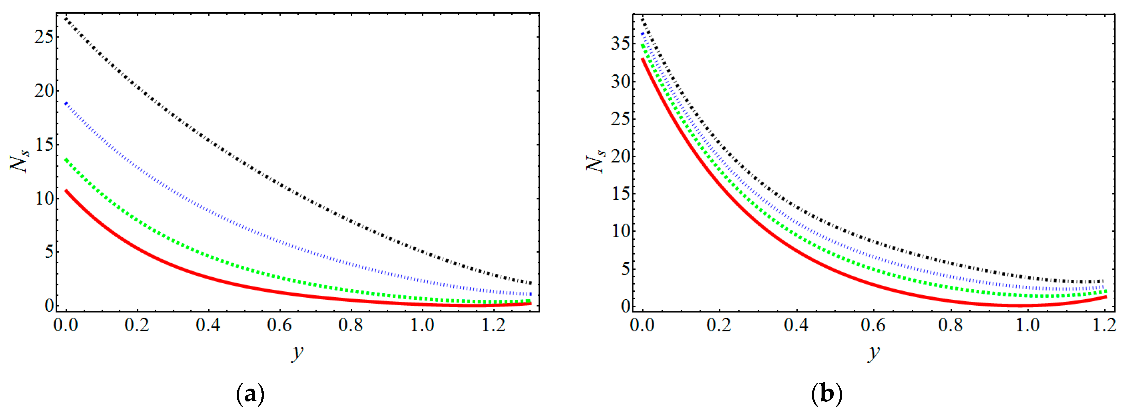
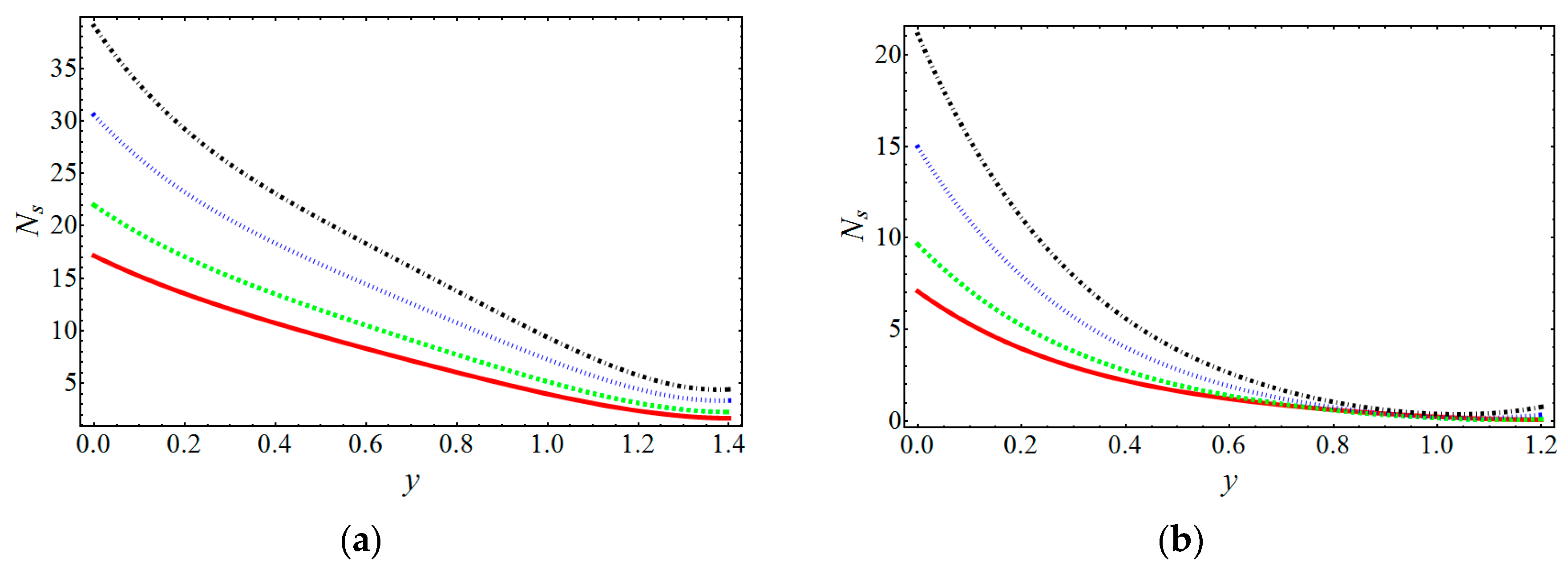
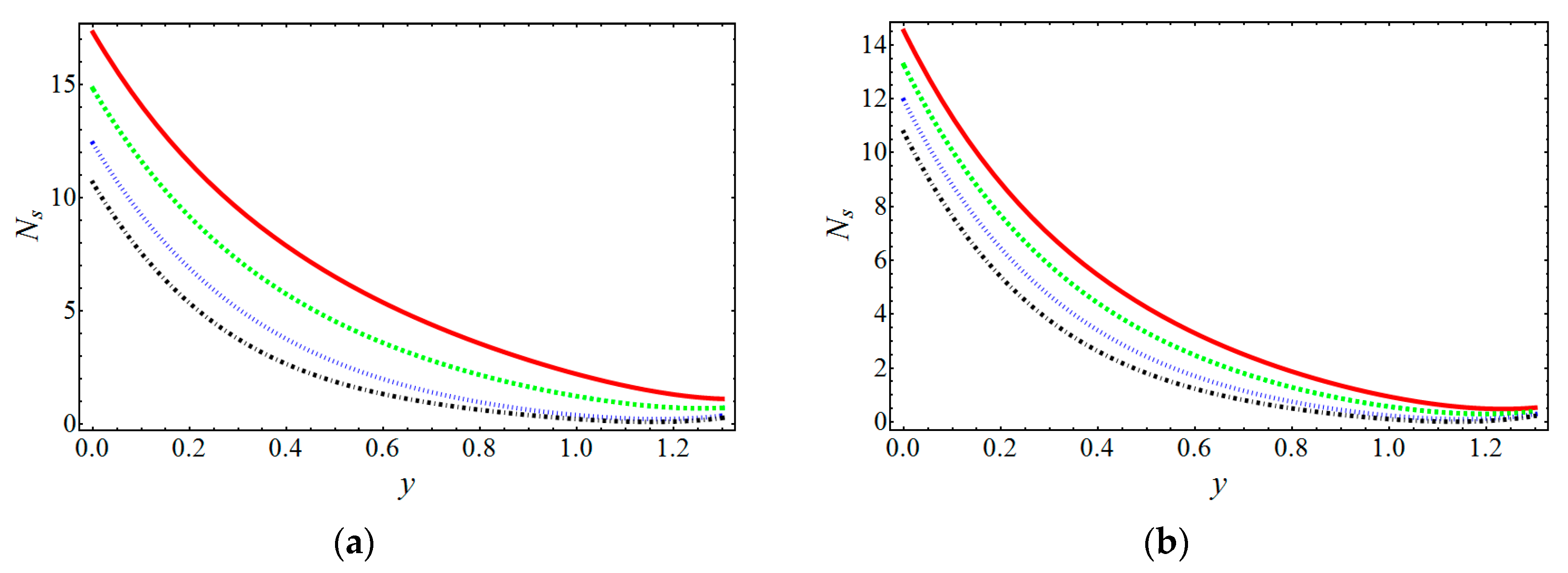
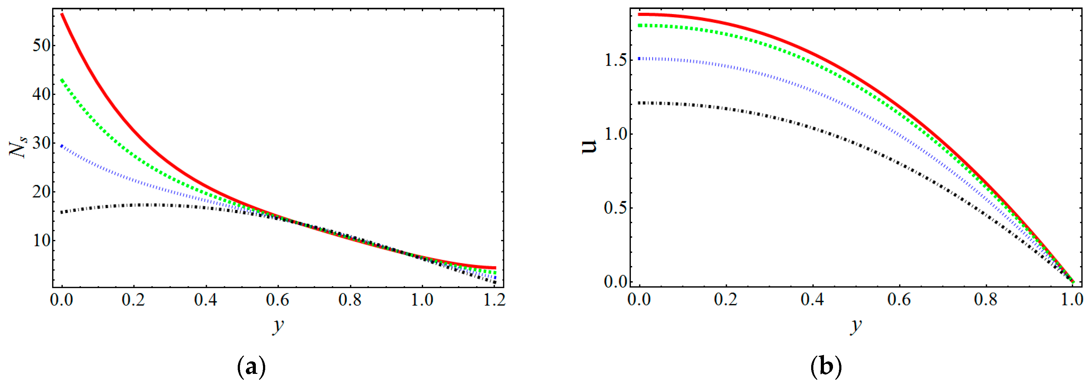
  • Entropy generation is increasing for different values of E 3 , B Ω 1 ,   N t and N b but it is a decreasing function for the parameters G r T ,   G r F ,   and E 1 .
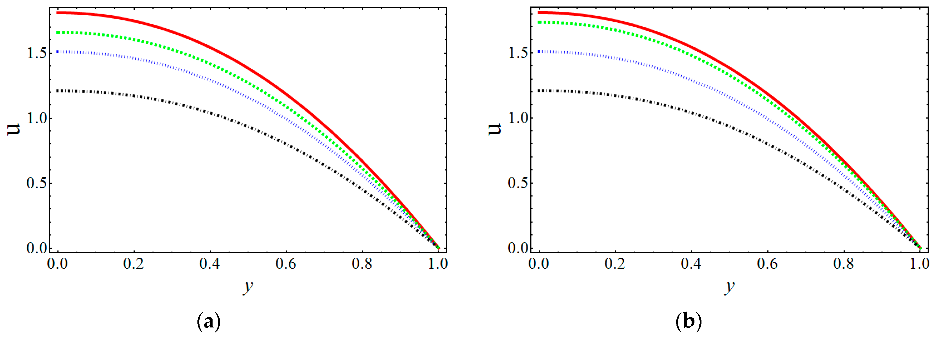
  • Velocity profile diminishes for large values of E 1 ,   E 2   and E 3 .
  • The present model may be beneficial in understanding the dynamic of blood flow small blood vessels by taking into account the important wall elastic parameters.

Acknowledgments

Project supported by the National Natural Science foundation of China (No. 11371242).

Author Contributions

Mohammad Mehdi Rashidi and Munawwar Ali Abbas conceived and desgined the mathematical formulation of the problem, whereas solution of the problem and graphical results is analyzed by Yanqin Bai and Muhammad Mubashir Bhatti. All authors have read and approved the final manuscript.

Conflicts of Interest

The authors declare no conflict of interest.

Nomenclature

u ˜ ,   v ˜ velocity components ( m / s )
x ˜ ,   y ˜ Cartesian coordinate ( m )
p ˜ pressure in fixed frame ( N / m 2 )
a ˜ wave amplitude ( m )
b ( x ˜ ) width of the channel
b 0 half width at the inlet
c ˜ wave velocity ( m / s )
N s dimensionless entropy number
Re Reynolds number
t ˜ time ( s )
G r F basic density Grashof number
G r T thermal Grashof number
N b Brownian motion parameter
N t thermophoresis parameter
Κ ¯ ( 1 ) constant
  B r Brinkman number
T environmental temperature (K)
Λ constant parameter
M wall mass per unit area
D coefficient of viscous damping
T ,   F temperature ( K ) and concentration
g acceleration due to gravity ( m / s 2 )
D B Brownian diffusion coefficient ( m 2 / s )
D T thermophoretic diffusion coefficient ( m 2 / s )
K mean absorption constant
S stress tensor

Greek Symbols

κ p thermal conductivities of the nano particles
λ 1 ratio b/w relaxation to retardation time
K n f thermal conductivity of nanofluid ( W / m K )
μ viscosity of the fluid ( N s / m 2 )
Γ diffusive coefficient
ε dimensionless constant parameter
Ω dimensionless temperature difference
Φ nano particle volume fraction
θ temperature profile
δ wave number ( m 1 )
γ ˙ shear rate
c p effective heat capacity of nano particle ( J / K )
ν nanofluid kinematic viscosity ( m 2 / s )
( ρ ) p nano particle mass density ( kg / m 3 )
ρ f fluid density ( kg / m 3 )
ρ f 0 fluid density at the reference temperature ( T 0 ) ( kg / m 3 )
ζ volumetric expansion coefficient of the fluid
( ρ c ) f heat capacity of fluid ( J / K )
λ wavelength ( m )
ϕ amplitude ratio
λ 2 delay time

References

  1. Villone, M.M.; Greco, F.; Hulsen, M.A.; Maffettone, P.L. Simulation of an elastic particle in Newtonian and Viscoelastic fluids subjected to confined shear flow. J. Non-Newton. Fluid Mech. 2014, 210, 47–55. [Google Scholar] [CrossRef]
  2. Bae, H.-O. Regularity criterion for generalized Newtonian fluids in bounded domains. J. Math. Anal. Appl. 2015, 421, 489–500. [Google Scholar] [CrossRef]
  3. Hatami, M.; Domairry, G. Transient vertically motion of a soluble particle in a Newtonian fluid media. Powder Technol. 2014, 253, 481–485. [Google Scholar] [CrossRef]
  4. Rashidi, M.M.; Rastegari, M.T.; Asadi, M.; Bég, O.A. A study of non-Newtonian flow and heat transfer over a non-isothermal wedge using the homotopy analysis method. Chem. Eng. Commun. 2012, 199, 231–256. [Google Scholar] [CrossRef]
  5. Nadeem, S.; Akbar, N.S.; Hendi, A.A.; Hayat, T. Power law fluid model for blood flow through a tapered artery with a stenosis. Appl. Math. Comput. 2011, 217, 7108–7116. [Google Scholar] [CrossRef]
  6. Ashorynejad, H.R.; Javaherdeh, K.; Sheikholeslami, M.; Ganji, D.D. Investigation of the heat transfer of a non-Newtonian fluid flow in an axisymmetric channel with porous wall using Parameterized Perturbation Method (PPM). J. Frankl. Inst. 2014, 351, 701–712. [Google Scholar] [CrossRef]
  7. Choi, S.U.S. Enhancing thermal conductivity of fluids with nanoparticles. In Proceedings of ASME International Mechanical Engineering Congress & Exposition, San Francisco, CA, USA, 12–17 November 1995.
  8. Freidoonimehr, N.; Rashidi, M.M. Dual Solutions for MHD Jeffery–Hamel Nano-fluid Flow in Non-parallel Walls using Predictor Homotopy Analysis Dual Solutions Method. J. Appl. Fluid Mech. 2015, 8, 911–919. [Google Scholar]
  9. Sheikholeslami, M.; Gorji-Bandpy, M.; Ganji, D.D.; Soleimani, S. MHD natural convection in a nanofluid filled inclined enclosure with sinusoidal wall using CVFEM. Neural Comput. Appl. 2014, 24, 873–882. [Google Scholar] [CrossRef]
  10. Freidoonimehr, N.; Rashidi, M.M.; Mahmud, S. Unsteady MHD free convective flow past a permeable stretching vertical surface in a nano-fluid. Int. J. Therm. Sci. 2015, 87, 136–145. [Google Scholar] [CrossRef]
  11. Akbar, N.S.; Rahman, S.U.; Ellahi, R.; Nadeem, S. Nano fluid flow in tapering stenosed arteries with permeable walls. Int. J. Therm. Sci. 2014, 85, 54–61. [Google Scholar] [CrossRef]
  12. Freidoonimehr, N.; Rostami, B.; Rashidi, M.M.; Momoniat, E. Analytical Modelling of Three-Dimensional Squeezing Nanofluid Flow in a Rotating Channel on a Lower Stretching Porous Wall. Math. Probl. Eng. 2014. [Google Scholar] [CrossRef]
  13. Abbas, M.A.; Bai, Y.; Bhatti, M.M.; Rashidi, M.M. Three dimensional peristaltic flow of hyperbolic tangent fluid in non-uniform channel having flexible walls. Alex. Eng. J. 2015, in press. [Google Scholar] [CrossRef]
  14. Mekheimer, K.S. Peristaltic flow of a couple stress fluid in an annulus: Application of an endoscope. Physica A 2008, 387, 2403–2415. [Google Scholar] [CrossRef]
  15. Akbar, N.S.; Nadeem, S.; Mekheimer, K.S. Rheological properties of Reiner-Rivlin fluid model for blood flow through tapered artery with stenosis. J. Egypt. Math. Soc. 2016, 24, 138–142. [Google Scholar] [CrossRef]
  16. Sinha, A.; Shit, G.C.; Ranjit, N.K. Peristaltic transport of MHD flow and heat transfer in an asymmetric channel: Effects of variable viscosity, velocity-slip and temperature jump. Alex. Eng. J. 2015, 54, 691–704. [Google Scholar] [CrossRef]
  17. Abbas, M.A.; Bai, Y.; Rashidi, M.M.; Bhatti, M.M. Application of drug delivery in megnetohydrodynamics peristaltic blood flow of nano fluid in a nan-uniform channel. J. Mech. Med. Biol. 2015. [Google Scholar] [CrossRef]
  18. Mekheimer, K.S. Peristaltic flow of blood under effect of a magnetic field in a non-uniform channels. Appl. Math. Comput. 2004, 153, 763–777. [Google Scholar] [CrossRef]
  19. Bég, O.A.; Keimanesh, M.; Rashidi, M.M.; Davoodi, M.; Branch, S.T. Multi-Step dtm simulation of magneto-peristaltic flow of a conducting Williamson viscoelastic fluid. Int. J. Appl. Math. Mech. 2013, 9, 1–24. [Google Scholar]
  20. Bejan, A. Second law analysis in heat transfer. Energy 1980, 5, 720–732. [Google Scholar] [CrossRef]
  21. Bejan, A. Entropy Generation Minimization: The Method of Thermodynamic Optimization of Finite-Time Systems and Finite-Time Processes; CRC Press: New York, NY, USA, 1996. [Google Scholar]
  22. Revellin, R.; Lips, S.; Khandekar, S.; Bonjour, J. Local entropy generation for saturated two-phase flow. Energy 2009, 34, 1113–1121. [Google Scholar] [CrossRef]
  23. Salas, H.; Cuevas, S.; de Haro, M.L. Entropy generation analysis of magnetohydrodynamic induction devices. J. Phys. D Appl. Phys. 1999, 32. [Google Scholar] [CrossRef]
  24. Akbar, N.S. Entropy Generation Analysis for a CNT Suspension Nanofluid in Plumb Ducts with Peristalsis. Entropy 2015, 17, 1411–1424. [Google Scholar] [CrossRef]
  25. Akbar, N.S. Entropy generation and energy conversion rate for the peristaltic flow in a tube with magnetic field. Energy 2015, 82, 23–30. [Google Scholar] [CrossRef]
  26. Rashidi, M.M.; Abelman, S.; Mehr, N.F. Entropy generation in steady MHD flow due to a rotating porous disk in a nanofluid. Int. J. Heat Mass Transf. 2013, 62, 515–525. [Google Scholar] [CrossRef]
  27. Rashidi, M.M.; Bagheri, S.; Momoniat, E.; Freidoonimehr, N. Entropy analysis of convective MHD flow of third grade non-Newtonian fluid over a stretching sheet. Ain Shams Eng. J. 2015, in press. [Google Scholar] [CrossRef]
  28. Lee, M.Y.; Kim, H.J. Heat Transfer Characteristics of a Speaker Using Nano-Sized Ferrofluid. Entropy 2014, 16, 5891–5900. [Google Scholar] [CrossRef]
  29. Humeau-Heurtier, A.; Baumert, M.; Mahé, G.; Abraham, P. Multiscale Compression Entropy of Microvascular Blood Flow Signals: Comparison of Results from Laser Speckle Contrastand Laser Doppler Flowmetry Data in Healthy Subjects. Entropy 2014, 16, 5777–5795. [Google Scholar] [CrossRef] [Green Version]
  30. Galanis, N.; Rashidi, M.M. Entropy generation in non-Newtonian fluids due to heat and mass transfer in the entrance region of ducts. Heat Mass Transf. 2012, 48, 1647–1662. [Google Scholar] [CrossRef]
  31. Hassan, M.; Sadri, R.; Ahmadi, G.; Dahari, M.B.; Kazi, S.N.; Safaei, M.R.; Sadeghinezhad, E. Numerical study of entropy generation in a flowing nanofluid used in micro-and minichannels. Entropy 2013, 15, 144–155. [Google Scholar] [CrossRef]
  32. Sheikholeslami, M.; Ganji, D.D. Entropy generation of nanofluid in presence of magnetic field using Lattice Boltzmann Method. Physica A 2015, 417, 273–286. [Google Scholar] [CrossRef]
  33. Baag, S.; Mishra, S.R.; Dash, G.C.; Acharya, M.R. Entropy generation analysis for viscoelastic MHD flow over a stretching sheet embedded in a porous medium. Ain Shams Eng. J. 2016, in press. [Google Scholar] [CrossRef]
  34. Mahian, O.; Kianifar, A.; Kleinstreuer, C.; Al-Nimr, M.M.; Pop, I.; Sahin, A.Z.; Wongwises, S. A review of entropy generation in nanofluid flow. Int. J. Heat Mass Transf. 2013, 65, 514–532. [Google Scholar] [CrossRef]
  35. Shapiro, A.H.; Jaffrin, M.Y.; Weinberg, S.L. Peristaltic pumping with long wavelength at low Reynolds number. J. Fluid Mech. 1969, 37, 799–825. [Google Scholar] [CrossRef]
  36. Srivastava, L.M.; Srivastava, V.P. Peristaltic transport of a power-law fluid: Application to the ductus efferentes of the reproductive tract. Rheol. Acta. 1988, 27, 428–433. [Google Scholar] [CrossRef]
  37. Gupta, B.B.; Seshadri, V. Peristaltic pumping in non-uniform tubes. J. Biomech. 1976, 9, 105–109. [Google Scholar] [CrossRef]
Figure 1. Geometry of the problem.
Entropy 18 00090 g001
Figure 2. Temperature distribution for various values of N t and N b . (a) red line: N b = 0.1 , green line: N b = 0.3 , blue line: N b = 0.6 , black line: N b = 0.9 ; (b) red line: N t = 0.1 , green line: N t = 0.3 , blue line: N t = 0.6 , black line: N t = 0.9 .
Entropy 18 00090 g002
Figure 3. Concentration distribution for various values of N b and N t . (a) red line: N b = 0.1 , green line:   N b = 0.3 , blue line: N b = 0.6 , black line: N b = 0.9 ; (b) red line: N t = 0.1 , green line: N t = 0.3 , blue line: N t = 0.6 , black line: N t = 0.9 .
Entropy 18 00090 g003
Figure 4. Entropy generation for various values of E 1 and E 2 . (a) red line: E 1 = 0.1 , green line: E 1 = 0.3 , blue line: E 1 = 0.6 , black line: E 1 = 0.9 ; (b) red line: E 2 = 0.1 , green line: E 2 = 0.3 , blue line: E 2 = 0.6 , black line: E 2 = 0.9 .
Entropy 18 00090 g004
Figure 5. Entropy generation for various values of E 3 and B Ω 1 . (a) red line: E 3 = 0.1 , green line: E 3 = 0.3 , blue line:   E 3 = 0.6 , black line: E 3 = 0.9 ; (b) red line: B Ω 1 = 0.1 , green line: B Ω 1 = 0.3 , blue line: B Ω 1 = 0.6 , black line: B Ω 1 = 0.9 .
Entropy 18 00090 g005
Figure 6. Entropy generation for various values of N t and N b . (a) red line: N t = 0.1 , green line: N t = 0.3 , blue line: N t = 0.6 , black line: N t = 0.9 ; (b) red line: N b = 0.1 , green line: N b = 0.3 , blue line: N b = 0.6 , black line: N b = 0.9 .
Entropy 18 00090 g006
Figure 7. Entropy generation for various values of G r T and   G r F . (a) red line: G r T = 0.1 , green line: G r T = 0.3 , blue line: G r T = 0.6 , black line: G r T = 0.9 ; (b) red line: G r F = 0.1 , green line: G r F = 0.3 , blue line: G r F = 0.6 , black line: G r F = 0.9 .
Entropy 18 00090 g007
Figure 8. (a) Entropy generation for various values of . Red line: ε = 0.01 , green line: ε = 0.03 , blue line: ε = 0.06 , black line: ε = 0.09 ; (b) Velocity profile for various values of E 1 . Red line: E 1 = 0.1 , green line: E 1 = 0.3 , blue line: E 1 = 0.6 , black line: E 1 = 0.9 .
Entropy 18 00090 g008
Figure 9. Velocity profile for various values of E 2 and E 3 . (a) red line: E 2 = 0.1 , green line: E 2 = 0.3 , blue line: E 2 = 0.6 , black line: E 2 = 0.9 ; (b) red line: E 3 = 0.1 , green line: E 3 = 0.3 , blue line: E 3 = 0.6 , black line: E 3 = 0.9 .
Entropy 18 00090 g009
Table 1. Numerical comparison of velocity profile between Newtonian and non-Newtonian fluids.
h(x,t)u(y)u(y)u(y)u(y)
λ 1   =   0 (Newtonian Fluid) λ 1   =   0.5 (Non-Newtonian Fluid) λ 1   = 0.8 (Non-Newtonian Fluid) λ 1 =   1.3 (Non-Newtonian Fluid)
0 0.5636 0.8454 1.0145 1.2964
0.1324 0.5584 0.8377 1.0052 1.2845
0.2649 0.5425 0.8137 0.9765 1.2477
0.3973 0.5150 0.7726 0.9271 1.1847
0.5298 0.4758 0.7138 0.8566 1.0945
0.6623 0.4247 0.6371 0.7645 0.9769
0.7947 0.3617 0.5426 0.6511 0.8320
0.9272 0.2871 0.4307 0.5169 0.6605
1.0596 0.2015 0.3022 0.3627 0.4634
1.1921 0.1054 0.1582 0.1898 0.2425
1.3246 0 0 0 0

