Constrained Inference When the Sampled and Target Populations Differ

Abstract

In the analysis of contingency tables, often one faces two difficult criteria: sampled and target populations are not identical and prior information translates to the presence of general linear inequality restrictions. Under these situations, we present new models of estimating cell probabilities related to four well-known methods of estimation. We prove that each model yields maximum likelihood estimators under those restrictions. The performance ranking of these methods under equality restrictions is known. We compare these methods under inequality restrictions in a simulation study. It reveals that these methods may rank differently under inequality restriction than with equality. These four methods are also compared while US census data are analyzed.

1. Introduction

When working with a sample contingency table, a researcher might need to adjust it based on information available from other sources. This information might come from prior surveys, censuses, established theories or other sources. Often it comes as marginal information such as row and/or column totals. For example, consider a data set where each subject is cross-classified by income (low/high) and urbanity (urban/rural), and, marginal information about income and urbanity is available from a census. One would like to adjust the sample data to conform to the desired margins from census.

For two-way contingency tables of size ($I\times J$), four well-known [1,2] margin-adjusting methods for estimating cell probabilities are raking (RAKE), least squares (LSQ), minimum chi-squared (MCSQ) and maximum likelihood under random sampling (MLRS). Assume that a random sample $\{n_{ij},1\le i\le I,1\le j\le J\}$ is available from a multinomial $(n,\mathit{\pi })$ probability distribution, where $n={\sum }_{i,j}{n}_{ij},\mathit{\pi }=({\pi }_{ij},\forall i,j)$. Let $p_{ij}=\frac{n_{ij}}{n}$ denote the sample cell proportions. Then RAKE finds the estimates $\{{\widehat{\pi }}_{ij}^{RK}\}$ that minimize the discrimination information,

$$\sum _{i=1}^I\sum _{j=1}^J{\widehat{\pi }}_{ij}ln(\frac{{\widehat{\pi }}_{ij}}{p_{ij}}),$$

under the marginal constraints

$$\sum _j{\widehat{\pi }}_{ij}={\pi }_{i+},\sum _i{\widehat{\pi }}_{ij}={\pi }_{+j},i=1,\dots ,I,j=1,\dots ,J,$$

(1)

where ${\widehat{\pi }}_{ij}$ denotes the estimators of target cell probabilities ${\pi }_{ij}$, $\forall i,j$, ${\pi }_{i+},{\pi }_{+j}$ are known, $\forall i,j$.

Under the same constraints (1), the methods LSQ, MCSQ, MLRS find the estimates $\{{\widehat{\pi }}_{ij}^{LSQ}\},\{{\widehat{\pi }}_{ij}^{MCSQ}\},\{{\widehat{\pi }}_{ij}^{ML}\}$ that minimize

$$\sum _{i=1}^I\sum _{j=1}^J\frac{{(p_{ij}-{\widehat{\pi }}_{ij})}^2}{p_{ij}},\sum _{i=1}^I\sum _{j=1}^J\frac{{({\widehat{\pi }}_{ij}-p_{ij})}^2}{{\widehat{\pi }}_{ij}},-\sum _{i=1}^I\sum _{j=1}^J{p}_{ij}ln\left({\widehat{\pi }}_{ij}\right),$$

respectively.

Instead of given marginal totals, one might like to use restrictions of a more general nature. Consider the survey data [3] from the second National Health and Nutrition Examination Survey (NHANES II).

Table 1. (a) Probability of income × urbanity and (b) probability of education × urbanity from NHANES II and the census.

NHANES II Data						1980 census
Income	Urban	Rural				Income	Urban	Rural
Low	0.3305	0.1955	0.5260			Low	0.2064	0.1127	0.3191
High	0.3200	0.1540	0.4740			High	0.4969	0.1840	0.6809
	0.6505	0.3495	1.0				0.7033	0.2967	1.0
(n = 16,547)						(n = 50,644,862)
					(a)
Education	Urban	Rural				Education	Urban	Rural
Low	0.4135	0.2682	0.6817			Low	0.4584	0.2107	0.6691
High	0.2360	0.0823	0.3183			High	0.2625	0.0684	0.3309
	0.6495	0.3505	1.0				0.7209	0.2791	1.0
(n = 8962)						(n = 114,290,384)
					(b)

a shows the sample proportions and corresponding census proportions of $2\times 2$ contingency tables of income by urbanity, and Table 1b shows the sample proportions and corresponding census proportions of $2\times 2$ contingency tables of education by urbanity. We observe differences in the census and sample values, possibly due to differences in target and sampled populations. For example, in Table 1a census data, the magnitude of row totals ($0.3191<0.6809$) is different from that of the sample data ($0.5260>0.4740$). Similarly, in Table 1b census data, the off-diagonal entries satisfy an order relation ($0.2625>0.2107$), but, in samples, the relation goes in the opposite direction ($0.2360<0.2682$). If such constraints are known a priori (e.g., from census or other sources), then it is wiser to incorporate them into the analysis while adjusting the sample data.

Much prior work (e.g., [2]) assumed that random samples were directly taken from the $\mathit{target\; population}$ with $\mathit{known}$ row and column margins (${\pi }_{i+},{\pi }_{+j}$ respectively). However, in practice, there are situations in which a random sample from the target population is inaccessible. For example, often sample units are too expensive to locate or unwilling to participate in the survey. In this case, to estimate the target cell probabilities, we have to take a random sample from a $\mathit{sampled\; population}$ that is systematically different from the target population. Clearly, the resulting estimators are typically biased. Researchers in [3] have studied such discrepancies under marginal row and column constraints. A similar problem in a regression context can be found in [4].

It is well-known that all four margin-adjusting methods are asymptotically equivalent under simple random sampling. However, their small sample results can be different. Using simulation methods, [5] found that MCSQ is best, followed by MLRS, RAKE and LSQ, in order of performance in average root mean squared error. However, for margin adjusting, [3] found that both RAKE and MLRS dominate MCSQ; and LSQ is inferior to all three methods when the sampled population is systematically different from the target population. In this paper, we consider general linear constraints (not necessarily marginal) under inequality restrictions and study the performance of those four methods. For simulation (Section 4), we have restricted our attention to $(2\times 2)$ tables to facilitate comparison with Little and Wu [3].

2. Solutions from Each Method

First, we vectorize the $I\times J$ contingency table of probabilities lexicographically, say, $\mathit{\pi }=\left({\pi }_{ij}\right)$ denote the $IJ\times 1$ target population probability vector. Thus, the pair $(i,j)=t$, for some $t,1\le t\le IJ$. We assume that the available knowledge of the population can be expressed as r constraints as

$${\mathit{A}}^T\mathit{\pi }\le \mathit{c},$$

(2)

where $\mathit{A}=\left(a_{ij}\right)$ denotes an $(IJ\times r),r\le I+J-1$, matrix of constants with rank$\left(\mathit{A}\right)=r$, $\mathit{c}=\left(c_i\right)$ denotes the $(r\times 1)$ corresponding known values vector.

First, we set each of these four methods as an optimization problem. The objective function $f\left(\mathit{\pi }\right)$ takes the form ${\sum }_{t=1}^{IJ}{\pi }_{t}ln\left(\frac{{\pi }_t}{p_t}\right)$ for RAKE, ${\sum }_{t=1}^{IJ}\frac{{({\pi }_t-p_t)}^2}{p_t}$ for LSQ, ${\sum }_{t=1}^{IJ}\frac{{({\pi }_t-p_t)}^2}{{\pi }_t}$ for MCSQ and $-{\sum }_{t=1}^{IJ}{p}_{t}ln{\pi }_t$ for MLRS, respectively. We seek to minimize the convex function $f\left(\mathit{\pi }\right)$ over a region ℓ defined as

$$\mathit{\ell }=\{\mathit{\pi }\mid {\mathit{A}}^T\mathit{\pi }\le \mathit{c},{\pi }_t>0,\forall t,\sum _t{\pi }_t=1\},$$

(3)

and this is known as the $\mathit{primal}$ problem. The Kuhn–Tucker method [6] identifies an equivalent $\mathit{dual}$ problem that could be substantially easier to solve than the primal problem (for larger $I,J$).

The $\mathit{Lagrangian}$ of the problem is defined by

$$L(\mathit{\lambda },\mathit{\pi })=f\left(\mathit{\pi }\right)+{\mathit{\lambda }}^T({\mathit{A}}^T\mathit{\pi }-\mathit{c}), \mathrm{i}\mathrm{f} {\lambda }_i\ge 0\mathrm{f}\mathrm{o}\mathrm{r} \mathrm{a}\mathrm{l}\mathrm{l} \mathit{i},\mathit{\pi }\in \mathit{\ell },$$

and, $L(\mathit{\lambda },\mathit{\pi })=-\infty ,$ if ${\lambda }_i<0$ for some $i,\mathit{\pi }\in \mathit{\ell },$ $L(\mathit{\lambda },\mathit{\pi })=+\infty ,$ if $\mathit{\pi }\notin \mathit{\ell }$, where $\mathit{\lambda }=({\lambda }_1,\dots ,{\lambda }_r)$ are called Lagrange multipliers.

Consider maximization in $\mathit{\lambda }$ and minimization in $\mathit{\pi }$ of $L(\mathit{\lambda },\mathit{\pi })$. Suppose there exists $({\mathit{\lambda }}^{*},{\mathit{\pi }}^{*})$ for which $L(\mathit{\lambda },{\mathit{\pi }}^{*})\le L({\mathit{\lambda }}^{*},{\mathit{\pi }}^{*})\le L({\mathit{\lambda }}^{*},\mathit{\pi }),\forall \mathit{\lambda },\mathit{\pi },$ if and only if

$$\begin{array}{c}\frac{\partial L}{\partial {\pi }_t}=\sum _s\mathrm{[}\frac{\partial f\left({\pi }_s\right)}{\partial {\pi }_s}+\sum _{i=1}^r{\lambda }_i(a_{it}-c_i)\mathrm{]}=0,fort=1,2,\dots ,IJ,at({\mathit{\lambda }}^{*},{\mathit{\pi }}^{*}),\hfill \\ \\ {\lambda }_i^{*}(\sum _t{a}_{it}{\pi }_t^{*}-c_i)=0,1\le i\le r,{\mathit{A}}^T{\mathit{\pi }}^{*}-\mathit{C}\le 0,{\lambda }_i^{*}\ge 0,1\le i\le r,\hfill \end{array}$$

(4)

then ${\mathit{\lambda }}^{*}$ is a Kuhn–Tucker vector and ${\mathit{\pi }}^{*}$ is an optimal solution of the primal problem, and $L({\mathit{\lambda }}^{*},{\mathit{\pi }}^{*})$ is the optimal value of the $L(\mathit{\lambda },\mathit{\pi })$.

More generally, ${\mathit{\lambda }}^{*}$ is a Kuhn–Tucker vector if and only if $-\infty <{inf}_{\mathit{\pi }}L({\mathit{\lambda }}^{*},\mathit{\pi })={inf}_{\mathit{\pi }}{sup}_{\mathit{\lambda }}L(\mathit{\lambda },\mathit{\pi })={sup}_{\mathit{\lambda }}{inf}_{\mathit{\pi }}L(\mathit{\lambda },\mathit{\pi }).$ The dual problem is given by ${sup}_{\mathit{\lambda }}g\left(\mathit{\lambda }\right)$, where the function g is defined by $g\left(\mathit{\lambda }\right)={inf}_{\mathit{\pi }}L(\mathit{\lambda },\mathit{\pi })$ [6]. Often, the dual problem has a nice form, and ${\mathit{\lambda }}^{*}$ can be found by numerical methods. Then, one can use the relation (4) to find the solution ${\mathit{\pi }}^{*}$ to the primal problem.

3. Models Relating the Sampled and Target Populations

Suppose a random sample of size n is taken from the sampled population. For the $(i,j)$th cell, let ${\pi }_{ij},{\tau }_{ij}$ be the target and sampled probabilities, respectively. Consider the RAKE model in Equation (5), below which it specifies how the sampled and target populations are connected. Theorem 1 shows that the solution to the model in (5) are the maximum likelihood (ML) estimators under the RAKE model.

Theorem 1. Suppose the probabilities of target and sampled populations are related by

$$\begin{array}{ccc}& ln({\pi }_t^{*}/{\tau }_t)=\sum _{i=1}^r{\lambda }_i^{*}(\sum _t{a}_{it}-c_i)& \\ & & \\ & {\mathit{A}}^T{\mathit{\pi }}^{*}-\mathit{c}\le \mathbf{0},{\lambda }_i^{*}(\sum _t{a}_{it}{\pi }_t^{*}-c_i)=0,{\lambda }_i^{*}\ge 0,1\le i\le r.\end{array}$$

(5)

Then ${\pi }_t^{*}$, given by (5), are the maximum likelihood estimates of the cell probabilities ${\pi }_t$ in the target population.

Proof. Consider the (primal) raking problem of minimizing ${\sum }_{t=1}^{IJ}{\pi }_{t}ln\left(\frac{{\pi }_t}{{\tau }_t}\right)$ subject to $A^T\mathit{\pi }-\mathit{c}\le \mathbf{0}$. Using an example from (p. 309, [7]), the Lagrangian for this problem is given by

$$L(\mathit{\lambda },\mathit{\pi })=\sum _{t=1}^{IJ}{\pi }_{t}ln(\frac{{\pi }_t}{{\tau }_t})+\sum _{i=1}^r{\lambda }_i(\sum _t{a}_{it}{\pi }_t-c_i),$$

(6)

If ${\lambda }_i\ge 0$ for all i, $\mathit{\pi }\in \mathit{\ell }$, $L(\mathit{\lambda },\mathit{\pi })=-\infty$ if ${\lambda }_i<0$ for some i, $\mathit{\pi }\in \mathit{\ell }$, $L(\mathit{\lambda },\mathit{\pi })=+\infty$, if $\mathit{\pi }\notin \mathit{\ell }$.

To find the dual problem, define

$$\begin{array}{ccc}\hfill g\left(\mathit{\lambda }\right)=\underset{\mathit{\pi }}{inf}L(\mathit{\lambda },\mathit{\pi })& =& \underset{\mathit{\pi }}{inf}\sum _{t=1}^{IJ}{\pi }_{t}ln\left[\frac{{\pi }_t}{{\tau }_{t}exp[-{\sum }_{i=1}^r{\lambda }_i(a_{it}-c_i)]}\right],\hfill \\ & & =-ln\left[\sum _{t=1}^{IJ}{\tau }_{t}exp[-\sum _{i=1}^r{\lambda }_i(a_{it}-c_i)]\right],\hfill \end{array}$$

(7)

If ${\lambda }_i\ge 0,\forall i$, $=-\infty$, if ${\lambda }_i<0$ for some i. This follows easily by Jensen’s inequality. The dual problem is ${sup}_{\mathit{\lambda }\ge 0}g\left(\mathit{\lambda }\right)$ = $-{inf}_{\mathit{\lambda }\ge 0}{\sum }_{t=1}^{IJ}{\tau }_{t}exp\left[-{\sum }_{i=1}^r{\lambda }_i(a_{it}-c_i)\right],$ from (7).

The dual problem is solved numerically (e.g., using the Newton–Raphson method), and we obtain the dual solutions $\mathit{\lambda }={\mathit{\lambda }}^{*}$ as functions of ${\tau }_t$. Differentiating L in (6) with respect to each ${\pi }_t$ and setting equal to zero, the primal solutions of $\left({\widehat{\pi }}_t\right)$ are given by

$${\widehat{\pi }}_t={\widehat{\tau }}_{t}exp\left[\sum _{i=1}^r{\lambda }_i^{*}(\sum _{t=1}^{IJ}{a}_{it}-c_i)\right].$$

Assuming the counts $n_t$ follow a multinomial $(n,{\tau }_t,\forall t)$ distribution, the MLE of ${\tau }_t$ is given by ${\widehat{\tau }}_t=p_t=n_t/n$. Since ${\widehat{\lambda }}_i^{*}$ are functions of $p_t$, hence ${\widehat{\pi }}_t$ are MLEs. Thus, raking yields ML estimates for the RAKE model (5).  ☐

In general, consider the model

$$\begin{array}{c}{({\pi }_t^{*}/{\tau }_t)}^{\alpha }=\sum _{i=1}{\lambda }_i(\sum _{t=1}^{IJ}{a}_{it}-c_i)\\ \\ {\mathit{A}}^T{\mathit{\pi }}^{*}-\mathit{c}\le \mathbf{0},{\lambda }_i^{*}(\sum _t{a}_{it}{\pi }_t^{*}-c_i)=0,{\lambda }_i^{*}\ge 0,1\le i\le r.\end{array}$$

(8)

By using similar arguments as above, LSQ is ML for the LSQ model obtained by setting $\alpha =1$, MLRS is ML for the MLRS model obtained by setting $\alpha =-1$, and MCSQ is ML for the MCSQ model obtained by setting $\alpha =-2$ in (8). Of course, $\alpha \to 0$ in (8) corresponds to RAKE.

Theorem 3.1 shows that for any model α, (8) yields MLEs of ${\pi }_t$ for that model. If ${\pi }_t$ is generated from a method different from α in (8), the solution is still available, but it is not MLE under (8). Hence, it is of interest how these four different methods stack up against each other (as MLE versus not MLE) in a given situation. To address this issue, a simulation study is conducted in the next section.

4. A Simulation Study

We performed a simulation study to compare the methods in a systematic way. We restrict our attention to $(2\times 2)$ tables so that comparison with equality [3] is facilitated. In contrast to margin-adjusting methods (e.g., [3]) where only one parameter, e.g. ${\pi }_{11}$, is enough to consider, for inequality constraints one needs to consider all ${\pi }_{ij},\forall i,j$. In this simulation, we have saught solution of the primal problem itself because the table dimensions ($2\times 2$) are the smallest, and duality approach does not help much to reduce the necessary computation load.

We have considered two types of inequality restrictions in the simulation: isotonic and nonisotonic (see [7] for definitions). For each of the 16 designs described below, sample sizes $n=30,100,1000$ are considered. Thus, in each of $16\times 3=48$ cases, for a given $\mathit{\pi }$ as the target population vector, we vary $\mathit{\lambda }$ and find $\mathit{\tau }$ using (8). Then, we take multinomial random samples from this $\mathit{\tau }$ and calculate p. This process is repeated 200 times for each of 48 cases.

For isotonic constraints, we use a tree order as: ${\pi }_{11}\le \{{\pi }_{12},{\pi }_{21}\}$. The initial choices are $\mathit{\pi }=({\pi }_{11},{\pi }_{12},{\pi }_{21},{\pi }_{22})=(.232,.232,.232,.304)$ or $(0.231,0.303,0.264,0.202);\mathit{\lambda }=({\lambda }_1,{\lambda }_2)=(0.5,0.5),(0,0.5),(0.1,0.1),(0.1,0.5).$ [The results from $\mathit{\lambda }=(0.5,0),(0.5,0.1)$ are not reported because performancewise $(0,0.5)\approx (0.5,0),(0.5,0.1)\approx (0.1,0.5)$].

For isotonic constraints, closed-form solutions (${\mathit{\pi }}^{*}$) are available for all four methods as follows. The LSQ under tree order is calculated using the algorithm on page 19 of [7], and, MLRS = LSQ. The RAKE and MCSQ values are given by least square projections of $lnp$ and $p^2$ on to the constraints of interest, and then applying the inverse of those transformations (see pages 240 and 278 of [7], respectively).

For nonisotonic constraints, we consider the constraints: ${\pi }_{11}+{\pi }_{12}\le c_1$, ${\pi }_{11}+{\pi }_{21}\le c_2$, where $(c_1,c_2)=(0.4,0.6)$ or (0.6,0.7). Here, we use $\mathit{\pi }=(0.184,0.216,0.416,0.184)$ or $(0.387,0.213,0.313,0.087)$ with $\mathit{\lambda }=({\lambda }_1,{\lambda }_2)=(0.5,0.5),(0,0.5),(0.1,0.1),(0.1,0.5)$.

With given $\mathit{\lambda }$ and the target probabilities ${\pi }_{ij}$, first we determine the sample probabilities ${\tau }_{ij}$ using NEQNF of IMSL libraries of Fortran (version 7, Rogue Wave Software, Inc., Louisville, CO, USA). Then, a multinomial random sample of size n is taken from the sampled population by using the multinomial random number generator GGMTN in the IMSL subroutine library, and we calculate p.

Next, ${\mathit{\pi }}^{*}$ is found for each of four methods. When there is no violation, no adjustment is needed. When there is a violation, the solution is found by using the subroutine LCONG of IMSL.

After we find the estimates ${\mathit{\pi }}^{*}=\left\{{\pi }_i^{*}\right\}$ for either constraints, we calculate the root mean squared error of the estimates as RMSE = ${\sum }_{i=1}^4{({\pi }_i-{\pi }_i^{*})}^2$, where ${\pi }_i$ is the true value of the target probability. To provide a more systematic comparison between these four methods, we compute a relative RMSE (RRMSE) defined as

$$RRMSE=100*ln(\frac{RMSE}{RMS{E}^{*}}),$$

(9)

where $RMS{E}^{*}$ is the root mean squared error of the method that is ML under the model that generated the data, so $RMSE=RMS{E}^{*}$ or $RRMSE=0$ for each model under its corresponding method.

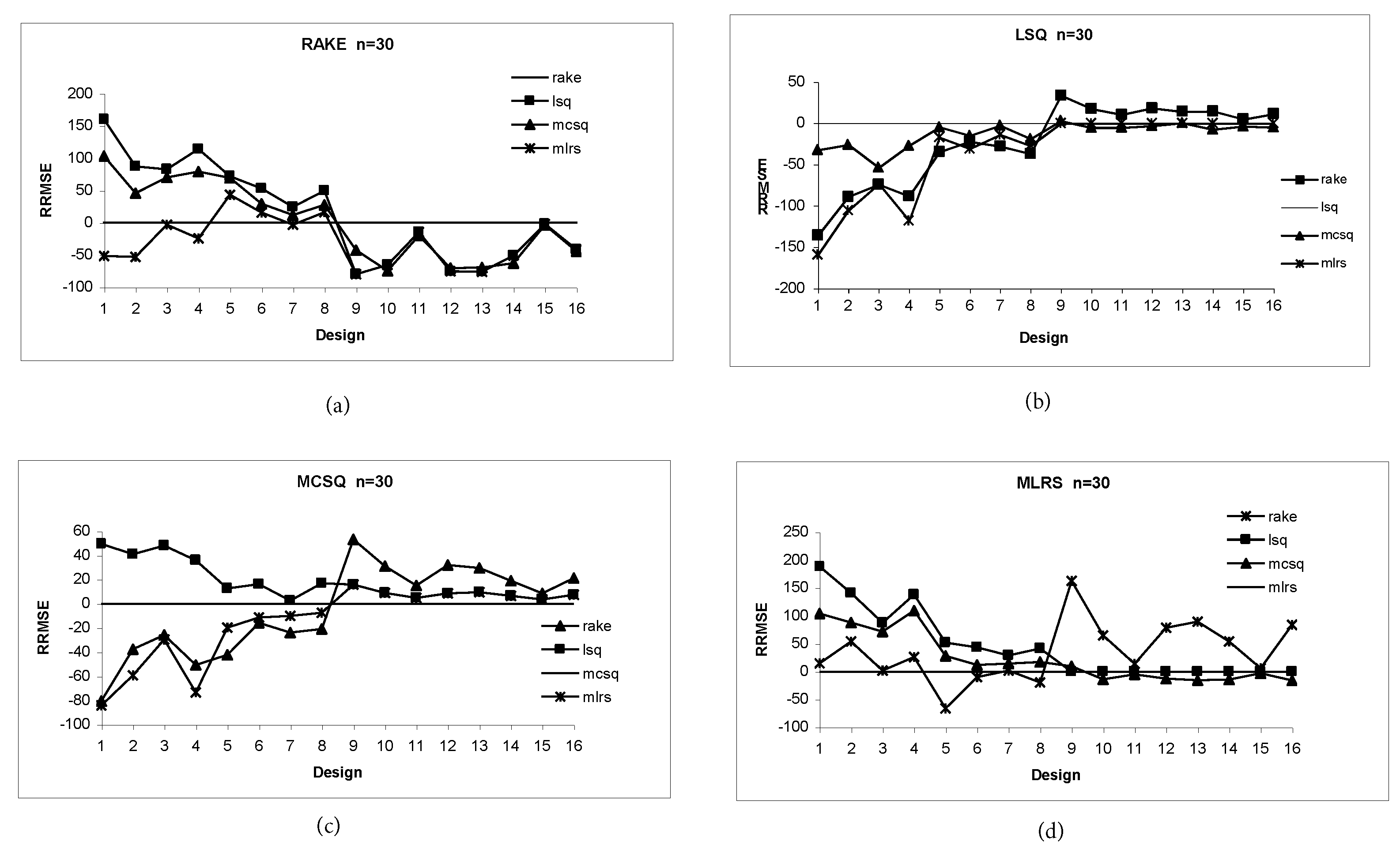
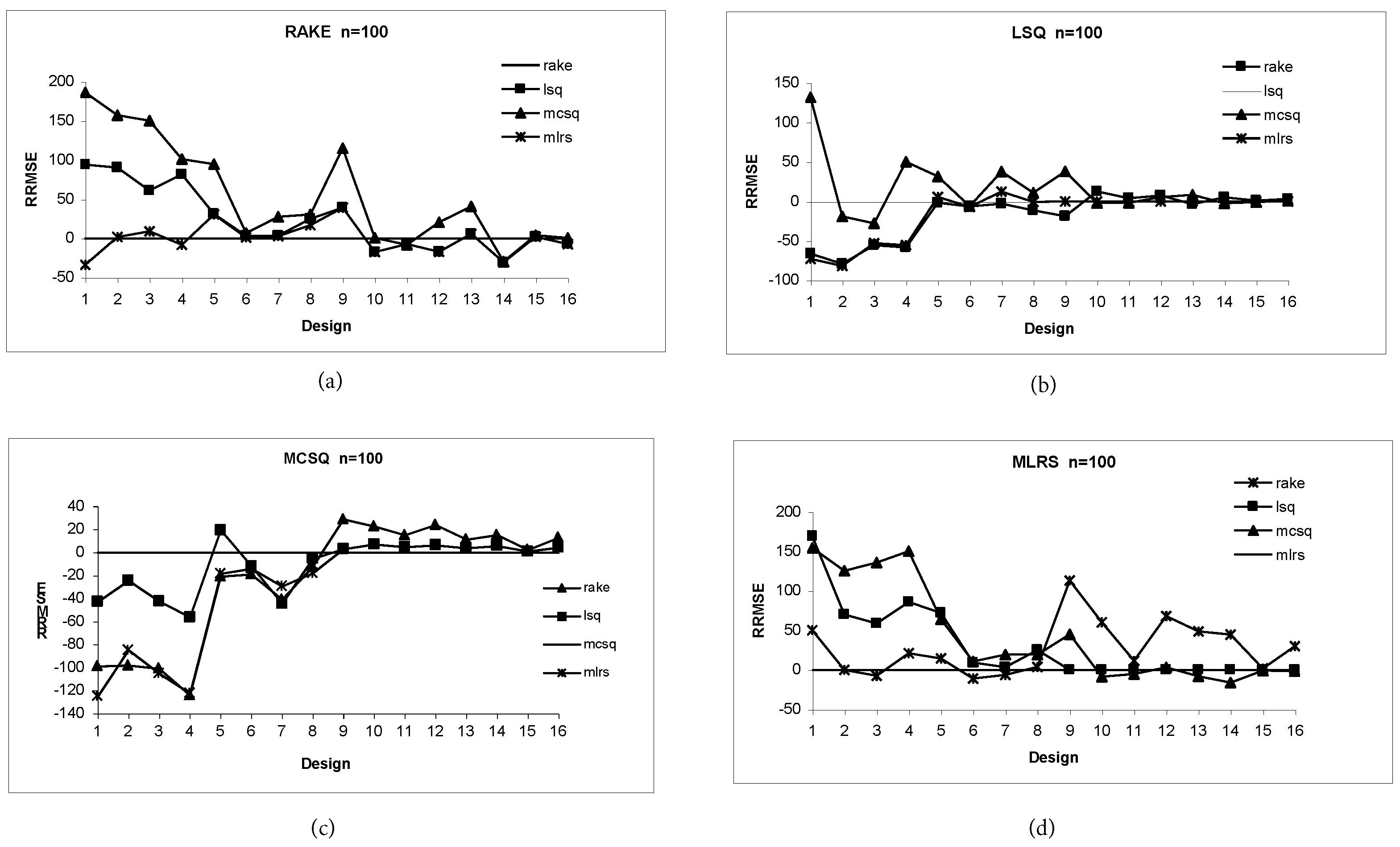
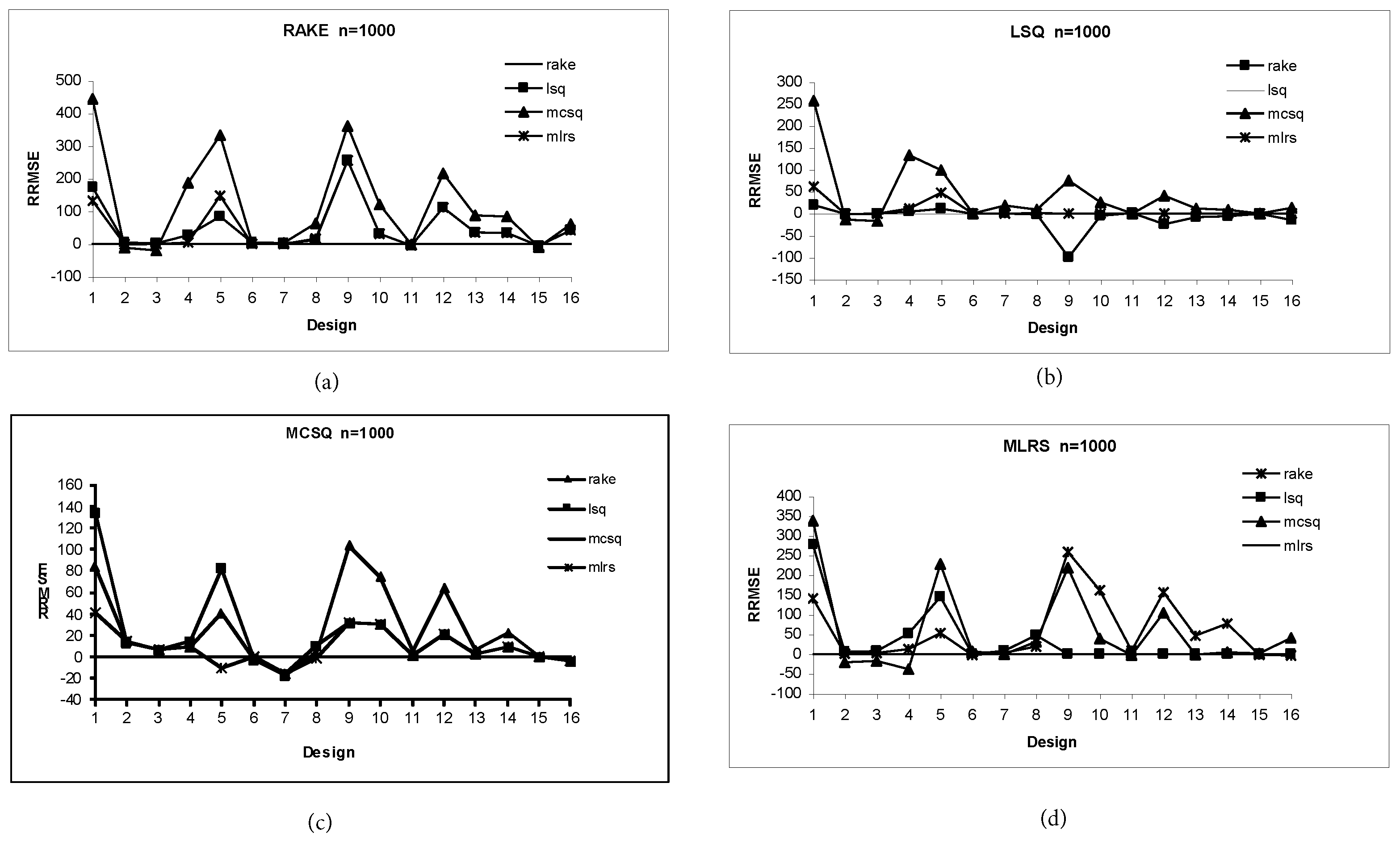
Figure 1, Figure 2 and Figure 3 give visual comparisons of the methods under each model, for sample sizes $n=30,100,1000$, respectively. For each figure the horizontal reference line with 0 RRMSE corresponds to the ML estimates under the model that was used to generate the data.

As mentoned earlier, for each sample size a total of 16 designs are considered, 1–8 are nonisotonic and 9–16 are isotonic; these are listed below. These designs are so numbered on the horizontal axis of each of the Figure 1, Figure 2 and Figure 3.

1. Nonisotonic; ${\pi }_{11}+{\pi }_{12}\le 0.4,{\pi }_{11}+{\pi }_{21}\le 0.4,\mathit{\pi }=(0.184,0.216,0.416,0.184)$ with $\mathit{\lambda }=(0.5,0.5)$; 2. ...$\mathit{\lambda }=(0,0.5)$; 3. ...$\mathit{\lambda }=(0.1,0.1)$; 4. ...$\mathit{\lambda }=(0.1,0.5)$; 5. Nonisotonic; ${\pi }_{11}+{\pi }_{12}\le 0.6,{\pi }_{11}+{\pi }_{21}\le 0.7,\mathit{\pi }=(0.387,0.213,0.313,0.087)$ with $\mathit{\lambda }=(0.5,0.5)$; 6. ...$\mathit{\lambda }=(0,0.5)$; 7. ...$\mathit{\lambda }=(0.1,0.1)$; 8. ...$\mathit{\lambda }=(0.1,0.5)$; 9. Isotonic; ${\pi }_{11}\le \{{\pi }_{12},{\pi }_{21}\},\mathit{\pi }=(0.232,0.232,0.232,0.304)$ with $\mathit{\lambda }=(0.5,0.5)$; 10. ...$\mathit{\lambda }=(0,0.5)$; 11. ...$\mathit{\lambda }=(0.1,0.1)$; 12. ...$\mathit{\lambda }=(0.1,0.5)$; 13. Isotonic; ${\pi }_{11}\le \{{\pi }_{12},{\pi }_{21}\},\mathit{\pi }=(0.231,0.303,0.264,0.202)$ with $\mathit{\lambda }=(0.5,0.5)$; 14. ...$\mathit{\lambda }=(0,0.5)$; 15. ...$\mathit{\lambda }=(0.1,0.1)$; 16. ...$\mathit{\lambda }=(0.1,0.5)$.

Overall RMSE of estimators. A crude comparison of the estimators is presented in

Table 2. Average root mean square error (RMSE) over all 16 designs by method and model that generated the data.

	Nonisotonic					Isotonic
	RAKE	LSQ	MCSQ	MLRS		RAKE	LSQ	MCSQ
Rake	0.0032	0.0061	0.0069	0.0034		0.0089	0.0063	0.0076
LSQ	0.0038	0.0060	0.0058	0.0038		0.0069	0.0062	0.0062
MCSQ	0.0037	0.0061	0.0054	0.0038		0.0077	0.0065	0.0061
MLRS	0.0033	0.0068	0.0061	0.0033		0.0109	0.0055	0.0054
RNDM	0.0039	0.0072	0.0069	0.0053		0.0084	0.0080	0.0078

, which gives the average RMSEs for each method over the 16 designs in each of isotonic and nonisotonic cases. Although the designs are different, this gives some illustration of the performance of the four methods. The RNDM values are obtained when the sample is taken directly from the target population. One would expect these values to be smaller than those that were generated from the sampled population, but we did not find that to be the case in our simulation study although they are pretty close.

When the target and sampled populations differ, one would expect that the method that is ML under the model that generated the data would have the lowest RMSE. For nonisotonic cases, RAKE satisfies this property; although MLRS does not satisfy this property, it follows RAKE closely. The RAKE estimates had the lowest RMSE under LSQ and MCSQ models as well. Thus, RAKE estimates seem to perform best, while MLRS follows RAKE very closely in each case. For the isotonic case, however, a different picture arises. Here, the LSQ estimates had the smallest RMSEs for the data generated under the RAKE model. Both LSQ and MCSQ estimates had the smallest RMSEs when the data were generated under the respective models. For MLRS, the MLRS estimates had slightly higher RMSEs than that of MCSQs.

Figure 1, Figure 2 and Figure 3 present RRMSEs for data generated under each of the four models for all 16 problems with n = 30, 100, 1000, respectively. To interpret them, first note that smaller values of $c_1,c_2$ mean stronger constraints. In addition, a negative value of RRMSE reflects that bias from model misspecification is represented by lower variance than the method that is ML for the model that generated the data.

Certain reasonable patterns emerge from these figures; estimates based on the correct model dominate other methods when the sample size is large, or when the constraints are isotonic; here, the bias from model misspecification dominates RMSE. Results from nonisotonic constraints are more homogeneous. For them, LSQ turned out to be generally larger than MLRS.

Panel a of the figures summarizes results for the data generated under the RAKE model. For nonisotonic constraints, RAKE and MLRS performed similarly. For n = 30, 100, LSQ is slightly inferior to the other methods for the nonisotonic constraints with $(c_1,c_2)=(0.4,0.6)$ but is competitive when $(c_1,c_2)=(0.6,0.7)$. RAKE seems to dominate (or close) and MCSQ performs worst (except when n = 30) of all nonisotonic constraints cases 1–8. RAKE performs slightly worse for isotonic constraints cases when n = 30, but is best again when n = 100, 1000.

Panel b of the figures summarizes results for data generated under the LSQ model. For all constraints with n 1000, LSQ and MLRS performed similarly. For n = 30, 100, LSQ is much inferior to MLRS for the nonisotonic constraints with $(c_1,c_2)=(0.4,0.6)$ but performs similarly when $(c_1,c_2)=(0.6,0.7)$. MCSQ performs worst throughout, except for isotonic constraints with n = 30, when all three methods did better than RAKE, but this turned around when n = 100, 1000.

Panel c of the figures summarizes results for the data generated under the MCSQ model. Although for isotonic constraints LSQ = MLRS, for nonisotonic constraints, LSQ performed much worse than MLRS. The MCSQ values were close to the LSQ values for all constraints, except for isotonic constraints designs 9, 12 with n = 1000 when MCSQ is way off. Rake performed competitively with MLRS for nonisotonic cases. However, for isotonic constraints, RAKE was outperformed by other three methods for all n.

Panel d of the figures summarizes results for data generated under the MLRS model. Although for isotonic constraints MCSQ performed best for all n, with nonisotonic constraints, MCSQ is beaten by all other methods for n = 100, and by RAKE and MLRS when n = 30. LSQ performed much worse than MLRS for all nonisotonic cases. MLRS performed best for nonisotonic constraints and was close to best (MCSQ) for isotonic constraints, for all n.

5. Applying Four Methods to Real World Data

In this section, we illustrate the four methods studied in this paper using the data from [3] on the second National Health and Nutrition Examination Survey (NHANES ⨿). The data are presented in Table 1.

It is not hard to observe that in Table 1a the sample cell and marginal proportions differ considerably from the census (see Section 1). From the census values for the income case from Table 1a, we see ${\pi }_{11}+{\pi }_{12}=0.3191$. Hence, it is reasonable to consider ${\pi }_{11}+{\pi }_{12}\le 0.32$; observing similar other discrepancies, we consider the following three inequality restrictions:

$$\left\{\begin{array}{c}{\pi }_{11}+{\pi }_{12}\le 0.32\\ {\pi }_{12}+{\pi }_{22}\le 0.30\\ {\pi }_{11}-2{\pi }_{12}\le 0\end{array},\right.$$

(10)

and for the education case, we consider

$$\left\{\begin{array}{c}{\pi }_{11}+{\pi }_{12}\le .67\\ {\pi }_{11}+{\pi }_{21}\ge .72\end{array}.\right.$$

(11)

For each problem, the estimates and RMSEs are computed and the results are displayed in

Table 3. Proportional unexplained root mean square error (PURMSE) values for different methods under inequality restrictions for Income and education.

Variable	RAKE	LSQ	MCSQ	MLRS
Income	92.88	92.88	98.50	96.84
Education	94.58	88.36	93.96	94.24

. We consider the census proportions as the target probabilities $\left\{{\pi }_{ij}\right\}$.

Let NHANES ⨿ data be our sample proportions $\left\{p_{ij}\right\}$. Let $\left\{{\widehat{\pi }}_{ij}\right\}$ be the estimates under the constraints in (10), also under (11) (considered separately). Below, we define the adjusted RMSE, the unadjusted RMSE, and the proportional unexplained root mean square error (PURMSE), where “adjusted” means estimates under constraints, and “unadjusted” means unrestricted sample proportions.

$$adjustedRMSE=\sqrt{\sum _i\sum _j{({\widehat{\pi }}_{ij}-{\pi }_{ij})}^2},$$

(12)

$$unadjustedRMSE=\sqrt{\sum _i\sum _j{(p_{ij}-{\pi }_{ij})}^2},$$

(13)

$$PURMSE=100*\frac{unadjustedRMSE-adjustedRMSE}{unadjustedRMSE}.$$

(14)

The larger value of PURMSE means that the adjusted MSEs are smaller than the unadjusted, which subsequently means that the used constraints give estimates that are quite close to the target values. Table 3 shows that all four methods perform well. Among all methods, LSQ performs comparatively the worst.

6. Conclusions

The paper [3] compared four margin-adjusting methods using equality constraints of known marginal totals for $(I\times J)$ contingency tables. Here, under general linear inequality constraints, theoretical models are proposed for the differences between the sampled and target populations. To compare the performance of these four methods, a simulation is performed for the case of $I=J=2$. Based on this simulation, we find that the performance of the methods depends on the specific type of constraints. For nonisotonic constraints, we find RAKE to perform the best, with MLRS being a close second. The MCSQ and LSQ perform worse, of which MCSQ is slightly better than LSQ. These findings are parallel to those of [3].

However, we also find that the performance ranking of the methods changes for isotonic constraints (tree order). Here, MCSQ and LSQ (= MLRS) perform better than RAKE. In addition, MCSQ is slightly better than LSQ (= MLRS). These results are very different from those of [3].

The theoretical models for the differences between the sampled and target populations, and the corresponding methods and techniques described can be extended to higher dimensions in a similar manner as in Theorem 1.

As opposed to the case under equality restrictions, the distribution of estimators under inequality constraints is not known; hence, their mean and standard errors are also not tractable. It is difficult to explain the different behavior of the estimators under isotonic and non-isotonic constraints as seen in simulation. It is well-known that estimators under isotonic constraints have special properties of partial order relations.

We have fixed the values of $c_1,c_2$ earlier in the simulation keeping in par with applications. This makes the choices of ${\pi }_{ij}$ restricted under inequality constraints. Note that with equality constraints, once we fix ${\pi }_{11}$, all values of ${\pi }_{ij}$ are fixed. This is not the case under inequality constraints. The choices of ${\pi }_{ij},{\lambda }_i$ have to be such that the optimization problem has a solution.

References

1. Causey, B.D. Estimation under generalized sampling of cell proportions for contingency tables subject to marginal constraints. Commun. Stat. Theory Meth. 1984, 13, 2487–2494. [Google Scholar] [CrossRef]
2. Read, T.R.C.; Cressie, N. Goodness-of-fit Statistics for Discrete Multivariate Data; Springer: New York, NY, USA, 1988. [Google Scholar]
3. Little, R.J.A.; Wu, M.-M. Models for contingency tables with known margins when target and sampled populations differ. J. Am. Stat. Assoc. 1991, 86, 87–95. [Google Scholar] [CrossRef]
4. Hellerstein, J.K.; Imbens, G.W. Imposing moment restrictions from auxiliary data by weighting. Rev. Econ. Stat. 1996, 81, 1–14. [Google Scholar] [CrossRef]
5. Causey, B.D. Estimation of proportions for multinomial contingency tables subject to known marginal constraints. Commun. Stat. Theory Meth. 1983, 12, 2581–2587. [Google Scholar] [CrossRef]
6. Rockafellar, R.T. Convex Analysis; John Wiley & Sons, Inc.: New York, NY, USA, 1970. [Google Scholar]
7. Robertson, T.; Wright, F.T.; Dykstra, R.L. Order Restricted Statistical Inference; John Wiley & Sons, Inc.: New York, NY, USA, 1988. [Google Scholar]
Figure 1. RRMSEs for data generated under four models (a) RAKE, (b) LSQ, (c) MCSQ, (d) MLRS, when n = 30 . The horizontal reference line at 0 RRMSE corresponds to ML estimates under the model.
Entropy 18 00097 g001
Figure 2. RRMSEs for data generated under four models (a) RAKE, (b) LSQ, (c) MCSQ, (d) MLRS, when n = 100 . The horizontal reference line at 0 RRMSE corresponds to ML estimates under the model.
Entropy 18 00097 g002
Figure 3. RRMSEs for data generated under four models (a) RAKE, (b) LSQ, (c) MCSQ, (d) MLRS, when n = 1000 . The horizontal reference line at 0 RRMSE corresponds to ML estimates under the model.
Entropy 18 00097 g003