
Riemannian Laplace Distribution on the Space of Symmetric Positive Definite Matrices


 and
and 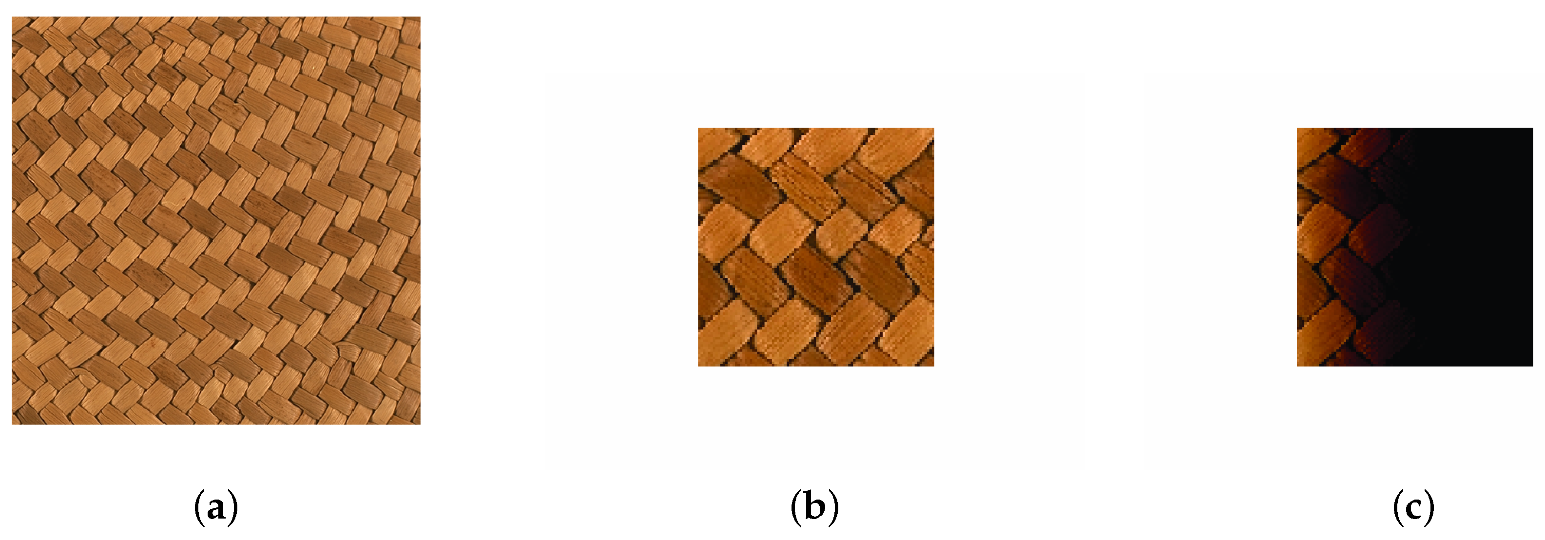
Abstract
:1. Introduction
2. Riemannian Geometry of
3. Riemannian Laplace Distribution on
3.1. Definition of
3.2. Sampling from
| Algorithm 1 Sampling from . |
|
3.3. Estimation of and σ
- (i)
- is given by:That is, is the Riemannian median of .
- (ii)
- σ is given by:where the function Φ is the inverse function of .
4. Mixtures of Laplace Distributions
4.1. Estimation of the Mixture Parameters
- Update for : Based on the current value of , assign to the new value
- Update for : Based on the current value of , assign to the value:
- Update for : Based on the current value of , assign to the new value:
4.2. The Bayesian Information Criterion
5. Application to Classification of Data on
5.1. Classification Using Mixtures of Laplace Distributions
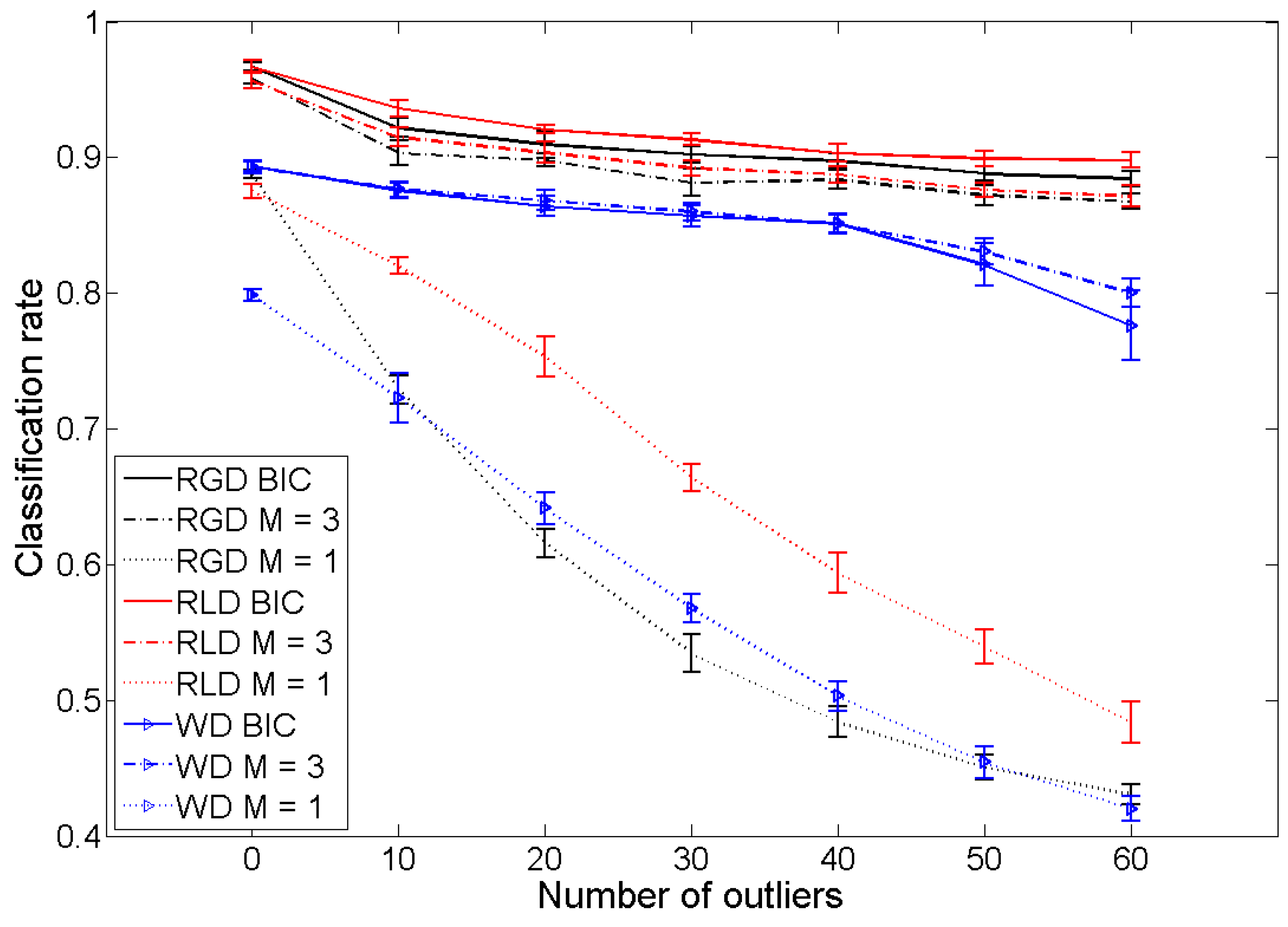
5.2. Application to Texture Classification
6. Conclusions
Acknowledgments
Author Contributions
Conflicts of Interest
Appendix: Proofs of Some Technical Points
A. Derivation of Equation (16) from Equation (14)
B. Derivation of Equation (19)
C. The Normalizing Factor
- (i)
- for all ;
- (ii)
- .
D. The Law of X in Algorithm 1
References
- Pennec, X.; Fillard, P.; Ayache, N. A Riemannian framework for tensor computing. Int. J. Comput. Vis. 2006, 66, 41–66. [Google Scholar] [CrossRef] [Green Version]
- Barachant, A.; Bonnet, S.; Congedo, M.; Jutten, C. Multiclass Brain–Computer Interface Classification by Riemannian Geometry. IEEE Trans. Biomed. Eng. 2012, 59, 920–928. [Google Scholar] [CrossRef] [PubMed] [Green Version]
- Jayasumana, S.; Hartley, R.; Salzmann, M.; Li, H.; Harandi, M. Kernel Methods on the Riemannian Manifold of Symmetric Positive Definite Matrices. In Proceedings of the IEEE Conference on Computer Vision and Pattern Recognition (CVPR), Portland, OR, USA, 23–28 June 2013; pp. 73–80.
- Zheng, L.; Qiu, G.; Huang, J.; Duan, J. Fast and accurate Nearest Neighbor search in the manifolds of symmetric positive definite matrices. In Proceedings of the IEEE International Conference on Acoustics, Speech and Signal Processing (ICASSP), Florence, Italy, 4–9 May 2014; pp. 3804–3808.
- Dong, G.; Kuang, G. Target recognition in SAR images via classification on Riemannian manifolds. IEEE Geosci. Remote Sens. Lett. 2015, 21, 199–203. [Google Scholar] [CrossRef]
- Tuzel, O.; Porikli, F.; Meer, P. Pedestrian detection via classification on Riemannian manifolds. IEEE Trans. Pattern Anal. Mach. Intell. 2008, 30, 1713–1727. [Google Scholar] [CrossRef] [PubMed]
- Caseiro, R.; Henriques, J.F.; Martins, P.; Batista, J. A nonparametric Riemannian framework on tensor field with application to foreground segmentation. Pattern Recognit. 2012, 45, 3997–4017. [Google Scholar] [CrossRef]
- Arnaudon, M.; Barbaresco, F.; Yang, L. Riemannian Medians and Means With Applications to Radar Signal Processing. IEEE J. Sel. Top. Signal Process. 2013, 7, 595–604. [Google Scholar] [CrossRef]
- Arnaudon, M.; Yang, L.; Barbaresco, F. Stochastic algorithms for computing p-means of probability measures, Geometry of Radar Toeplitz covariance matrices and applications to HR Doppler processing. In Proceedings of International International Radar Symposium (IRS), Leipzig, Germany, 7–9 September 2011; pp. 651–656.
- Terras, A. Harmonic Analysis on Symmetric Spaces and Applications; Springer-Verlag: New York, NY, USA, 1988; Volume II. [Google Scholar]
- Atkinson, C.; Mitchell, A. Rao’s distance measure. Sankhya Ser. A 1981, 43, 345–365. [Google Scholar]
- Pennec, X. Probabilities and statistics on Riemannian manifolds: Basic tools for geometric measurements. In Procedings of the IEEE Workshop on Nonlinear Signal and Image Processing, Antalya, Turkey, 20–23 June 1999; pp. 194–198.
- Pennec, X. Intrinsic statistics on Riemannian manifolds: Basic tools for geometric measurements. J. Math. Imaging Vis. 2006, 25, 127–154. [Google Scholar] [CrossRef]
- Guang, C.; Baba, C.V. A Novel Dynamic System in the Space of SPD Matrices with Applications to Appearance Tracking. SIAM J. Imaging Sci. 2013, 6, 592–615. [Google Scholar]
- Said, S.; Bombrun, L.; Berthoumieu, Y.; Manton, J. Riemannian Gaussian distributions on the space of symmetric positive definite matrices. 2015; arXiv:1507.01760. [Google Scholar]
- Schwarz, G. Estimating the Dimension of a Model. Ann. Stat. 1978, 6, 461–464. [Google Scholar] [CrossRef]
- Lee, J.S.; Grunes, M.R.; Ainsworth, T.L.; Du, L.J.; Schuler, D.L.; Cloude, S.R. Unsupervised classification using polarimetric decomposition and the complex Wishart classifier. IEEE Trans. Geosci. Remote Sens. 1999, 37, 2249–2258. [Google Scholar]
- Berezin, F.A. Quantization in complex symmetric spaces. Izv. Akad. Nauk SSSR Ser. Mat. 1975, 39, 363–402. [Google Scholar] [CrossRef]
- Malliavin, P. Invariant or quasi-invariant probability measures for infinite dimensional groups, Part II: Unitarizing measures or Berezinian measures. Jpn. J. Math. 2008, 3, 19–47. [Google Scholar] [CrossRef]
- Barbaresco, F. Information Geometry of Covariance Matrix: Cartan-Siegel Homogeneous Bounded Domains, Mostow/Berger Fibration and Fréchet Median, Matrix Information Geometry; Bhatia, R., Nielsen, F., Eds.; Springer: New York, NY, USA, 2012; pp. 199–256. [Google Scholar]
- Barbaresco, F. Information geometry manifold of Toeplitz Hermitian positive definite covariance matrices: Mostow/Berger fibration and Berezin quantization of Cartan-Siegel domains. Int. J. Emerg. Trends Signal Process. 2013, 1, 1–11. [Google Scholar]
- Jeuris, B.; Vandebril, R. Averaging block-Toeplitz matrices with preservation of Toeplitz block structure. In Proceedings of the SIAM Conference on Applied Linear Algebra (ALA), Atlanta, GA, USA, 20–26 October 2015.
- Jeuris, B.; Vandebril, R. The Kähler Mean of Block-Toeplitz Matrices with Toeplitz Structured Block. Available online: http://www.cs.kuleuven.be/publicaties/rapporten/tw/TW660.pdf (accessed on 10 March 2016).
- Jeuris, B. Riemannian Optimization for Averaging Positive Definite Matrices. Ph.D. Thesis, University of Leuven, Leuven, Belgium, 2015. [Google Scholar]
- Maass, H. Siegel’s modular forms and Dirichlet series. In Lecture Notes in Mathematics; Springer-Verlag: New York, NY, USA, 1971; Volume 216. [Google Scholar]
- Higham, N.J. Functions of Matrices, Theory and Computation; Society for Industrial and Applied Mathematics: Philadelphia, PA, USA, 2008. [Google Scholar]
- Helgason, S. Differential Geometry, Lie Groups, and Symmetric Spaces; American Mathematical Society: Providence, RI, USA, 2001. [Google Scholar]
- Afsari, B. Riemannian Lp center of mass: Existence, uniqueness and convexity. Proc. Am. Math. Soc. 2011, 139, 655–673. [Google Scholar] [CrossRef]
- Muirhead, R.J. Aspects of Multivariate Statistical Theory; John Wiley & Sons: New York, NY, USA, 1982. [Google Scholar]
- Robert, C.P.; Casella, G. Monte Carlo Statistical Methods; Springer-Verlag: Berlin, Germany, 2004. [Google Scholar]
- Udriste, C. Convex Functions and Optimization Methods on Riemannian Manifolds; Mathematics and Its Applications; Kluwer Academic Publishers: Dordrecht, The Netherlands, 1994. [Google Scholar]
- Chavel, I. Riemannian Geometry, a Modern Introduction; Cambridge University Press: Cambridge, UK, 2006. [Google Scholar]
- Yang, L. Médianes de Mesures de Probabilité dans les Variétés Riemanniennes et Applications à la Détection de Cibles Radar. Ph.D. Thesis, L’université de Poitiers, Poitiers, France, 2011. [Google Scholar]
- Li, Y.; Wong, K.M. Riemannian distances for signal classification by power spectral density. IEEE J. Sel. Top. Sig. Process. 2013, 7, 655–669. [Google Scholar] [CrossRef]
- Hastie, T.; Tibshirani, R.; Friedman, J. The Elements of Statistical Learning: Data Mining, Inference, and Prediction; Springer: Berlin, Germany, 2009. [Google Scholar]
- Saint-Jean, C.; Nielsen, F. A new implementation of k-MLE for mixture modeling of Wishart distributions. In Geometric Science of Information (GSI); Springer-Verlag: Berlin/Heidelberg, Germany, 2013; pp. 249–256. [Google Scholar]
- Hidot, S.; Saint-Jean, C. An expectation-maximization algorithm for the Wishart mixture model: Application to movement clustering. Pattern Recognit. Lett. 2010, 31, 2318–2324. [Google Scholar] [CrossRef]
- VisTex: Vision Texture Database. MIT Media Lab Vision and Modeling Group. Available online: http://vismod.media.mit.edu/pub/ (accessed on 9 March 2016).
- Daubechies, I. Ten Lectures on Wavelets; Society for Industrial and Applied Mathematics: Philadelphia, PA, USA, 1992. [Google Scholar]
- Do, M.N.; Vetterli, M. Wavelet-Based Texture Retrieval Using Generalized Gaussian Density and Kullback-Leibler Distance. IEEE Trans. Image Process. 2002, 11, 146–158. [Google Scholar] [CrossRef] [PubMed]
- Bombrun, L.; Berthoumieu, Y.; Lasmar, N.-E.; Verdoolaege, G. Mutlivariate Texture Retrieval Using the Geodesic Distance between Elliptically Distributed Random Variables. In Proceedings of 2011 18th IEEE International Conference on Image Processing (ICIP), Brussels, Belgium, 11–14 September 2011.
- Verdoolaege, G.; Scheunders, P. On the Geometry of Multivariate Generalized Gaussian Models. J. Math. Imaging Vis. 2012, 43, 180–193. [Google Scholar] [CrossRef]
- Stitou, Y.; Lasmar, N.-E.; Berthoumieu, Y. Copulas based Multivariate Gamma Modeling for Texture Classification. In Proceedings of the IEEE International Conference on Acoustic Speech and Signal Processing, Taipei, Taiwan, 19–24 April 2009; pp. 1045–1048.
- Kwitt, R.; Uhl, A. Lightweight Probabilistic Texture Retrieval. IEEE Trans. Image Process. 2010, 19, 241–253. [Google Scholar] [CrossRef] [PubMed]


© 2016 by the authors; licensee MDPI, Basel, Switzerland. This article is an open access article distributed under the terms and conditions of the Creative Commons by Attribution (CC-BY) license (http://creativecommons.org/licenses/by/4.0/).
Share and Cite
Hajri, H.; Ilea, I.; Said, S.; Bombrun, L.; Berthoumieu, Y. Riemannian Laplace Distribution on the Space of Symmetric Positive Definite Matrices. Entropy 2016, 18, 98. https://0-doi-org.brum.beds.ac.uk/10.3390/e18030098
Hajri H, Ilea I, Said S, Bombrun L, Berthoumieu Y. Riemannian Laplace Distribution on the Space of Symmetric Positive Definite Matrices. Entropy. 2016; 18(3):98. https://0-doi-org.brum.beds.ac.uk/10.3390/e18030098
Chicago/Turabian StyleHajri, Hatem, Ioana Ilea, Salem Said, Lionel Bombrun, and Yannick Berthoumieu. 2016. "Riemannian Laplace Distribution on the Space of Symmetric Positive Definite Matrices" Entropy 18, no. 3: 98. https://0-doi-org.brum.beds.ac.uk/10.3390/e18030098