Mixed Diffusive-Convective Relaxation of a Warm Beam of Energetic Particles in Cold Plasma

Abstract

This work addresses the features of fast particle transport in the bump-on-tail problem for varying the width of the fluctuation spectrum, in the view of possible applications to studies of energetic particle transport in fusion plasmas. Our analysis is built around the idea that strongly-shaped beams do not relax through diffusion only and that there exists an intermediate time scale where the relaxations are convective (ballistic-like). We cast this idea in the form of a self-consistent nonlinear dynamical model, which extends the classic equations of the quasi-linear theory to “broad” beams with internal structure. We also present numerical simulation results of the relaxation of a broad beam of energetic particles in cold plasma. These generally demonstrate the mixed diffusive-convective features of supra-thermal particle transport essentially depending on nonlinear wave-particle interactions and phase-space structures. Taking into account the modes of the stable linear spectrum is crucial for the self-consistent evolution of the distribution function and the fluctuation intensity spectrum.

1. Introduction

The relaxation of supra-thermal particle beams in plasmas is a problem of fundamental significance. Dating back to the 1960s, it provides a paradigm for the quasi-linear theory of weak plasma turbulence [1,2], which finds applications in a wide field ranging from astrophysics and cosmical geo-physics [3,4] to fusion plasma [4,5]. Its original important promotion is due to Bernstein, Greene and Kruskal (BGK), whose seminal work in [6] has come to be known as the classic “bump-on-tail” (BoT) problem. Specific implications concern Landau damping [7,8] and nonlinear behavior of the beam-plasma instability driven by wave-particle interactions [5,9,10] (see also [11,12,13,14,15,16]). The “perturbation theory of strong plasma turbulence”, originally proposed by Dupree [17] and illuminating resonance broadening by fluctuation-induced stochastic particle motion, also ought to be mentioned for its importance and crucial implications in plasma research.

The relevance of the BoT problem for fusion plasma research was revived in the 1990s by Berk and Breizman [18,19,20], who proposed it as a paradigmatic model to investigate and understand the nonlinear interaction of supra-thermal particles with Alfvén fluctuations [20,21,22,23]. In fact, the nonlinear interplay of energetic particles (EPs) with Alfvénic fluctuations (such as Alfvén eigenmodes (AEs), EP modes and drift Alfvén waves [21,22,24,25]) and their consequences for fluctuation-induced cross-field transport constitute basic phenomena for thermonuclear plasmas [23,25,26,27,28,29,30,31,32,33,34,35].

The fluctuation spectrum of AEs, EP-driven modes and drift Alfvén waves in fusion plasmas covers disparate spatiotemporal scales and can have both “broad” features, such as those of typical plasma turbulence, as well as an almost “coherent” (“narrow”), nearly periodic component [24,33]. A line-broadened quasi-linear approach has been proposed in [36,37] for computing EP transport by means of a diffusion equation, which could address not only overlapping resonant Alfvénic fluctuations, but also the broadening of the resonant spectrum for isolated instabilities in the case of multiple AEs. This model has been extended and compared to experimental observations [38] and to numerical solutions of the BoT paradigm [39]. In general, however, understanding the complex features of EP transport in fusion plasmas requires going beyond the local description of fluctuation-induced fluxes and extending the diffusive transport paradigm [24,33]. Accounting for modes of the linear stable spectrum is also crucial [40,41]. Thus, posing these issues for the BoT problem becomes an interesting and relevant research topic, in light of its possible implications as a paradigm for Alfvénic fluctuation-induced supra-thermal particle transport in fusion plasmas near marginal stability. In particular, a relevant question to pose is assessing the changing behavior of EP transport when properties of the fluctuation spectrum are modified from “narrow” (nearly periodic or coherent) to “broad” (turbulent). This is the main focus of the present work. Non-diffusive processes could also be of interest in various other areas of research. For example in the energy extraction from plasmas (see, e.g., [42,43] and the references therein for a recent discussion of the energy extraction problem); and in the light power absorption by plasmas [44,45], where meso-scale convective (coherent) phenomena may generate relevant effects.

The issues addressed in the present work clearly have common aspects with important and well-known results of the vast BoT literature. More precisely, we deal with resonant wave-coupling mediated by resonant particles, which is summarized and explained in the review work by Laval and Pesme [46]. For sufficiently strong nonlinearity, such that resonance broadening dominates over the linear growth rate, renormalization of the propagator yields to wave-coupling terms that are of the same order of quasi-linear diffusion and must be taken into account, as explained by the turbulent trapping model (TTM) [47]. In general, phase-space structures and, thereby, nonlinear wave-particle interactions are known to be important, e.g., in enhancing velocity space diffusion due to longitudinal plasma turbulence [48,49,50]. Most of the existing literature deals with “broad” turbulent fluctuation spectra. In this work, meanwhile, we address the role of nonlinearity in supra-thermal particle transport by a fluctuation spectrum that is not necessarily “broad”. We revisit the implications of the classic BoT problem and demonstrate the occurrence of the relaxation dynamics of the convective type on intermediate (meso-) time scales (other than the familiar asymptotic velocity-space diffusion and the formation of the plateau [1,2,5]). Our results elucidate the crucial role played by the wave-particle nonlinear interaction in determining transport in phase space both on meso- and asymptotic time scales.

The paper is organized as follows. First, we touch on the classic BoT problem in brief (Section 2), with particular attention to the causes and origins of the stochastic behavior of the resonant particles. In Section 3, we formulate a mixed convection-diffusion model of velocity space transport, which extends the familiar quasi-linear diffusion to relaxation processes in the presence of many overlapping resonances. We discuss the similarities and differences of our approach with the well-established theoretical framework of the classic BoT problem, including its aforementioned subtleties connected with a sufficiently strong nonlinearity. Mathematically, the model in Section 3 relies on the formalism of the Klein–Kramers equation with a force-field (if external or effectively self-organized) and incorporates the various exclusions from pure diffusive style models. Numerical simulation results are collected in Section 4, where one also finds a Hamiltonian formulation of the BoT problem based on [51]. There, four different cases are presented and discussed, changing the strength of the nonlinearity parameter and the width of the fluctuation spectrum. It is shown numerically that convective relaxation takes place on meso-scales for strong nonlinearity and a sufficiently broad spectrum, in contrast to the narrow spectrum case, dominated by coherent structures. Convective relaxation is also found to occur for small nonlinearity parameter as a result of a self-consistent evolution of the fluctuation spectrum on the same time scales of particle transport. We support these findings with a simplified theory model. Finally, Section 5 is devoted to the summary and conclusions.

2. The Classic “Bump-On-Tail” Problem and the Brownian Random-Walk Paradigm

We will assume that the reader is familiar with the classic BoT problem [6] of a distribution function that excites electrostatic waves. The basic insight is that the velocity space gradient drives (damps) the instabilities via the Cherenkov resonance $v=v_{res}={\omega }_{k_j}/k_j$ with the plasma species (customarily associated with the energetic electrons). Here, v is the particle velocity, and ${\omega }_{k_j}$ and $k_j$ are, respectively, the frequency and the wave-vector of the resonant mode. Instability occurs when the gradient is positive ($\partial f/\partial v>0$) and is damped when it is negative ($\partial f/\partial v<0$). The latter phenomenon is known as the Landau damping and in many ways is the inversion of the BoT problem (by “velocity distribution” we mean the probability density, $f=f(v,t)$, of finding a particle at time t with a velocity value between v and $v+dv$ regardless of its position in real space).

In the quasi-linear theory [1,2,5] of weak plasma turbulence, one assumes that the electron distribution function contains a small “bump” in the parameter range of large energies (much larger than the characteristic thermal energy) and that the dispersion of the electron velocities is also large compared to the thermal velocity. The bump being small implies that the level of the excited electrostatic noises is so low that the different unstable modes do not interact; hence, one neglects any nonlinearities in the wave-field. Then, the only nonlinearity one indeed takes into account is the feedback effect of the waves onto the averaged velocity distribution function (hence, the name of this theory: quasi-linear). The linear instability growth rate, which is frequency and wave-vector dependent, is given by:

$${\gamma }_{k_j}=\frac{\pi {\omega }_p^3}{2k_j^2{n}_p}\frac{\partial f}{\partial v}{|}_{v_{res}},$$

(1)

where ${\omega }_p$ is the unperturbed Langmuir frequency (i.e., ${\omega }_p\equiv \sqrt{4\pi n_p{e}^2/m_e}$, with $n_p$ the thermal plasma density; and $m_e$ and e denoting the mass and charge of electrons, respectively) and the gradient in the velocity space is taken at the Cherenkov resonance exactly. The large velocity dispersion within the bump is at the basis of another important assumption of the quasi-linear theory, namely that the number of the excited modes is so large that their phases are represented by the random functions. Then, the kicks received by the plasma particles via the resonant interactions with the waves will be also random in the limit $t\to \infty$ (here, t is the time). It is generally believed that this quasi-linear effect of the many excited waves onto the plasma is contained in a Brownian random walk of the energetic particles toward the thermal core and the formation of a characteristic “plateau” ($\partial f/\partial v=0$) in the equilibrium velocity distribution function [1,2].

The conclusion that the transport in the velocity space is diffusive or Brownian random walk-like is however not at all trivial and should be addressed. It occurs as a consequence of the idea that the resonant particles are not caught by one single resonance on time scales longer than a certain characteristic time (thought of as the typical bouncing time in the potential well of the wave). Instead, these particles will hop in a random fashion between the many overlapping resonances; hence, their motion is statistical, rather than deterministic. This statistical approach to the particle random motion in the velocity space is well documented in books and reviews (e.g., [3,4,52,53] due to the Novosibirsk school of nonlinear science).

Consider the exact equations of motion of a charged particle in the potential electric field of a wave packet:

$$\ddot{x}=\frac{e}{m_e}E(x,t)=\frac{e}{m_e}\sum _j\left[E_{k_j}{e}^{i(k_{j}x-{\omega }_{k_j}t)}+c.c.\right],$$

(2)

where $\dot{x}=v$ is the particle velocity and $E_{k_j}$ is the Fourier amplitude of a mode with wave-vector $k_j$. The electric field is assumed to be “small” in the sense of quasi-linear theory; and here, it is represented as the sum of a large number of Fourier harmonics with frequencies ${\omega }_{k_j}$ and wave-vectors $k_j$. Hence, it is shown, following Zaslavsky [3], that barely trapped particles, those staying close to separatrices in phase space $(x,\dot{x})$, may occasionally become detrapped by jumping onto an open trajectory. These phenomena of occasional trapping-detrapping occur because the integrals of the motion are essentially destroyed by the perturbation $E(x,t)$ within a small layer surrounding the separatrix (known as the ergodic layer) [3,4]. For not too small perturbations, the width of the ergodic layer with respect to frequency is of the order of:

$$\Delta {\omega }_{k_j}=\sqrt{\frac{ek|E_{k_j}|}{m_e}}.$$

(3)

The diffusion behavior occurs when the width $\Delta {\omega }_{k_j}$ exceeds by a large margin the distance between the resonances $\delta {\omega }_{k_j}$ (for a statistically-significant number of k’s), implying that the resonances strongly overlap within a certain interval of wave-vectors $k_j$. This is usually quantified by saying that the Chirikov parameter is large [54], i.e.,

$$\mathcal{S}=\Delta {\omega }_{k_j}/\delta {\omega }_{k_j}\gg 1.$$

(4)

One sees that the Chirikov parameter $\mathcal{S}\propto \sqrt{|E_{k_j}|}$ being much larger than one implies that the level of the excited electrostatic waves in turn cannot be as small as one likes. It might not be taken for granted that this level just lies within the assumptions of the quasi-linear theory discussed above, even though we know by experience that the conflict does not normally occur in the classic BoT setting.

3. Revising the Classic “Bump-On-Tail” Problem: Diffusion-Convection Model

We are now in a position to revisit the implication of velocity space diffusion as a paradigmatic model of the beam relaxation in cold plasma. The main idea here is that large-amplitude or strongly-shaped beams do not relax through diffusion only and that there exists an intermediate time scale where the relaxations are “convective” (ballistic-like). We cast this idea in the form of a self-consistent nonlinear dynamical model, i.e., mixed diffusion-convection model, which aims at generalizing the classic equations of the quasi-linear theory to “broad” (warm) beams with internal structure.

We shall assume for simplicity, without loss of generality, that the density of the beam particles is small compared to the density of the background plasma, and we neglect, accordingly, the possible perturbations to quasi-neutrality (and the associated ambipolar electric field) due to the beam injection.

Next, we consider a “broad” beam as composed of a large number of overlapping single cold beams, each having a characteristic nonlinear width $\Delta v^{NL}$ and the spacing between the beams represented by $\Delta v^{SEP}$. The value of $\Delta v^{NL}$ is determined by the kinematics of nonlinear resonance broadening in the coupled system of electrostatic waves and beam-plasma particles (e.g., [4,55]). The behavior crucially depends on the value of the nonlinearity parameter:

$$K=\Delta v^{NL}/\Delta v^{SEP}.$$

(5)

Here, $\Delta v^{NL}$ can be estimated as $\Delta v^{NL}\sim (\Delta {\omega }_k^2/k){\tau }_s$, with ${\tau }_s=1/(k\Delta v)$ the “autocorrelation time”, that is the time for particles to be scattered by randomization with respect to wave phases. Note that the nonlinearity parameters in Equation (4) and Equation (5) are connected as $K\simeq \mathcal{S}/Q\equiv {\mathcal{S}}^2/\Delta \ell$, with $\Delta \ell =(L/2\pi )\Delta k$ being a measure of the fluctuation spectrum width ($\Delta k$), L the macroscopic system size and:

$$\begin{array}{c}\hfill Q={({\tau }_s\Delta {\omega }_k)}^{-1}=\Delta \ell /\mathcal{S}.\end{array}$$

(6)

We also note that another nonlinearity parameter $R={({\gamma }_k{\tau }_{nl})}^{-3}$ (with ${\tau }_{nl}={(k^2{D}_{QL})}^{-1/3}$ [17,54] and $D_{QL}$ denoting the quasi-linear diffusion coefficient) can be introduced for measuring the strength of wave-coupling effects [46,47] and could also be expressed, here, as $R\sim 2\pi \mathcal{S}{(\Delta {\omega }_k/{\gamma }_k)}^3$ (cf. also Section 4.2). For large R (and $\mathcal{S}$), Laval and Pesme derived the TTM for a “broad” turbulent spectrum ($\Delta \ell \gg 1$) [47] and demonstrated that the growth rate and diffusion coefficient are expected to be increased with respect to the quasi-linear estimate. These results are typically meant to describe the condition $K\ll 1$, where the propagator renormalization yields the corresponding correction to $D_{QL}$ [46].

The behavior changes if $K\gtrsim 1$. In this parameter range, the beams strongly overlap as a consequence of the strong nonlinearity. The main effect that the overlap between the beams has on the instability growth rate is the amplification of the number density of the resonant particles. Summing across all overlapping beams (and dropping the j-index in this whole section for the sake of simplicity), we have, instead of Equation (1),

$${\Gamma }_k\simeq \frac{\pi {\omega }_p^3}{2k^2{n}_p}\left(\frac{\partial f}{\partial v}{|}_{v_{res}}+\frac{\Delta f}{\Delta v^{NL}}\right),$$

(7)

where $\Delta f$ is calculated in the vicinity of the resonant velocity $v_{res}={\omega }_k/k$ within the velocity spread $\Delta v^{NL}$. Equation (7) suggests that the instability growth rate in the broad-beam problem is incremented by:

$$\Delta {\gamma }_k={\Gamma }_k-{\gamma }_k\simeq \frac{\pi {\omega }_p^3}{2k^2{n}_p}\frac{\Delta f}{\Delta v^{NL}},$$

(8)

as compared to the classic BoT problem, with respect to the growth rate ${\gamma }_k$. A priori, one may expect that the amplification $\Delta f$ is proportional to the local number density, hence to the velocity distribution itself; that is, $\Delta f\simeq \chi f$, where the coefficient χ quantifies the coupling properties among the beams. Following [56,57], we write this coefficient as the Boltzmann factor:

$$\chi =exp[-\Delta v^{SEP}/\Delta v^{NL}].$$

(9)

The implication is that $\Delta f$ is limited to the transition probabilities of resonance particles on a grid, with the spacing $\Delta v^{SEP}$ and the effective “temperature” of nonlinear interaction $\Delta v^{NL}$. Using the K parameter, we write $\chi =exp[-1/K]$, which interpolates between the classic BoT problem ($K\ll 1$; $\chi \simeq 0$) and the regime of strong nonlinearity of interest here ($K\gtrsim 1$; $\chi \simeq 1$). Here, as in the classic BoT problem, we include the twists and controversies summarized by Laval and Pesme in their review [46]. We also note in passing that the functional dependence in the χ value is non-perturbative in that it goes as exponential of $-1/K$ and not as $1/K$, this being a small parameter of the model. Given that the Chirikov parameter is large, i.e., that the condition in Equation (4) holds, the relaxation current in velocity space $J_k$ (i.e., the flux of the energetic particles in the direction of the thermal core) will be proportional to the instability growth rate ${\Gamma }_k$. We have $J_k=-\zeta {\Gamma }_k$, where ζ is a numerical normalization parameter and will be obtained below. The minus sign indicates that the flux goes against the v axis. With the aid of Equation (7), one obtains:

$$J_k=-\zeta \frac{\pi {\omega }_p^3}{2k^2{n}_p}\left(\frac{\partial f}{\partial v}{|}_{v_{res}}+\chi \frac{f}{\Delta v^{NL}}\right).$$

(10)

Note that the resonance part of $J_k$, i.e., the first term on the right-hand side of Equation (10), has the sense of Fick’s second law in velocity space (the Fick paradigm infers that internal fluxes are driven by point-wise gradients with local coefficients: diffusivities and conductivities; models that are based on such assumptions are referred to as local transport models). The continuity of the flux-function implies:

$$\frac{\partial f}{\partial t}+{\nabla }_v·J_k=0,{\nabla }_v\equiv \partial /\partial v.$$

(11)

Combining with Equation (10), one is led to a Fokker–Planck equation:

$$\frac{\partial f}{\partial t}=\frac{\partial }{\partial v}{\Lambda }_v\delta (v-{\omega }_k/k)\frac{\partial f}{\partial v}+\frac{\partial }{\partial v}\chi {\Lambda }_v\frac{f}{\Delta v^{NL}},$$

(12)

where we have denoted for simplicity ${\Lambda }_v=\zeta (\pi {\omega }_p^3/2k^2{n}_p)$. Clearly, the first term on the right-hand side of Equation (12) represents the well-known quasi-linear diffusion in the limit $t\to +\infty$. In a basic theory of weak plasma turbulence, one writes the quasi-linear diffusion coefficient as [5]:

$$D_{QL}=\frac{\pi e^2}{m_e^2}\sum _k|E_k{|}^2\delta ({\omega }_k-kv)=\frac{\pi e^2}{k{m}_e^2}\sum _k{|E_k|}^2\delta (v-{\omega }_k/k).$$

(13)

Comparing to Equation (12), and remembering the expression of ${\Lambda }_v$, one arrives at:

$$\zeta \frac{\pi {\omega }_p^3}{2k^2{n}_p}\delta (v-{\omega }_k/k)\simeq \frac{\pi e^2}{k{m}_e^2}\sum _k{|E_k|}^2\delta (v-{\omega }_k/k),$$

(14)

from which the ζ value can be inferred via an asymptotic matching procedure. At this point, no free parameters have remained in the Fokker–Planck model in Equation (12).

In the discussion above, we have implicitly assumed that the distribution function $f=f(v,t)$ does not involve any coordinate dependence in real space; nor have we included the polarization response of the background plasma to the beam injection (this is because the density of the beam particles has been assumed to be very small from the outset: much smaller than the background plasma density). These and other exclusions, such as for instance the possible presence of external fields, can be addressed in a usual way for statistical physics of complex systems [58] by upgrading the Fokker–Planck model in Equation (12) to a transport model of the Klein–Kramers type, i.e.,

$$\frac{\partial f}{\partial t}+v\frac{\partial f}{\partial x}=\frac{\partial }{\partial v}{\Lambda }_v\delta (v-{\omega }_k/k)\frac{\partial f}{\partial v}+\frac{\partial }{\partial v}\left[\chi \frac{{\Lambda }_v}{\Delta v^{NL}}+\frac{e}{m}\frac{dV(x)}{dx}\right]f(x,v,t).$$

(15)

The Klein–Kramers equation [58,59,60,61] determines the dynamical evolution of the bivariate probability density $f=f(x,v,t)$ of finding a passive test particle with a velocity value between v and $v+dv$ at time t in position x. In the above, m is the particle mass; e is the electric charge (negative for the electrons); and $V(x)$ is electrostatic potential, corresponding to the potential force field $F(x)=-edV(x)/dx$. One sees that the potential field naturally contributes to convection; however, the sign of this contribution relies on the sign of $edV(x)/dx$. The resulting change of the probability density due to convection is therefore the sum of two terms, these being the influence convection term due to $F(x)$, on the one hand, and an internally-induced convection term generated self-consistently through the intrinsic wave-particle nonlinearities, on the other hand. It is noted that the internally-induced convection may both enhance (if $edV(x)/dx>0$) or suppress (if $edV(x)/dx<0$) the potential force term. This paves the way for a competition between the two terms and to some kind of interference between them, which may be both constructive (for $edV(x)/dx>0$) or destructive (for $edV(x)/dx<0$). These interference phenomena will be discussed elsewhere.

It is worth noting that the Klein–Kramers equation in Equation (15) is written for a fully “collisionless” plasma. This being relaxed, Equation (15) (and its Fokker–Planck reduction in Equation (12)) should be supplemented by a collisional drag term and moreover by the entropy-based Laplacian term caused by these collisions. The closure of the Klein–Kramers Equation (15) is obtained through:

$$\frac{\partial |E_k{|}^2}{\partial t}+v_g\frac{\partial |E_k{|}^2}{\partial x}=2{\Gamma }_k{|E_k|}^2,$$

(16)

which generalizes the well-known quasi-linear equation [5] for spectral energy density in that it uses the amplified increment ${\Gamma }_k$ in place of ${\gamma }_k$. Here, $v_g=\partial {\omega }_k/\partial k$ is group velocity. Note that the instability growth rate on the right-hand side of Equation (16) steps in with the well-known front factor 2. Equation (15) and Equation (16) represent the basic system of dynamical equations for our model. These equations describe the beam relaxation and the evolution of the wave spectrum as coupled processes and extend via the ${\Gamma }_k$ value the known equations of weak plasma turbulence to the case of a broad spectrum with $K\gtrsim 1$. This result is qualitatively similar to that of the TTM theory [47], which, as noted above and summarized in [46], predicts that the growth rate and diffusion coefficient are increased with respect to the quasi-linear estimate for sufficiently strong nonlinearity parameter R. The novelty of the present approach is the prediction of a convective relaxation term for $K\gtrsim 1$, recovering the classic BoT problem and theory for a sufficiently broad turbulent fluctuation spectrum ($K\ll 1$).

3.1. Towards Multi-Scale Dynamics: Comparing the Relaxation Times

An essentially new element of our model is the case of “convective relaxation”, contained in the last term on the right-hand side of Equation (15). Indeed, the convection term enters on an equal footing with the classic diffusion term via the generalization of the instability growth rate in Equation (7). The characteristic relaxation time in the convection domain is easily seen to be given by:

$${\tau }_{\mathrm{conv}}\simeq \Delta v^{NL}\Delta v_b/\chi {\Lambda }_v,$$

(17)

where $\Delta v_b$ is the broad (i.e., warm) beam width in velocity space. This should be compared to the characteristic relaxation time via the quasi-linear diffusion, which we assess as ${\tau }_{\mathrm{diff}}\simeq \Delta v_b^2/{\Lambda }_v$. In general, we can assume $\Delta v_b\gg \Delta v^{NL}$, suggesting that the convective relaxation is a meso-scale process. We interpret this result as follows.

3.2. Mixed Diffusive-Convective Behavior and the Asymptotic Character of the Diffusion

For $K\gtrsim 1$ (i.e., $\chi \simeq 1$, strong-overlap limit), the relaxation dynamics are completely dominated by the nonlinear amplification of the instabilities via the share in the resonance particle population. The coupling processes among the beams are such as to increase the density of the resonant particles where the second derivative of the distribution function is positive, i.e., ${\partial }^{2}f/\partial v^2>0$, and, via the conservation of the total number of the particles, act to decrease, at the same time, the resonant density where the second derivative is negative (${\partial }^{2}f/\partial v^2<0$). This generates an unstable propagating front in velocity space directed to the thermal core of the distribution function comprising the beams. Moreover, the front is self-reinforcing: its strength, i.e., the density pedestal, initially grows with time as more resonance particles are trapped in it. The process is analogous to a snow avalanche or self-amplifying chain reaction (the idea that the avalanching dynamics occur via an amplification of instabilities in the parameter range of large nonlinearity is indeed very general and has been discussed for “strong” electrostatic turbulence in [62,63]).

As more and more resonant particles are caught by the propagating front, the local number density on its left edge continues to increase and so does the velocity gradient, which emits the waves. These emissions have feedback on the transport process in velocity space favoring entropy-based diffusion through the $\partial f/\partial v$ term. The velocity diffusion, in its turn, will try to wash out the eventual singularities and to pose a smoother relaxation dynamics, which is quasi-linear-like. That will be a mixed regime, i.e., convective (transferring the resonant particles from inside the bump on tail onto its left edge) competing with the diffusion. The competition will stop as soon as the majority of the beam particles have been deposited on the front, from which they diffuse away via the random walks. It is in this sense that we say the convective relaxations occur on intermediate (i.e., meso-) scales. These are dictated by the velocity span of the beam and in the time domain by the duration of the amplification processes. The asymptotic ($t\to +\infty$) relaxation process will be always diffusive quasi-linear (with the caveats discussed in the previous section [46]).

One sees that the relaxation process acquires multi-scale features in the broad-beam problem. It begins initially as a convective process, with time scale in Equation (17), followed by an asymptotic diffusion process on very long time scales. Note that the convective relaxation occurs despite the condition that the Chirikov parameter is large, i.e., $\mathcal{S}\gg 1$, and is attributed to the fact that the nonlinearity of the interaction, contained in the ordering $K\gtrsim 1$, is also large in its turn, giving rise to a Fokker–Planck generalization of the velocity-space diffusion equation. We should stress that by “generalizing” the quasi-linear theory, we mean, in fact, the inclusion of the meso-scale relaxation of the convective type (via the coupling term in the respective Klein–Kramers equation), without touching on the asymptotic, diffusive behavior and the formation of the plateau (cf. the discussion at the end of the previous section). The meso-scale nature of convective relaxation is also reflected by the condition on the width of the fluctuation spectrum $K\gtrsim 1$.

3.3. Boltzmann’s H-Theorem and the Entropy Growth Rates

Although obvious, it should be emphasized that the Chirikov parameter being much larger than one implies that the dynamics are random (chaotic-like) on micro-, respectively, wave-particle interaction, scales. It is convenient to characterize this implication of the chaotic dynamics in terms of Boltzmann’s H-theorem and to assess the corresponding entropy growth rates through, respectively, the diffusion and the convective relaxation processes.

For weakly-interacting classical systems, the entropy $S=S(t)$ is related to the probability density function through:

$$S(t)=-{\int }_{-\infty }^{+\infty }f(t,v)logf(t,v)dv.$$

(18)

We shall assume for simplicity, without lacking generality, that the distribution function f represents solely the beam particles, so it is identically zero outside the bump region. Therefore, we differentiate the functional dependence in $S(t)$ over the time, then substitute the time derivative $\partial f(t,v)/\partial t$ with the sum of the diffusion and the convection terms using the Fokker–Planck Equation (12) and integrate by parts over the velocity variable under the assumption that the velocity gradients vanish on both sides of the integration domain. Making use of the resonance condition, after simple algebra, one obtains:

$$\frac{d}{dt}S(t)={\Lambda }_v{f}^{-1}{\left(\frac{\partial f}{\partial v}\right)}^2{|}_{v_{res}}\ge 0.$$

(19)

One sees that the time derivative of the entropy is always non-negative, i.e., $dS/dt\ge 0$, and is moreover restricted to the relaxation process of the diffusive type, as it should. Indeed, the convective relaxation does not as a matter of fact contribute to the entropy growth rate and, in this case, can be considered adiabatic.

4. Numerical Simulations of Broad Beam Relaxation in Cold Plasma

In this section, in support of the theoretical framework introduced above, we discuss numerical simulation results of the mixed diffusive-convective relaxation of a tenuous broad beam of energetic particles, whose density $n_B$ is much smaller than that of the 1D background plasma ($n_p$), which is considered as a cold linear dielectric medium. In particular, we adopt the Hamiltonian formulation of the problem described in [51], where the broad supra-thermal particle beam is discretized as the superposition of $n\gg 1$ cold beams self-consistently evolving in the presence of $m\ge n$ modes nearly degenerate with Langmuir waves, i.e., with frequency ${\omega }_{k_j}\simeq {\omega }_p$ for $j=1,...,m$. This ensures that the dielectric function of the cold background plasma is nearly vanishing and allows casting the Poisson equation for each plasma oscillation into the form of a simple evolution equation, while particle trajectories are solved from the equations of motion Equation (2) [9].

In the following, we first briefly summarize the Hamiltonian formulation of the broad beam relaxation in cold plasma derived in [51] (Section 4.1). Then, we discuss the dimensionless parameters that are used to characterize the different nonlinear dynamic regimes (Section 4.2), which will be studied numerically with four different set-ups of the initial conditions (Section 4.3). Numerical simulation results are then presented and discussed, adopting also a test particle transport analysis to illustrate the mixed diffusive-convective nature of beam relaxation (Section 4.4). Finally, we discuss a simple toy-model of diffusion-convection relaxation to illustrate the important role played by the self-consistent evolution of fluctuation intensity on the same time scale of beam transport (Section 4.5).

4.1. The Multi-Beam Approach: BoT Hamiltonian Formulation

This model is described in [51], which we refer to for details and the discussion of its relationship to the vast literature on the Hamiltonian formulation of the BoT problem. The model consists of the description of n cold beams evolving in a self-consistent way with $m\ge n$ modes with ${\omega }_{k_j}\simeq {\omega }_p$. Among the waves, we choose n modes, which are resonantly driven by the beams (linearly unstable), i.e., $k_{\alpha }={\omega }_p/v_{\alpha }$ (where $v_{\alpha }$ are the initial beam velocities and $\alpha =1,...,n$) and $m-n$ linearly stable ones. The nonlinear evolution of this system, as shown in [51], is equivalent to a broad beam and m Langmuir waves for properly chosen initial conditions [64]. More specifically, the n cold beams can be considered as an initial discretization of the broad beam, when particles are conveniently distributed.

The dynamics of beam electrons is described by the Newton’s law, while Poisson’s equation gives the the self-consistent mode evolution. The 1D cold plasma equilibrium is taken as a periodic slab of length L, and the position along the x direction for each beam is labeled by $x_{\alpha }$. Following [9], we assume that single beams consist of $N_{\alpha }$ particles located at $x_{\alpha i}$ (i.e., $x_{1i}$, $x_{2i}$, ..., $x_{ni}$; $i=1,...,N_{\alpha }$), so that ${\sigma }_{\alpha }{n}_B$ is the particle density of the “α”-beam, with ${\sigma }_{\alpha }=N_{\alpha }/N$ and $N=N_1+..+N_n$ the total particle number. For the sake of convenience, beam particle positions are represented as $x_{\alpha i}=\overline{v}t+{\xi }_{\alpha i}(t)$, with $\overline{v}=(v_1+..+v_n)/n$ the initial average beam speed. Meanwhile, the Langmuir wave scalar potential $\phi (x,t)$ is expressed in terms of the Fourier components ${\phi }_j(k_j,t)$ (with $j=1,...,m$), yielding the corresponding electric fields $E_{k_j}(k_j,t)=-i{k}_j{\phi }_j(k_j,t)$, consistent with Equation (2). Finally, consistent with [9], the following scaled variables are introduced: ${\ell }_j={(2\pi /L)}^{-1}{k}_j$, ${\overline{\xi }}_{\alpha i}=2\pi {\xi }_{\alpha i}/L$, $\overline{\eta }={(n_B/2n_p)}^{1/3}$, $\tau =t{\omega }_p\overline{\eta }$, ${\varphi }_j=({\phi }_{j}e{k}_j^2)/(m{\overline{\eta }}^2{\omega }_p^2)$, ${\beta }_j=\left(k_j\overline{v}/{\omega }_p-1\right)/\overline{\eta }$. Noting that the plasma dielectric constant, ${ϵ}_p({\omega }_k)$, is nearly vanishing and adopting time scale separation between τ evolution and ${\omega }_p^{-1}$ [9],

$${ϵ}_p({\omega }_{k_j})=1-\frac{{\omega }_p^2}{{\omega }_{k_j}^2}\simeq 2i\overline{\eta }\frac{\partial }{\partial \tau }.$$

(20)

Noting Equation (2) and Equation (20), the system of equations governing the interaction between m Langmuir modes and n beams finally reads as [51]:

$$\begin{array}{cc}\hfill {\overline{\xi }}_{\alpha i}^{″}& =\sum _{j=1}^m\left(i{\ell }_j^{-1}{\varphi }_j{e}^{i{\ell }_j{\overline{\xi }}_{\alpha i}+i{\beta }_j\tau }+c.c.\right),\hfill \end{array}$$

(21a)

$$\begin{array}{cc}\hfill {\varphi }_j^{\prime }& =i{e}^{-i{\beta }_j\tau }\sum _{\alpha =1}^n\frac{{\sigma }_{\alpha }}{N_{\alpha }}\sum _{i=1}^{N_{\alpha }}{e}^{-i{\ell }_j{\overline{\xi }}_{\alpha i}},\hfill \end{array}$$

(21b)

where the prime denotes the derivative with respect to τ. Momentum and energy conservation properties of Equation (21) are discussed in [51].

In the simulations, each beam has an initial velocity expressed as $v_{\alpha }={\Theta }_{\alpha }{v}_1$; and we get $\overline{v}=\Theta v_1/n$, with $\Theta ={\Theta }_1+...+{\Theta }_n$. As we assume that the first n modes are resonantly driven by the beams ($k_{\alpha }={\omega }_p/v_{\alpha }$), one obtains ${\Theta }_{\alpha }={\ell }_1/{\ell }_{\alpha }$. The initial conditions for the beam nonlinear shifts ${\overline{\xi }}_{\alpha i}$ are given randomly for each beam between zero and $2\pi$, while the initial velocities are ${\overline{\xi }}_{\alpha i}^{\prime }(0)=({\Theta }_{\alpha }-\Theta /n)/({\ell }_1\overline{\eta })$. Furthermore, the resonance mismatch terms read ${\beta }_{j=1,...,m}=(\Theta {\ell }_j/n{\ell }_1-1)/\overline{\eta }$. Finally, we note that the broad beam distribution function can be described by a suitable choice of the n beam partial densities ${\sigma }_{\alpha }$. In the following, we solve Equation (21) using a Runge–Kutta (fourth order) algorithm and $N={10}^5$ total particles. For the considered time scales and for an integration step $h=0.01$, both the total energy and momentum (for the explicit expressions, see [51]) are conserved with relative fluctuations of about $1.4\times {10}^{-5}$.

4.2. Characterization of the Nonlinear Dynamic Regime

Numerical simulations, discussed here, illustrate different nonlinear dynamic behaviors, which can be characterized introducing proper dimensionless parameters (as already discussed). In particular, we can introduce the Chirikov parameter [54] that characterizes the resonance overlap of the fluctuation spectrum as in Equation (4). For each of the n cold beams, we can evaluate the corresponding Chirikov parameter ${\mathcal{S}}_{\alpha }$ for the initial conditions discussed in the previous subsection and consistent with Equation (4). Assuming ${\ell }_{\alpha +1}={\ell }_{\alpha }+1\gg 1$, we get the following scaled expression of the Chirikov parameters:

$$\begin{array}{c}\hfill {\mathcal{S}}_{\alpha }\simeq {\ell }_{\alpha }\overline{\eta }\sqrt{|{\varphi }_{\alpha }^{sat}|}.\end{array}$$

(22)

As already stated in the previous section, for ${\mathcal{S}}_{\alpha }<1$, the beams can be treated as independent, while resonance overlap occurs for ${\mathcal{S}}_{\alpha }>1$. These two different situations correspond to different transport processes in the velocity space. The case with ${\mathcal{S}}_{\alpha }\lesssim 1$ was studied in [51] with the multi-beam approach adopted here. In the present work, we focus on the ${\mathcal{S}}_{\alpha }>1$ case, when many resonances are overlapping. Our aim, in fact, is to assess the different role of diffusion and convection in the relaxation of a broad beam, interacting with multiple Langmuir fluctuations in a cold background plasma. In particular, one of the main goals of our numerical simulations, presented below, is to clarify how linear stable modes affect particle transport in the BoT problem and how it depends on the Chirikov parameter and width of the fluctuation spectrum.

As already discussed in Section 2 and Section 3, we remind that the large Chirikov parameter, intuitively, corresponds to diffusive beam relaxation in velocity space [48,49] and to the typical condition of applicability of quasi-linear theory [1,2], with the twists and subtleties discussed in the review paper by Laval and Pesme [46]. However, such a case also requires the fluctuation spectrum to be sufficiently broad; i.e., characterized by a sufficiently large $\Delta k/\overline{k}$, with $\Delta k=|k_m-k_1|$ and $\overline{k}={\omega }_p/\overline{v}$ the resonant wave-vector at the initial average beam velocity. This is because the characteristic autocorrelation time:

$${\tau }_s\simeq \frac{1}{\overline{v}\Delta k}\simeq \frac{1}{\overline{k}\Delta v},$$

(23)

must be sufficiently short compared to the characteristic time ${\tau }_{nl}={(k^2{D}_{QL})}^{-1/3}$ (cf. Section 3). Here, we have introduced the notation $\Delta v=|{\omega }_p(1/k_1-1/k_m)|$ for the spectral width in the velocity space. Using quasi-linear theory [1,2], we can estimate the quasi-linear diffusion time, ${\tau }_{\mathrm{diff}}^{NL}$, that, by means of Equation (13), can be cast as:

$$\begin{array}{c}\hfill \frac{{\tau }_s}{{\tau }_{\mathrm{diff}}^{NL}}\simeq \frac{D_{QL}}{k{(\Delta v)}^3}\simeq \frac{{\tau }_s^3}{{\tau }_{nl}^3}\simeq 2\pi \mathcal{S}\Delta {\omega }_k^3{\tau }_s^3\\ \hfill \simeq 2\pi \sum _{\alpha }|{\varphi }_{\alpha }^{sat}{{|}^2{\overline{\eta }}^4{\ell }_{\alpha }^4(\Delta \ell )}^{-4}.\end{array}$$

(24)

Here, we have denoted by $\mathcal{S}$ a characteristic value of ${\mathcal{S}}_{\alpha }$ from Equation (22) (typically referred to the central beam); and $\Delta {\omega }_k$ the characteristic wave-particle trapping frequency, estimated from Equation (3) for an isolated resonant mode at saturation, which, in normalized form, can be expressed as ${\omega }_B={(\overline{\eta }{\omega }_p)}^{-1}{\left(e{k}^2{\phi }^{sat}/m\right)}^{1/2}$. Meanwhile, adopting the theoretical framework of Section 2 and Section 3, ${\tau }_{\mathrm{conv}}^{NL}$ in the convection domain can be estimated from Equation (13) and Equation (17) as:

$$\begin{array}{c}\hfill \frac{{\tau }_s}{{\tau }_{\mathrm{conv}}^{NL}}\simeq \frac{\chi D_{QL}}{k{(\Delta v)}^2\Delta v^{NL}}\simeq 2\pi \chi \mathcal{S}\Delta {\omega }_k{\tau }_s\simeq 2\pi \chi \sum _{\alpha }|{\varphi }_{\alpha }^{sat}{|{\overline{\eta }}^2{\ell }_{\alpha }^2(\Delta \ell )}^{-2}.\end{array}$$

(25)

The characteristic parameter Q (cf. Section 3) can be written as:

$$\begin{array}{c}\hfill Q\equiv {\left(\Delta {\omega }_k{\tau }_s\right)}^{-1}\simeq (\Delta \ell /\mathcal{S}),\end{array}$$

(26)

whose reciprocal physically represents the fraction of a trapping time over which a particle is accelerated by any of the fluctuating fields; and we see that larger $\mathcal{S}$ corresponds to smaller Q for fixed $\Delta \ell$. Note that:

$$\begin{array}{c}\hfill \left({\tau }_s/{\tau }_{\mathrm{diff}}^{NL}\right)\simeq 2\pi \mathcal{S}/Q^3\ll 1,\end{array}$$

(27)

for quasi-linear theory to be valid [46]. Furthermore,

$$\begin{array}{c}\hfill \left({\tau }_s/{\tau }_{\mathrm{conv}}^{NL}\right)\simeq 2\pi \chi \mathcal{S}/Q\simeq 2\pi \chi K,\end{array}$$

(28)

and the ratio of characteristic time scales is ${\tau }_{\mathrm{diff}}^{NL}/{\tau }_{\mathrm{conv}}^{NL}\sim \chi Q^2$. Here, we note that if Q is not sufficiently large, the nonlinear behavior may be significantly coherent as a consequence of phase space structures. In fact, even when resonances are significantly overlapped ($\mathcal{S}\gg 1$), a sufficiently large $\Delta \ell$, i.e., a sufficiently broad spectrum, is needed to prevent the characteristic nonlinear shift in particle velocity from covering a significant fraction of the whole fluctuation spectrum. In other words, for $Q\simeq 1$, the spectrum behaves as “quasi-periodic” even for $\mathcal{S}\gg 1$; and wave particle trapping becomes a relevant process. Meanwhile, characteristic time scales of convective and diffusive relaxation of the particle beam become comparable. In the following, we will discuss four different cases with varying combinations of Q and $\mathcal{S}$, illustrating the mixed diffusive-convective relaxation of a broad beam.

4.3. Numerical Simulation Results

We report, here, numerical simulation results with $n=50$ beams for four distinct cases, which differ for the number of modes m and for the magnitude of the relevant Chirikov parameters: (i) $\mathcal{S}\simeq 2$ and $m=n=50$ (only resonant modes); (ii) $\mathcal{S}\simeq 2$ and $m=120$ (50 resonant modes and 70 linearly-stable modes); (iii) $\mathcal{S}\simeq 15$ and $m=n=50$; (iv) $\mathcal{S}\simeq 15$ and $m=120$. The initial values of the modes are set with random phases ${\psi }_j$ and with random amplitude of $\mathcal{O}({10}^{-2})$ for the resonant (linearly unstable) n modes, while the random amplitude of non-resonant (linearly stable) modes is of $\mathcal{O}({10}^{-3})$. The initial densities of the beams, i.e., the ${\sigma }_{\alpha }$ values ($\alpha =1,...,n$), are assumed Gaussian distributed in the velocity space as depicted in Figure 1 (left-hand panel), where we also plot the initial phase space for the cases (i), (ii) (central panel) and (iii), (vi) (right-hand panel).

Let us now discuss the underling motivation for the choice of the selected numerical studies. Cases (i), (ii) are chosen to illustrate, as a result, the diffusive, as well as convective character of a broad beam under the effect of a broad fluctuation spectrum and weak nonlinearity on the temporal meso-scale. In fact, Case (i) has $Q\simeq 30$; thus, we expect that the addition of non-resonant modes in Case (ii) may change the beam relaxation quantitatively, but not qualitatively. Meanwhile, Cases (iii), (iv) are selected to show the effect of strong nonlinearity and the possible crucial qualitative effect of including the stable part of the fluctuation spectrum. More precisely, $Q\simeq 3.6$ in Case (iii), and thus, significant coherent behavior can be expected; while in Case (iv), the inclusion of stable modes more than doubles the spectrum width, restoring the time asymptotic diffusive behavior. Finally, we note that only Case (iv) is characterized by $K\gtrsim 1$ and a broad spectrum. In fact, for Cases (i), (ii), (iii), we have $K\simeq 0.07$, $0.03$, $4.5$, respectively, but in Case (iii), the spectrum is narrow. Thus, only Case (iv) is suitable for comparison to the analysis in Section 3. Indeed, for these parameters, we show that the convection contribution to the particle dynamics becomes comparable to diffusion.

Let us now analyze separately these four distinct cases, discussing their features and the different underlying physics processes. In the following, times are expressed in ${(\overline{\eta }{\omega }_p)}^{-1}$ units.

4.3.1. Case (i)

$\mathcal{S}\simeq 2$ and $376\le {\ell }_{res}\le 425$. In this case, the mode evolution and the corresponding particle velocity distribution function, for a sufficiently large time, are consistent with the quasi-linear model prediction. In the left panel of Figure 2, we can observe the saturation of each spectral component, while the other two panels show the intensity spectrum at different times; with a peak structure shifting towards large ℓ, consistent with total energy conservation. This suggests, at least in the initial phase of the evolution, the presence of a convection (drag) in velocity space, reflecting the effect of weak coherent structures. Figure 3, time asymptotically, shows how the velocity distribution function evolves towards a plateau, consistent with quasi-linear diffusion. In other words, the dominant diffusion process is due to particles interacting with multiple modes with random phases. It is also worth observing how the coarse-grained features of this distribution function are consistent with the results obtained in [64]. Moreover, in that work, the energy spectrum is shown to have irregularities associated with significant jumps in the particle velocities, characterized by Gaussian distribution. Similar irregularities can also be observed in our energy spectrum, and therefore, we can conclude that they do not depend on the morphology of the initial fields phase (in [64], the initial phases are not taken as random).

In this case, we get the following estimations: ${\tau }_s=0.5/(2\pi )\simeq 0.08$, ${\tau }_{\mathrm{diff}}^{NL}\simeq 113$, $Q\simeq 30$ and $K=0.07$ (${\tau }_B=2\pi {\omega }_B^{-1}\simeq 16$). This is consistent with the broad character of the considered spectrum, and condition Equation (27) is properly satisfied. Thus, we can conclude that Case (i), time asymptotically, can be described by the well-known quasi-linear approximation.

4.3.2. Case (ii)

$\mathcal{S}\simeq 2$ and $366<\ell <376\le {\ell }_{res}\le 425<\ell <485$ ($Q\simeq 60$, $K=0.03$). In this case, which is the same as Case (i), but with linear stable modes included, we see in Figure 4 how the fluctuation spectrum is effectively broadened and the behavior of the saturated modes is significantly different from that of isolated resonant modes. A significant convection (drag) in velocity space is associated with the energy transfer from fast particles to the initially linear stable modes. The presence of well-marked peaks in the intensity spectrum is limited to a maximum ℓ-value, beyond which energy transfer to new modes is almost suppressed and the saturation level of the excited modes is decreasing. The reason for such behavior is due to a progressive decrease of the resonant particle population. The velocity distribution function (see Figure 5) behaves similarly to the previous case, with density flattening followed by a uniform plateau formation. However, with respect to Case (i), the velocity broadening of the distribution function is more extended as a consequence of stable modes.

4.3.3. Case (iii)

$\mathcal{S}\simeq 15$ and $476\le {\ell }_{res}\le 525$. This case, when the Chirikov parameter is significantly greater than one and without the inclusion of linear stable modes, is characterized by $Q\simeq 3.6$ and $K=4.5$ (${\tau }_s=4.5/(2\pi )\simeq 0.72$, ${\tau }_B\simeq 16$). The spectrum, thus, is not broad, and it is expected that the quasi-linear paradigm is not appropriate in this case. In fact, in Figure 6, we can observe a morphology of mode saturation typical of isolated resonances, and the intensity spectrum is characterized by a single dominant peak, which is progressively shifted up to the largest ℓ-value in the simulation domain. Such behavior of the fluctuation spectrum is clearly reflected by the velocity distribution function in Figure 7: after initial density flattening, the particle distribution function shows coherent behavior related to structures due to wave-particle trapping. In this scenario, a uniform plateau is never formed and the asymptotic evolution resembles that of an isolated resonance more than the typical morphology of the quasi-linear paradigm. The explanation for such behavior, again, is due to the fact that we are not dealing, in the present case, with a broad spectrum. In fact, the ratio between the Chirikov parameter and the number of overlapping resonances is of order unity. Thus, a given particle feels the effect of many modes acting as a nearly periodic spectrum. Furthermore, considering the contribution of all particles near a given resonance condition, modes instantaneously transferring their energy to particles are damped, while those receiving energy are amplified. Thus, there exists a mechanism able to create and enforce wave-particle phase synchronization. This is the reason why, in this case, the formation of a plateau in the velocity distribution function is suppressed.

4.3.4. Case (iv)

$\mathcal{S}\simeq 15$ and $466<\ell <476\le {\ell }_{res}\le 525<\ell <585$. The conjecture described for Case (iii) is clearly confirmed in this case, in which the ratio between the Chirikov parameter and the number of resonant beams is still of order unity, but now, the presence of linearly-stable modes is included in the evolution. As main effect (see Figure 8), a broadening of the intensity spectrum is clearly observable, and overall, the plateau in the particle distribution function is restored at sufficiently large times (see Figure 9). Indeed, the linearly-stable modes, once excited by the nonlinear velocity spread (due to both convective and diffusive transport), reproduce a broad spectrum, significantly enhancing the effective Q value in the system ($Q\simeq 7.9$). We note that, in the present case, $K\simeq 1.9$, and since we are now dealing with a broad spectrum, this regime is the most appropriate to be compared to the analysis presented in Section 3. This analysis illuminates the relevance that linear stable modes have in determining the evolution of intensity spectrum and particle distribution function.

4.4. Test Particle Transport

To illustrate the mixed diffusive-convective character of the broad beam relaxation process, we have carried out test particle transport analyses of the simulation results discussed in the previous section. In particular, we analyze the time behavior of velocity fluctuations. For a given simulation, we extract the self-consistent potential fields, and we monitor the evolution of a set of test particles (1000) evolving under the influence of those fields. The tracers are initialized to represent one single cold beam, among those of which the broad beam initially consists. For a single initial condition (i.e., by setting all of the test-particle initial velocities equal to ${\overline{\xi }}_{\alpha i}^{\prime }(0)$), we plot the mean square path as function of time:

$$\begin{array}{c}\hfill \langle \delta {\overline{\xi }}_{\alpha }^{{}^{\prime }2}\rangle \equiv \langle {[{\overline{\xi }}^{\prime }(\tau )-\langle {\overline{\xi }}^{\prime }(\tau )\rangle ]}^2\rangle ,\end{array}$$

(29)

where the average $\langle ...\rangle$ is taken over the tracers. When $\langle \delta {\overline{\xi }}_{\alpha }^{{}^{\prime }2}\rangle$ shows a linear behavior in τ, we can speak of diffusive transport. This analysis is, in general, non-trivial, because $\langle \delta {\overline{\xi }}^{{}^{\prime }2}\rangle$ is characterized by complicated nonlinear time evolution when tracers are significantly displaced in velocity space (for an in-depth analysis of this problem, see [64]).

Nonetheless, limiting our attention to specific class of tracers and appropriate time intervals, in Cases (i) and (ii), we can identify a diffusion phase of the evolution; see Figure 10. There, we show the behavior of $\langle \delta {\overline{\xi }}_{\alpha }^{{}^{\prime }2}\rangle$ for tracers of the beam $\alpha =33$ (the left panel refers to Case (i), while the right panel to Case (ii)). The existence of a clear linear behavior of $\langle \delta {\overline{\xi }}_{\alpha }^{{}^{\prime }2}\rangle$, i.e., of diffusive transport, is clearly recognizable at least for intermediate times. It is worth noting that the presence of linear stable modes (Case (ii)) does not significantly affect the diffusion process, since the corresponding coefficients are very close in the two cases. In this respect, it is interesting to compare the present study to the analysis in [50], where it is shown that the self-consistency of the model is broken when the plateau is sufficiently broad. Such a study demonstrates that the ratio between the obtained diffusion coefficient to the quasi-linear one can take a wide range of values. However, this ratio tends to unity when the random phase approximation is assumed. This is consistent with our findings in Figure 10, showing a slight decreased diffusion coefficient for the broader fluctuation spectrum case, including non-resonant modes.

In order to demonstrate convection in the velocity space in addition to diffusion, in Figure 11, we plot the quantities $\sqrt{\langle \delta {\overline{\xi }}_{33}^{\prime 2}\rangle }$ (blue line) and $\langle {\overline{\xi }}_{33}^{\prime }-{\overline{\xi }}_{33}^{\prime }(0)\rangle$ (red line) for the same set of tracers considered above (the left panel refers to Case (i), while right panel to Case (ii)). The two processes are of the same order of magnitude; and we stress how convection is enhanced in the presence of linear stable modes. This can be interpreted as a more efficient drag in the velocity space due to the positive power exchange between linear stable modes and particles. In other words, particles can decrease their energy by exciting new modes and, thus, explore (on average) a wider velocity range.

Let us now repeat this analysis for Cases (iii) and (iv), corresponding to a “nearly periodic” spectrum in the presence or absence of linear stable modes, respectively. For these cases, we consider tracers representing beam $\alpha =50$, because it is the directly influenced by the stable spectrum. We see in Figure 12 how the case (iii) (left-hand panel) does not suggest a diffusive process. This is clearly due to the coherent structures even in the late time evolution of the system, which introduce a strong dependence of transport on velocity and time. As soon as linear stable modes are accounted for (Case (iv), right-hand panel), an almost linear behavior of $\langle \delta {\overline{\xi }}_{50}^{\prime 2}\rangle$ is recovered in the early evolution of the system ($10\lesssim \tau \lesssim 20$). The physics underling these two cases is better elucidated when analyzing the behaviors in Figure 13. In Case (iii) (left-hand panel), the existence of a significant number of trapped tracers strongly reduces the transport processes in the velocity space. The latter is instead restored to the order of magnitude of $\sqrt{\langle \delta {\overline{\xi }}_{50}^{\prime 2}\rangle }$ when stable modes are accounted for. Consistent with the analysis of the previous subsection, all of these considerations suggest that the stable part of the spectrum is crucial for diffusion and convection phenomena. Finally, we stress how the restored convection can be regarded to some extent as a prediction of the model discussed in Section 3, since this case fulfills all of the required assumptions (i.e., a broad spectrum and $K\gtrsim 1$).

4.5. A Toy-Model of Diffusion-Convection Relaxation

Theoretical analyses of Section 2 and Section 3 and numerical simulation results of Section 4 show that, when $\mathcal{S}>1$, the relaxation of a broad beam in cold plasma can be due to both diffusion and convection processes. The value of Q, meanwhile, controlled by the width of the fluctuation spectrum, can determine whether coherent periodic behaviors are to be expected, as reflection of wave-particle trapping in a “narrow” (nearly periodic) spectrum. As the nonlinearity parameter $K\simeq \mathcal{S}/Q\simeq {\mathcal{S}}^2/\Delta \ell$, from Equation (4) and Equation (5), one may conclude that the convective relaxation discussed in Section 2 and Section 3 is relatively unimportant in Case (i) and/or (ii), where $K<1$. Here, we show that, even in this “standard” weak-turbulence limit, significant non-diffusive behavior can be expected, consistent with our numerical simulation results. In order to illustrate this, we derive a toy-model of diffusion-convection under the assumption that the spectrum be sufficiently broad, i.e., that $Q\gg 1$, as well as $\mathcal{S}>1$ (the Case (i) and/or (ii) previously treated).

The goal is to capture the self-consistent evolution of fluctuation spectrum and beam distribution function. Thus, the first model equation should render Equation (1), that is the destabilization of Langmuir waves by the beam particles; while the second one must reflect the nonlinear beam relaxation due to “weak” turbulence, as described in Equation (13). Thus, we can write:

$$\begin{array}{ccc}\hfill {\partial }_{\tau }\mathcal{E}& =& \mathcal{E}{\partial }_{{\overline{\xi }}^{\prime }}{G}_0,\hfill \\ \hfill {\partial }_{\tau }{G}_0& =& {\partial }_{{\overline{\xi }}^{\prime }}\left(\mathcal{E}{\partial }_{{\overline{\xi }}^{\prime }}{G}_0\right),\hfill \end{array}$$

(30)

where the dimensionless function $\mathcal{E}$ is connected to the fluctuation intensity and $G_0$ with the $k=0$ Fourier component of the beam distribution function, $f_0$. This model can be properly derived from the Vlasov–Poisson system, as represented in the Fourier space under the assumptions above. In particular, it can be derived from Dupree’s quasilinear equations, including trapping [17] in the limit of vanishing broadening with respect to the variation of $f_0$ and the fluctuation intensity spectrum, i.e., $R\sim 2\pi \mathcal{S}{(\Delta {\omega }_k/{\gamma }_k)}^3\ll 1$ (cf. Section 3). By inspection of Equation (30) and comparison with Equation (1) and Equation (13), it is possible to show:

$$\begin{array}{ccc}\hfill \mathcal{E}({\overline{\xi }}^{\prime },\tau )& =& {\left.2\pi \overline{\eta }\frac{m}{\overline{\ell }\Delta \ell }{\left|\varphi (k,\tau )\right|}^2\right|}_{k=(2\pi \overline{\ell }/L)(1-\overline{\eta }\overline{\ell }{\overline{\xi }}^{\prime })},\hfill \end{array}$$

(31)

$$\begin{array}{ccc}\hfill G_0({\overline{\xi }}^{\prime },\tau )& =& \frac{\overline{\eta }}{{\overline{\ell }}^2}{\omega }_{p}L{\left.\frac{f_0(v,\tau )}{n_B}\right|}_{v=({\omega }_{p}L/2\pi \overline{\ell })(1+\overline{\eta }\overline{\ell }{\overline{\xi }}^{\prime })},\hfill \end{array}$$

(32)

where we recall that m is the number of modes in the Langmuir fluctuation spectrum and $\overline{\ell }$ the reference (central) mode number. By direct substitution, it is readily verified that Equation (30) admits the solution:

$$G_0({\overline{\xi }}^{\prime },\tau )=\overline{G_0}({\overline{\xi }}^{\prime })+{\partial }_{{\overline{\xi }}^{\prime }}\mathcal{E}({\overline{\xi }}^{\prime },\tau ),$$

(33)

with $\mathcal{E}({\overline{\xi }}^{\prime },\tau )$ satisfying:

$${\partial }_{\tau }\mathcal{E}=\mathcal{E}{\partial }_{{\overline{\xi }}^{\prime }}\overline{G_0}+\mathcal{E}{\partial }_{{\overline{\xi }}^{\prime }}^2\mathcal{E}.$$

(34)

Here, $\overline{G_0}({\overline{\xi }}^{\prime })$ represents the initial beam distribution function and the source of instability.

To illustrate the ability of Equation (30) to capture essential features of the broad beam relaxation for $Q\gg 1$, as well as $\mathcal{S}>1$, we solve Equation (34) numerically and compare $\mathcal{E}({\overline{\xi }}^{\prime },\tau )$ and $G_0({\overline{\xi }}^{\prime },\tau )$, obtained from Equation (33), with the numerical simulation results for Case (i) discussed in Figure 2 and Figure 3. The initial conditions for $\overline{G_0}({\overline{\xi }}^{\prime })$ are given in order to properly represent the Gaussian distribution of the simulation (see Figure 1), and for convenience, we also assign a Gaussian $\mathcal{E}({\overline{\xi }}^{\prime },0)$ profile resembling the initial mode amplitude. The behavior of $\mathcal{E}$ (red line) and $G_0$ (blue filled line) for different time steps is shown in Figure 14, well reproducing both the early stages of evolution and the plateau formation at later τ.

Note that $\mathcal{E}({\overline{\xi }}^{\prime },\tau )$ represents the intensity spectrum evolution discussed in Section 4.3 and plays the role of an “effective diffusion coefficient”. In this respect, we can compare, for fixed times, the behavior of $\mathcal{E}$ to the normalized spectrum evaluated from the right-hand side of Equation (31) and the numerical simulation results for $\left|\varphi (k,\tau )\right|$. This is shown in Figure 15 for $\tau =50$, comparing the numerical solution of Equation (34) and the value of $\mathcal{E}$ from Equation (31) evaluated with numerical simulation results for the fluctuation spectrum of Case (i). On can easily see that there is a good agreement between numerical simulation results and the toy-model proposed here.

One interesting implication of Equation (30) is to illustrate how non-diffusive behavior may arise in such a system and how this is a consequence of the self-consistent evolution of fluctuation intensity on the same time scale of particle transport; that is, of the well-known “conservation relation between the particle distribution function and the spectral density generated by the instability” (cf., e.g., p. 152, of Akira Hasegawa’s book [65]). The crucial role of fastest growing modes was already pointed out is Section 3, since such fluctuations play a key role in the nonlinear evolution. The fastest growing modes are resonant near an inflection point of $G_0$, in the neighborhood of which Equation (30) can be cast as:

$${\partial }_{\tau }{G}_0\simeq {\partial }_{{\overline{\xi }}^{\prime }}\mathcal{E}{\partial }_{{\overline{\xi }}^{\prime }}{G}_0\simeq \left(G_0-{\overline{G}}_0\right){\partial }_{{\overline{\xi }}^{\prime }}{G}_0.$$

(35)

After sufficiently long time such that the inflection point of $G_0$ has evolved to a region where the initial beam distribution $\overline{G_0}({\overline{\xi }}^{\prime })$ is sufficiently small, Equation (35) can be cast as the inviscid Burgers equation [66]. This has the formal solution $G_0={\mathcal{G}}_0\left(\Xi ({\overline{\xi }}^{\prime },\tau )\right)$, with $\Xi ({\overline{\xi }}^{\prime },\tau )$ obtained from:

$${\overline{\xi }}^{\prime }=\Xi -\tau {\mathcal{G}}_0(\Xi );$$

(36)

and it is known to generate a propagating shock solution, which is visible in the plateau formation at lower speed in the rightmost panel of Figure 14. It is also worthwhile noting that, away from the $\overline{G_0}({\overline{\xi }}^{\prime })$ localization region, Equation (34) for $\mathcal{E}\equiv exp\mathcal{W}$ reduces to the heat equation with exponential nonlinearity [67]:

$${\partial }_{\tau }\mathcal{W}={\partial }_{{\overline{\xi }}^{\prime }}\overline{G_0}+{\partial }_{{\overline{\xi }}^{\prime }}\left(e^{\mathcal{W}}{\partial }_{{\overline{\xi }}^{\prime }}\mathcal{W}\right).$$

(37)

5. Summary and Conclusions

In this work, we have considered an extension of the familiar quasi-linear diffusion to relaxation processes involving “broad” (composed of many individual singular) beams of supra-thermal particles in one-dimensional cold plasma and studied the consequences upon the corresponding generalized kinetic model. For the case of a large overlap (large nonlinearity) parameter, we showed a direct generalization employing the convective degree of freedom. The convection process, which we discuss, is induced internally through the intrinsic wave-particle nonlinearities and competes with apparently similar processes due to external force feedback to the velocity distribution. The resulting kinetic model accounting for these generalizations relies on the Klein–Kramers equation for bivariate probability density function and includes the quasi-linear diffusion through the usual entropy-based operators.

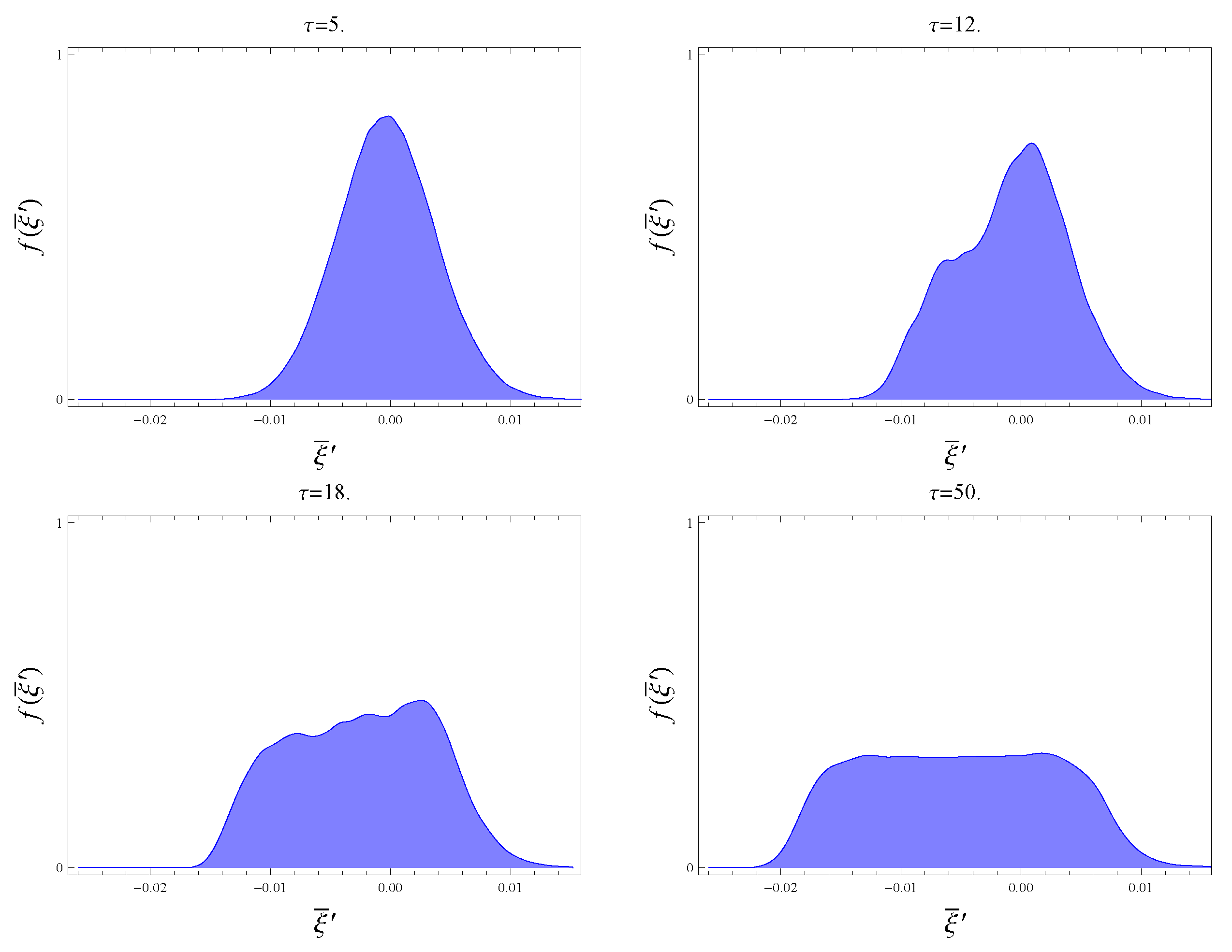
We argued that convective relaxations in the beam-plasma system may occur on intermediate (meso-) time scales and represent a kind of “violent” relaxation phase. This phase completed, the relaxation process proves to be diffusive quasi-linear and in the long run ($t\to +\infty$) leads to the formation of the familiar “plateau” [1,2,5] in the velocity distribution. Mathematically, the relaxation problem for a broad beam is described by a self-consistent system of coupled nonlinear differential equations, Equation (15) and Equation (16), which generalize their quasi-linear relatives by directly taking into account the amplification of the resonance domain through the nonlinear interaction and the communication among the beams. Our analysis is complementary to that of Laval and Pesme in [46], since we consider modifying the convective rather than the diffusion term. Our analysis also applies in a different parameter range; i.e., a regime where the fluctuation spectrum is not arbitrarily broad, in order to allow for non-perturbative beam-coupling.

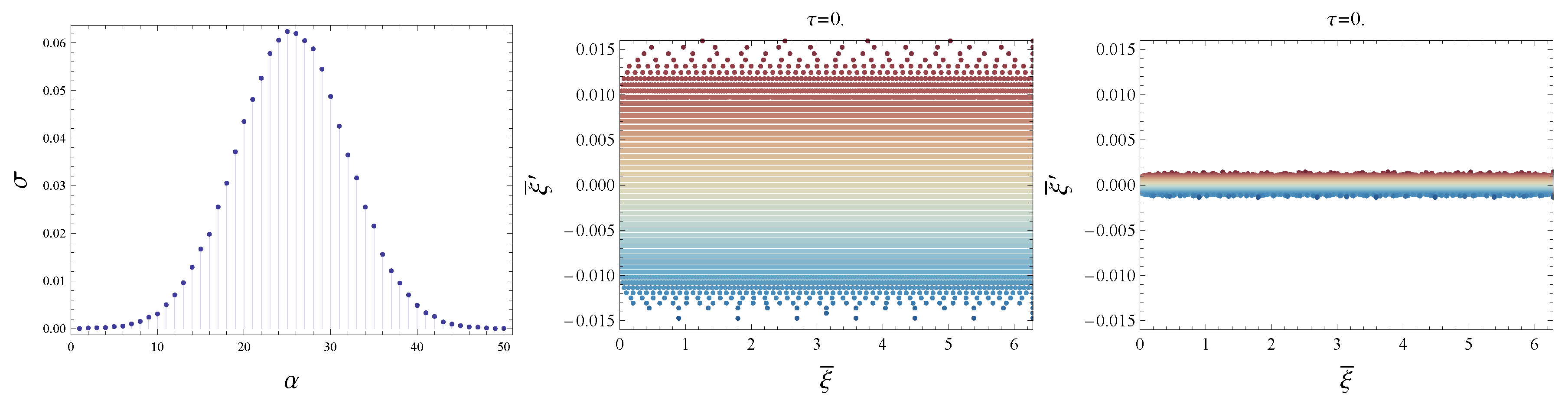
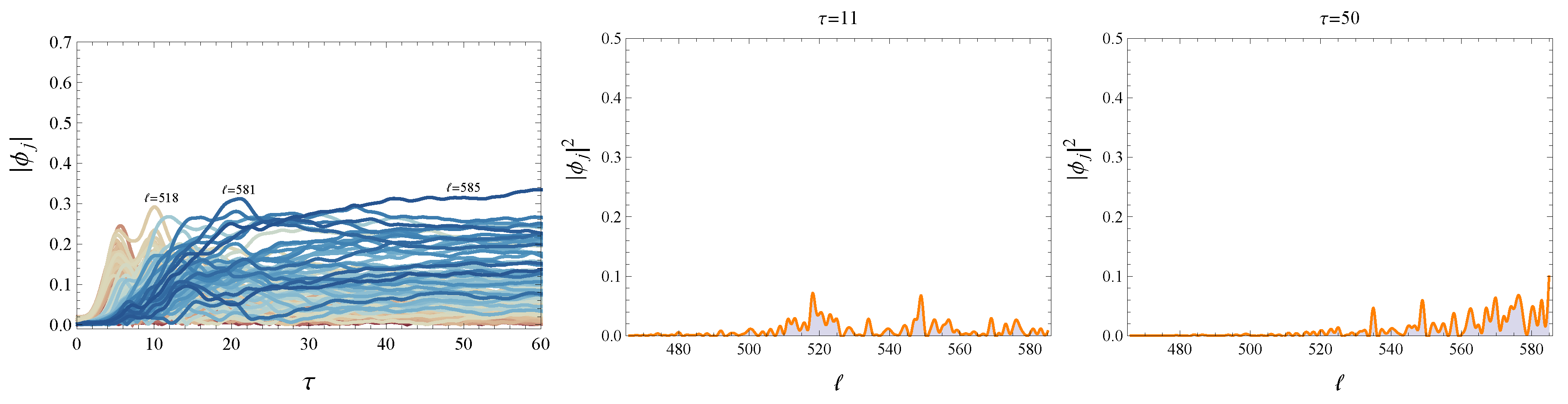
In our numerical studies, we adopt the Hamiltonian formulation of the problem described in [51], where the broad supra-thermal particle beam is discretized as superposition of $n\gg 1$ cold beams self-consistently evolving in the presence of $m\ge n$ modes nearly degenerate with Langmuir waves. The essential element of this analysis is the crucial role played by wave-particle nonlinearity in determining the non-diffusive feature of supra-thermal particle transport, which self-consistently evolves with the fluctuation intensity spectrum. Thus, parameters other than Chirikov play important roles, such as the ratio of wave-particle trapping time to the autocorrelation time (which is related to the ratio of wave-number spectrum width to the Chirikov parameter) and the nonlinearity parameter, straightforwardly related to the former two.

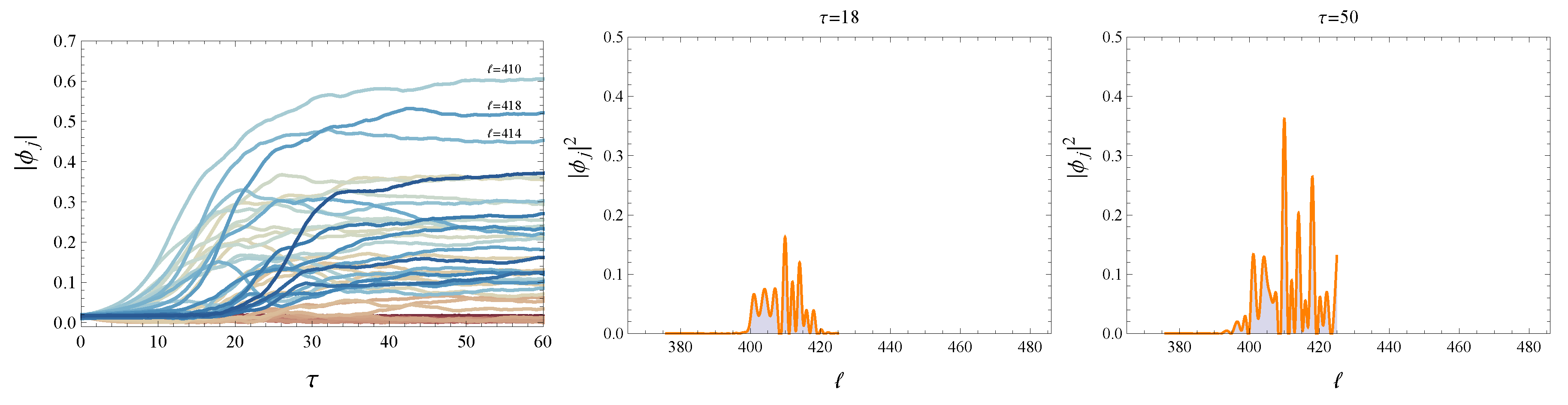
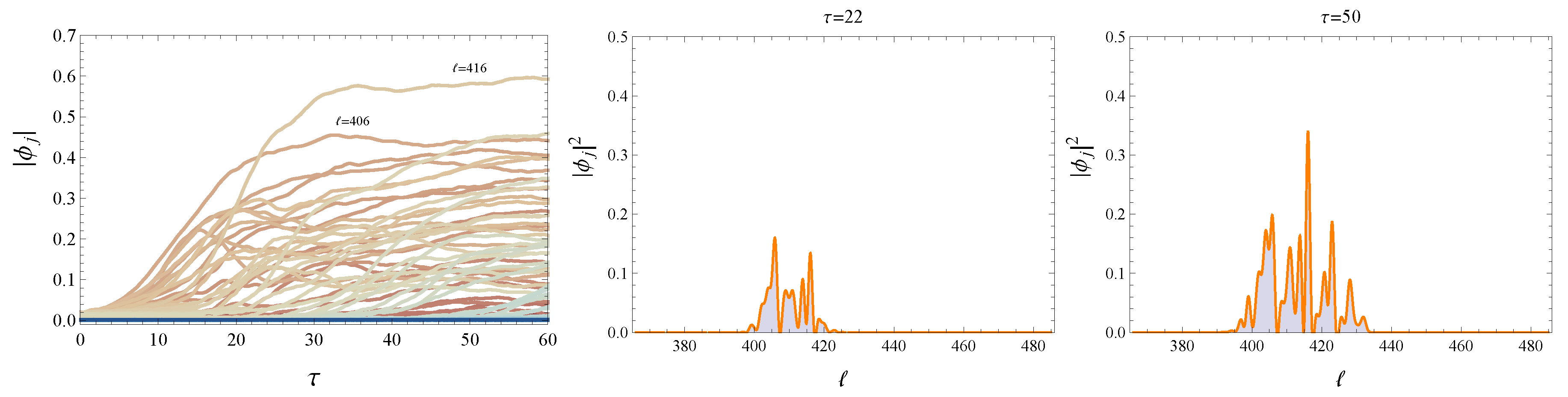
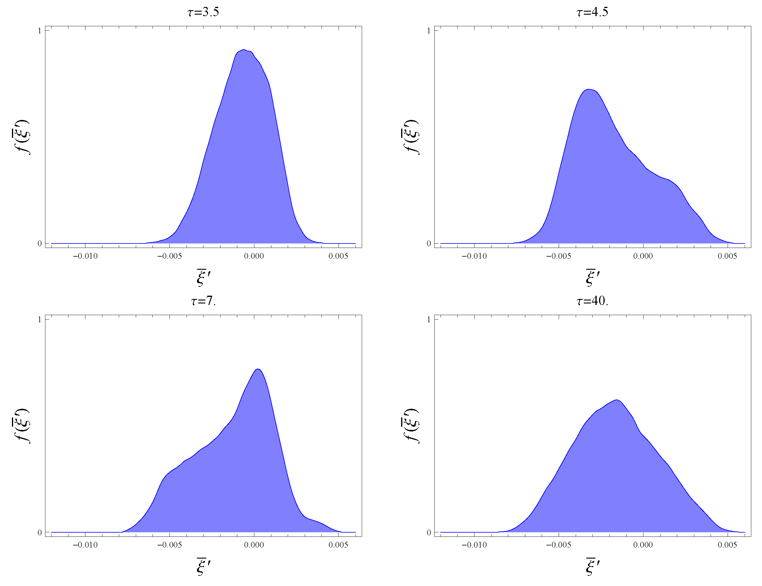
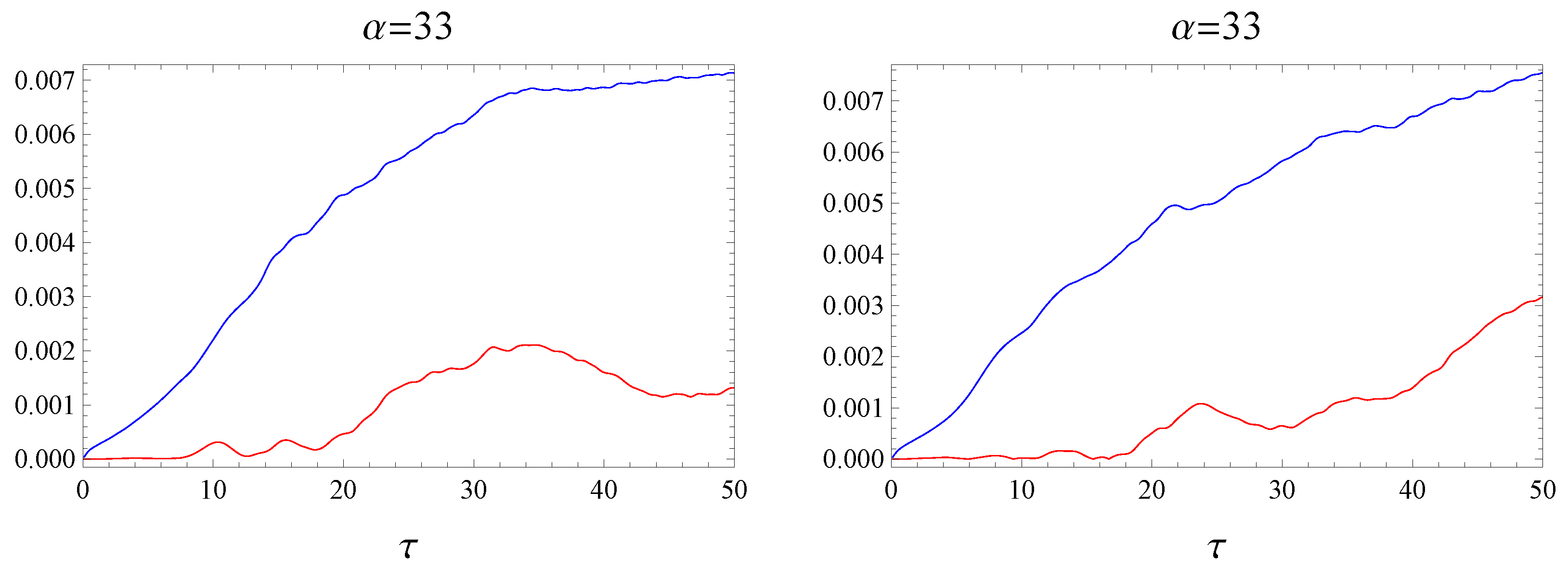
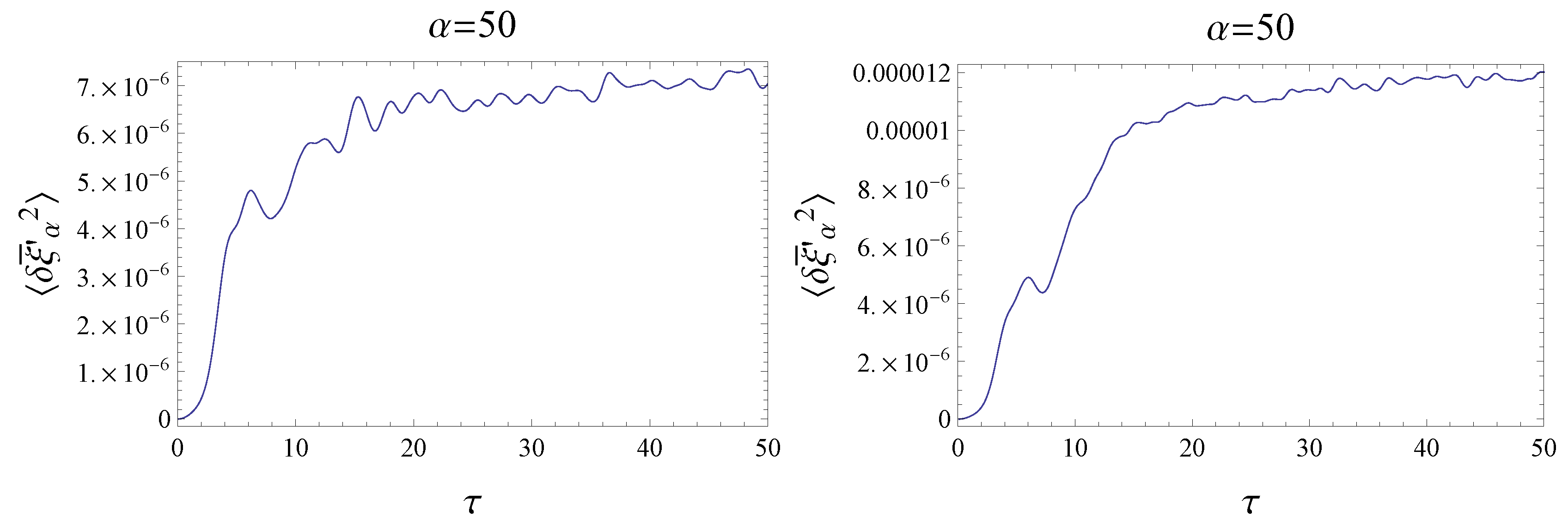
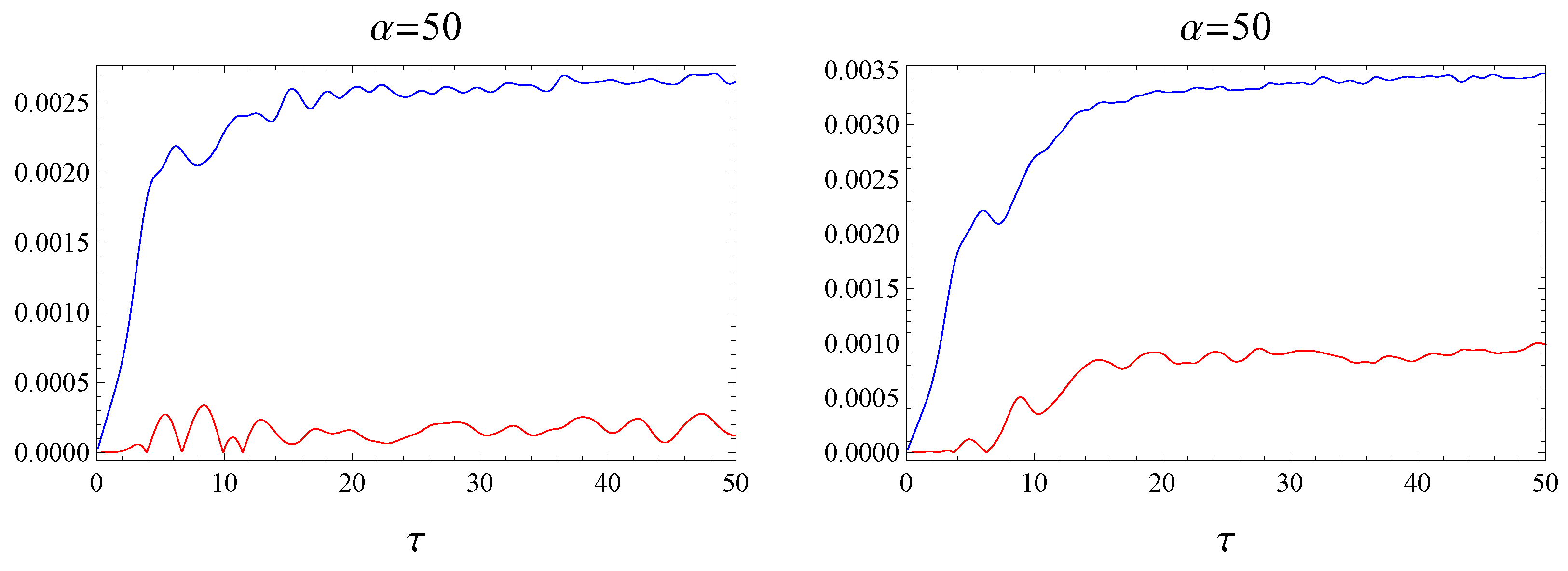
We performed direct computer simulations of the relaxation dynamics in different regimes, i.e., different values of parameters. In this respect, we highlight two cases, namely (i) and (iii), characterized by respectively “broad” and “nearly periodic” (“narrow”) fluctuation spectrum consisting of linearly-unstable modes only; and two corresponding cases, these being (ii) and (iv), in which the modes of the linear stable spectrum have been accounted for, as well. These simulations have elucidated the crucial role played by the linear stable spectrum for transport phenomena through the diffusive and the convective relaxation dynamics.

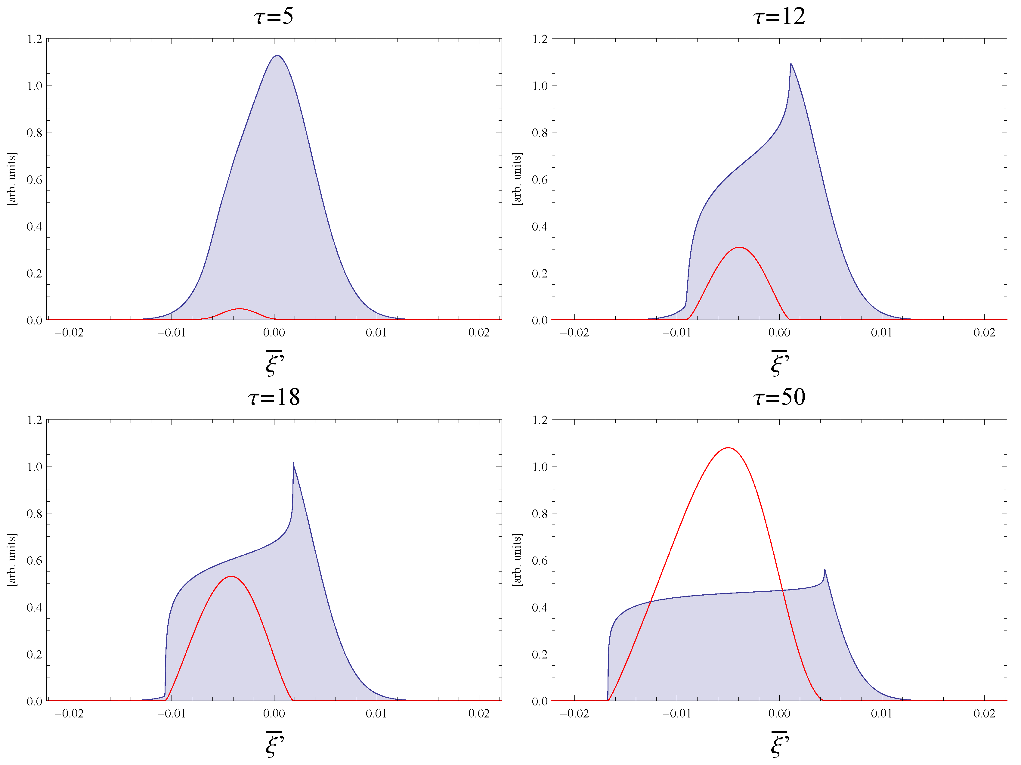
Numerical simulation results for the “narrow” spectrum exhibit the coherent behavior of the spectrum intensity and particle distribution function typical of persistent phase space structures due to wave particle trapping, which suppress convective transport. The plateau in the particle distribution function, in this case, is not formed, unless modes of the linear stable spectrum are accounted for, which not only enhance diffusion, but convection, as well, because of the enhanced de-trapping rate and drag in velocity space.

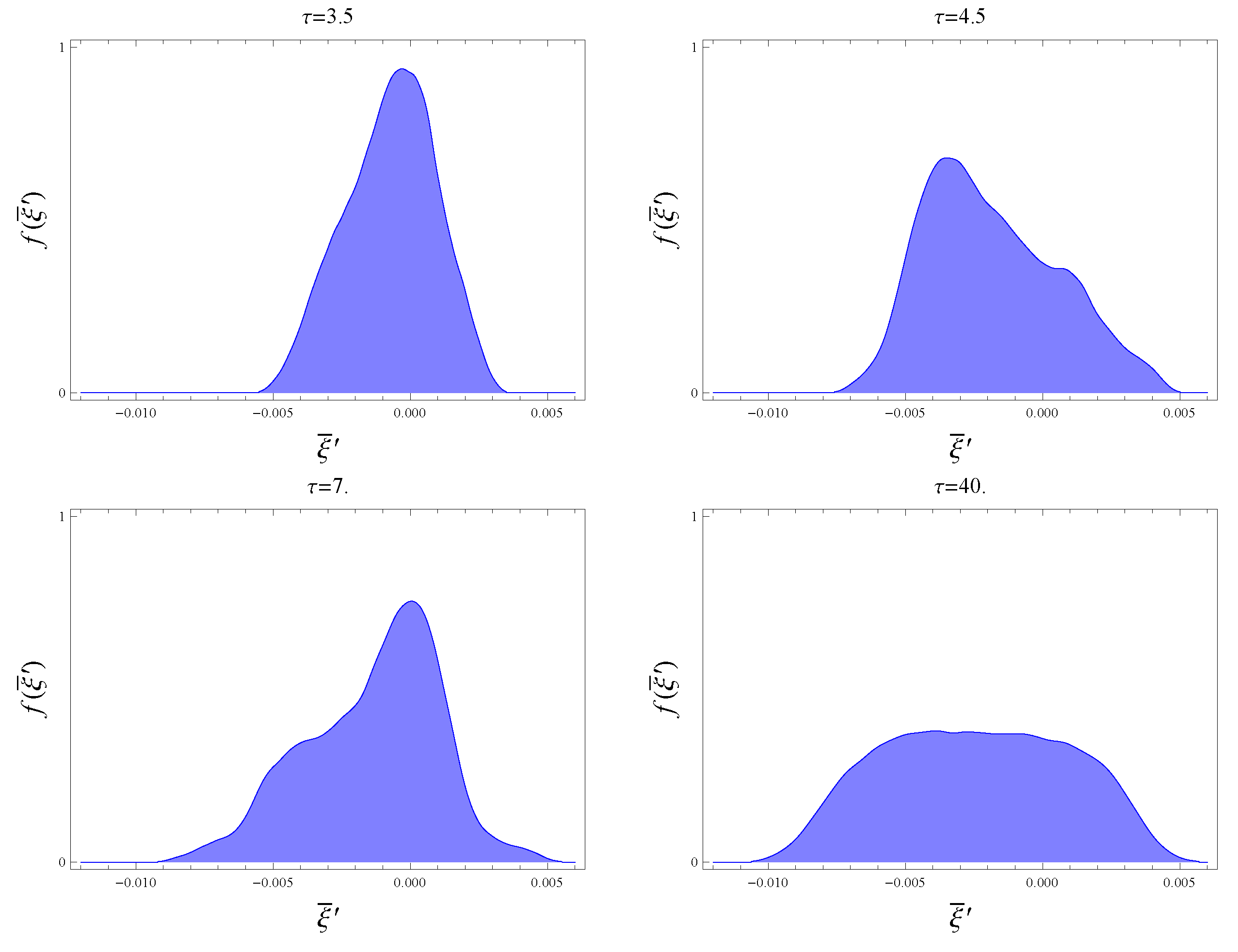
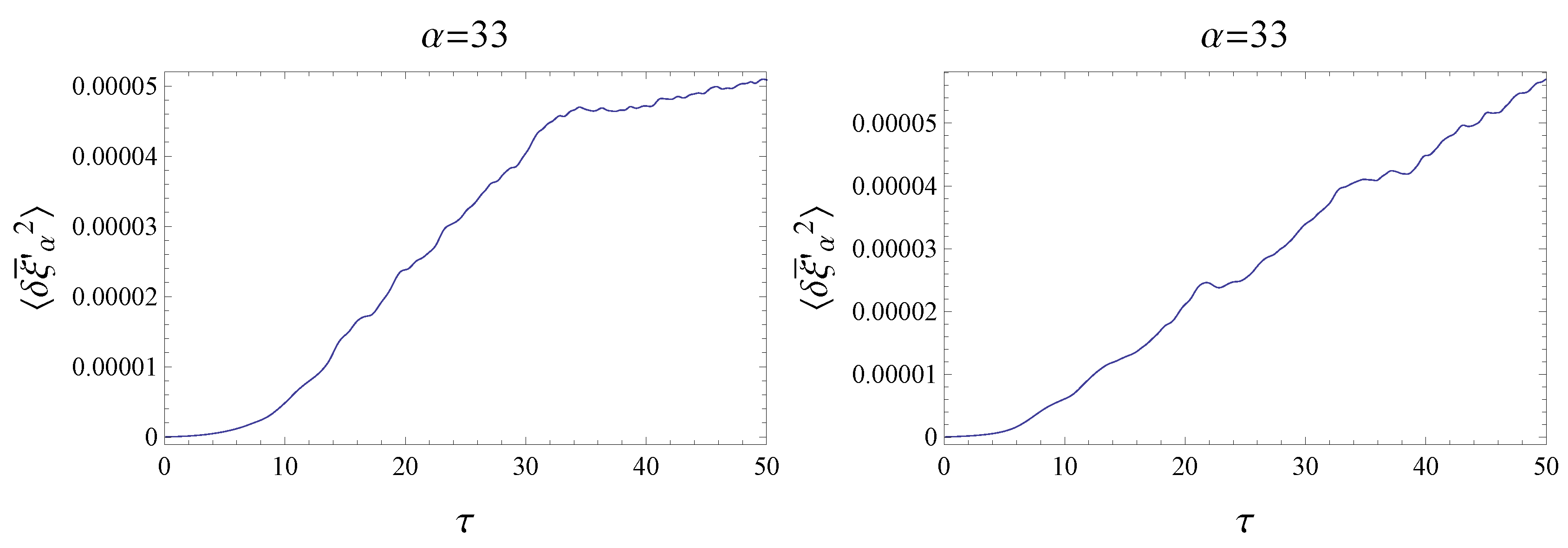
Numerical simulation results for the “broad” spectrum cases, meanwhile, show that a plateau in the distribution function is always formed time asymptotically. Controlling the wave-number spectrum width by including or not the modes of the linear stable spectrum yields behaviors of the diffusion coefficient that are consistent with earlier analyses by Escande et al. [48,49,50]. Further to this, convective transport on temporal and velocity meso-scales is observed even for small nonlinearity parameter. This persistent mixed diffusion-convection relaxation is due to the self-consistent evolution of fluctuation intensity on the same time scale of particle transport, as expected and as demonstrated by an analytical toy-model, whose solution is in good qualitative and quantitative agreement with numerical simulations. This toy-model provides a valuable tool, allowing the identification of respective roles of convection and diffusion in the velocity space relaxation; in particular, elucidating how convection processes are not negligible during the relaxation of a bump-on-tail initial profile, especially during the meso-time scales.

In conclusion, the present study provides understanding and insights into the mixed diffusion-convection relaxation of a broad beam in a cold one-dimensional plasma in the presence of weak Langmuir turbulence of varying spectrum width. In particular, crucial roles are played by wave-particle nonlinearity and the self-consistent evolution of the particle distribution function with the fluctuation intensity spectrum. These results are of general interest, as well as practical importance, in light of their possible implications as a paradigm for Alfvénic fluctuation-induced supra-thermal particle transport in fusion plasmas near marginal stability.

References

1. Vedenov, A.A.; Velikhov, E.P.; Sagdeev, R.Z. Nonlinear oscillations of rarified plasma. Nucl. Fusion 1961, 1, 82–100. [Google Scholar] [CrossRef]
2. Drummond, W.E.; Pines, D. Non-linear Stability of Plasma Oscillations. Nucl. Fusion Suppl. 1962, Suppl. 2, 1049–1057. [Google Scholar]
3. Zaslavsky, G. Statistical Irreversibility in Nonlinear Systems; Nauka: Moscow, Russia, 1970. [Google Scholar]
4. Sagdeev, R.; Zaslavsky, G. Introduction to the Nonlinear Physics. From Pendulum to Turbulence and Chaos; Nauka: Moscow, Russia, 1988. [Google Scholar]
5. Kadomtsev, B. Collective Phenomena in Plasma. 2; Nauka: Moscow, Russia, 1988. [Google Scholar]
6. Bernstein, I.; Greene, J.; Kruskal, M. Exact nonlinear plasma oscillations. Phys. Rev. 1957, 108, 546–550. [Google Scholar] [CrossRef]
7. O’Neil, T.M. Collisionless Damping of Nonlinear Plasma Oscillations. Phys. Fluids 1965, 8, 2255–2262. [Google Scholar] [CrossRef]
8. Mazitov, R.K. Damping of plasma waves. J. App. Mech. Tech. Phys. 1965, 6, 22–25. [Google Scholar] [CrossRef]
9. O’Neil, T.M.; Winfrey, J.; Malmberg, J. Nonlinear Interaction of a Small Cold Beam and a Plasma. Phys. Fluids 1971, 14, 1204–1212. [Google Scholar] [CrossRef]
10. O’Neil, T.M.; Malmberg, J. Transition of the Dispersion Roots from Beam-Type to Landau-Type Solutions. Phys. Fluids 1968, 11, 1754–1760. [Google Scholar] [CrossRef]
11. Shapiro, V. Nonlinear theory of the interaction of a monoenergetic beam with a plasma. Sov. Phys. JEPT 1963, 17, 416–423. [Google Scholar]
12. Onishchenko, I.; Linetskii, A.; Matsiborko, N.; Shapiro, V.; Shevchenko, V. Contribution to the Nonlinear Theory of Excitation of a Monochromatic Plasma Wave by an Electron Beam. JETP Lett. 1970, 12, 281–285. [Google Scholar]
13. Shapiro, V.; Shevchenko, V. Contribution to the Nonlinear Theory of Relaxation of a “Monoenergetic” Beam in a Plasma. Sov. Phys. JEPT 1971, 33, 555–561. [Google Scholar]
14. Thompson, J. Nonlinear Evolution of Collisionless Electron Beam-Plasma Systems. Phys. Fluids 1971, 14, 1532–1541. [Google Scholar] [CrossRef]
15. Levin, M.; Lyubarskiǐ, M.; Onishchenko, I.; Shapiro, V.; Shevchenko, V. Contribution to the Nonlinear Theory of Kinetic Instability of an Electron Beam in Plasma. Sov. Phys. JEPT 1972, 35, 898–901. [Google Scholar]
16. Matsiborko, N.; Onishchenko, I.; Shapiro, V.; Shevchenko, V. On non-linear theory of instability of a mono-energetic electron beam in plasma. Plasma Phys. 1972, 14, 591–600. [Google Scholar] [CrossRef]
17. Dupree, T.H. A Perturbation Theory for Strong Plasma Turbulence. Phys. Fluids 1966, 9, 1773–1782. [Google Scholar] [CrossRef]
18. Berk, H.; Breizman, B. Saturation of a single mode driven by an energetic injected beam. I. Plasma wave problem. Phys. Fluids B 1990, 2, 2226–2234. [Google Scholar] [CrossRef]
19. Berk, H.; Breizman, B. Saturation of a single mode driven by an energetic injected beam. II. Electrostatic “universal” destabilization mechanism. Phys. Fluids B 1990, 2, 2235–2245. [Google Scholar] [CrossRef]
20. Berk, H.; Breizman, B. Saturation of a single mode driven by an energetic injected beam. III. Alfvén wave problem. Phys. Fluids B 1990, 2, 2246–2252. [Google Scholar] [CrossRef]
21. Chen, L.; Zonca, F. Theory of Alfvén waves and energetic particle physics in burning plasmas. Nucl. Fusion 2007, 47, S727–S734. [Google Scholar] [CrossRef]
22. Chen, L.; Zonca, F. On nonlinear physics of shear Alfvén waves. Phys. Plasmas 2013, 20, 055402. [Google Scholar] [CrossRef]
23. Breizman, B.; Sharapov, S. Major minority: Energetic particles in fusion plasmas. Plasma Phys. Control. Fusion 2011, 53, 54001–54039. [Google Scholar] [CrossRef]
24. Chen, L.; Zonca, F. Physics of Alfvén waves and energetic particles in burning plasmas. Rev. Mod. Phys. 2016, 88, 015008. [Google Scholar] [CrossRef]
25. Fasoli, A.; Gormenzano, C.; Berk, H.; Breizman, B.; Briguglio, S.; Darrow, D.; Gorelenkov, N.; Heidbrink, W.; Jaun, A.; Konovalov, S.; et al. Chapter 5: Physics of energetic ions. Nucl. Fusion 2007, 47, S264–S284. [Google Scholar] [CrossRef]
26. Heidbrink, W. Basic physics of Alfvén instabilities driven by energetic particles in toroidally confined plasmas. Phys. Plasmas 2008, 15, 055501. [Google Scholar] [CrossRef]
27. Lauber, P. Super-thermal particles in hot plasmas—Kinetic models, numerical solution strategies, and comparison to tokamak experiments. Phys. Rep. 2013, 533, 33–68. [Google Scholar] [CrossRef]
28. Vlad, G.; Briguglio, S.; Fogaccia, G.; Zonca, F.; Fusco, V.; Wang, X. Electron fishbone simulations in tokamak equilibria using XHMGC. Nucl. Fusion 2013, 53, 083008. [Google Scholar] [CrossRef]
29. Wang, X.; Briguglio, S.; Chen, L.; Di Troia, C.; Fogaccia, G.; Vlad, G.; Zonca, F. An extended hybrid magnetohydrodynamics gyrokinetic model for numerical simulation of shear Alfvén waves in burning plasmas. Phys. Plasmas 2011, 18, 052504. [Google Scholar] [CrossRef]
30. Schneller, M.; Lauber, P.; Bilato, R.; García-Muñoz, M.; Brüdgam, M.; Günter, S.; the ASDEX Upgrade Team. Multi-mode Alfvénic fast particle transport and losses: Numerical versus experimental observation. Nucl. Fusion 2013, 53, 123003. [Google Scholar] [CrossRef]
31. Schneller, M.; Lauber, P.; Brüdgam, M.; Pinches, S.; Günter, S. Double-resonant fast particle-wave interaction. Nucl. Fusion 2012, 52, 103019. [Google Scholar] [CrossRef]
32. Gorelenkov, N.; Pinches, S.; Toi, K. Energetic particle physics in fusion research in preparation for burning plasma experiments. Nucl. Fusion 2014, 54, 125001. [Google Scholar] [CrossRef]
33. Zonca, F.; Chen, L.; Briguglio, S.; Fogaccia, G.; Milovanov, A.; Qiu, Z.; Vlad, G.; Wang, X. Energetic particles and multi-scale dynamics in fusion plasmas. Plasma Phys. Control. Fusion 2015, 57, 014024. [Google Scholar] [CrossRef]
34. Zonca, F.; Chen, L.; Briguglio, S.; Fogaccia, G.; Vlad, G.; Wang, X. Nonlinear dynamics of phase space zonal structures and energetic particle physics in fusion plasmas. New J. Phys. 2015, 17, 013052. [Google Scholar] [CrossRef]
35. Pinches, S.; Chapman, I.; Lauber, P.; Oliver, H.; Sharapov, S.; Shinohara, K.; Tani, K. Energetic ions in ITER plasmas. Phys. Plasmas 2015, 22, 021807. [Google Scholar] [CrossRef]
36. Berk, H.; Breizman, B.; Fitzpatrick, J.; Wong, H. Line broadened quasi-linear burst model [fusion plasma]. Nucl. Fusion 1995, 35, 1661–1668. [Google Scholar] [CrossRef]
37. Berk, H.; Breizman, B.; Fitzpatrick, J.; Pekker, M.; Wong, H.; Wong, K. Nonlinear response of driven systems in weak turbulence theory. Phys. Plasmas 1996, 3, 1827–1838. [Google Scholar] [CrossRef]
38. Ghantous, K.; Gorelenkov, N.; Berk, H.; Heidbrink, W.; van Zeeland, M. 1.5D quasilinear model and its application on beams interacting with Alfvén eigenmodes in DIII-D. Phys. Plasmas 2012, 19, 092511. [Google Scholar] [CrossRef]
39. Ghantous, K.; Berk, H.; Gorelenkov, N. Comparing the line broadened quasilinear model to Vlasov code. Phys. Plasmas 2014, 21, 032119. [Google Scholar] [CrossRef]
40. Lauber, Ph. Local and global kinetic stability analysis of Alfvén eigenmodes in the 15MA ITER scenario. Plasma Phys. Control. Fusion 2015, 57, 054011. [Google Scholar] [CrossRef]
41. Schneller, M.; Lauber, P.; Briguglio, S. Nonlinear energetic particle transport in the presence of multiple Alfvénic waves in ITER. Plasma Phys. Control. Fusion 2016, 58, 014019. [Google Scholar] [CrossRef]
42. Fisch, N. Some Unsolved Challenges In Radio-Frequency Heating and Current Drive. Fusion Sci. Technol. 2014, 65, 79–87. [Google Scholar] [CrossRef]
43. Hay, M.; Schiff, J.; Fisch, N. Maximal energy extraction under discrete diffusive exchange. Phys. Plasmas 2015, 22, 102108. [Google Scholar] [CrossRef]
44. Levy, M.; Wilks, S.; Tabak, M.; Libby, S.; Baring, M. Petawatt laser absorption bounded. Nat. Commun. 2014, 5. [Google Scholar] [CrossRef] [PubMed]
45. Levy, M.; Wilks, S.; Tabak, M.; Baring, M. Conservation laws and conversion efficiency in ultraintense laser-overdense plasma interactions. Phys. Plasmas 2013, 20, 103101. [Google Scholar] [CrossRef]
46. Laval, G.; Pesme, D. Controversies about quasi-linear theory. Plasma Phys. Control. Fusion 1999, 41, A239–A246. [Google Scholar] [CrossRef]
47. Laval, G.; Pesme, D. Self-Consistency Effects in Quasilinear Theory: A Model for Turbulent Trapping. Phys. Rev. Lett. 1984, 53, 270–273. [Google Scholar] [CrossRef]
48. Cary, J.; Doxas, I.; Escande, D.; Verga, A. Enhancement of the velocity diffusion in longitudinal plasma turbulence. Phys. Fluids B 1992, 4. [Google Scholar] [CrossRef]
49. Elskens, Y.; Escande, D.F. Microscopic Dynamics of Plasmas Chaos; IOP Publishing Ltd.: Bristol, UK, 2003. [Google Scholar]
50. Escande, D.; Elskens, Y. Self-consistency vanishes in the plateau regime of the bump-on-tail instability. Plasma Phys. 2008. arXiv:0807.1839. [Google Scholar]
51. Carlevaro, N.; Falessi, M.; Montani, G.; Zonca, F. Nonlinear physics and energetic particle transport features of the beam-plasma instability. J. Plasma Phys. 2015, 81, 495810515. [Google Scholar] [CrossRef]
52. Zaslavsky, G.; Chirikov, B. Stochastic instability of non-linear oscillations. Phys. Uspekhi 1972, 14, 549–568. [Google Scholar] [CrossRef]
53. Zaslavsky, G. Chaos, fractional kinetics, and anomalous transport. Phys. Rep. 2002, 371, 461–580. [Google Scholar] [CrossRef]
54. Chirikov, B. A universal instability of many-dimensional oscillator systems. Phys. Rep. 1979, 52, 263–379. [Google Scholar] [CrossRef]
55. Shapiro, V.D. Nonlinear Theory of the Interaction of a Monoenergetic Beam With a Plasma. Sov. Phys. JETP 1963, 17, 416–423. [Google Scholar]
56. Milovanov, A.; Iomin, A. Localization-delocalization transition on a separatrix system of nonlinear Schrödinger equation with disorder. Europhys. Lett. 2012, 100, 10006. [Google Scholar] [CrossRef]
57. Milovanov, A.; Iomin, A. Topological approximation of the nonlinear Anderson model. Phys. Rev. E 2014, 89, 062921. [Google Scholar] [CrossRef] [PubMed]
58. Metzler, R.; Klafter, J. The restaurant at the end of the random walk: Recent developments in the description of anomalous transport by fractional dynamics. J. Phys. A Math. Gen. 2004, 37, R161–R208. [Google Scholar] [CrossRef]
59. Wax, N. Selected Papers on Noise and Stochastic Processes; Dover: New York, NY, USA, 1954. [Google Scholar]
60. Van Kampen, N.G. Statistic Processes in Physics and Chemistry; North-Holland: Amsterdam, The Netherlands, 1981. [Google Scholar]
61. Risken, H. The Fokker-Planck Equation; Springer-Verlag: Berlin, Geramny, 1989. [Google Scholar]
62. Milovanov, A.; Rasmussen, J. A mixed SOC-turbulence model for nonlocal transport and Lévy-fractional Fokker–Planck equation. Phys. Lett. A 2014, 378, 1492–1500. [Google Scholar] [CrossRef]
63. Milovanov, A.; Rasmussen, J. Self-organized criticality revisited: Non-local transport by turbulent amplification. J. Plasma Phys. 2015, 81, 495810606. [Google Scholar] [CrossRef]
64. Volokitin, A.; Krafft, C. Velocity diffusion in plasma waves excited by electron beams. Plasma Phys. Control. Fusion 2012, 54, 085002. [Google Scholar] [CrossRef]
65. Hasegawa, A. Plasma Instabilities and Nonlinear Effects; Springer-Verlag: Berlin, Geramny, 1975. [Google Scholar]
66. Burgers, J. A mathematical model illustrating the theory of turbulence. Adv. Appl. Mech. 1948, 1, 171–199. [Google Scholar]
67. Ovsiannikov, L.V. Group properties of nonlinear heat equations. Doklady AN SSSR 1959, 125, 492. (In Russian) [Google Scholar]
Figure 1. Left-hand panel: densities of the beams ( σ α ) as a function of the beam index α = 1 , . . . , n . Initial ( τ = 0 ) phase space ( ξ ¯ , ξ ¯ ) for Cases (i), (ii) (central panel) and (iii), (vi) (right-hand panel): each point corresponds to a single charge sheet and different colors denote different beams.
Entropy 18 00143 g001
Figure 2. Case (i). Left-hand panel: temporal evolution of the mode amplitude | ϕ j | ; colors are fixed from blue (largest ) to red (smallest ), and time-asymptotic dominant wave-numbers are indicated. Central and right-hand panels: intensity spectrum at different times.
Entropy 18 00143 g002
Figure 3. Case (i). Evolution of the velocity distribution function f ( ξ ¯ ) (in arbitrary units), shown at different times.
Entropy 18 00143 g003
Figure 4. Case (ii). Left-hand panel: temporal evolution of | ϕ j | . Central and right-hand panels: intensity spectrum at different times.
Entropy 18 00143 g004
Figure 5. Case (ii). Evolution of the velocity distribution function.
Entropy 18 00143 g005
Figure 6. Case (iii). Left-hand panel: temporal evolution of | ϕ j | . Central and right-hand panels: intensity spectrum at different times.
Entropy 18 00143 g006
Figure 7. Case (iii). Evolution of the velocity distribution function.
Entropy 18 00143 g007
Figure 8. Case (iv). Left-hand panel: temporal evolution of | ϕ j | . Central and right-hand panels: intensity spectrum at different times.
Entropy 18 00143 g008
Figure 9. Case (iv). Evolution of the velocity distribution function.
Entropy 18 00143 g009
Figure 10. Temporal evolution of δ ξ ¯ 33 2 ( τ ) for test particles initialized at ξ ¯ 33 i ( 0 ) (near the central beam): in the left-hand panel for Case (i) and in the right-hand panel for Case (ii). The linear (diffusive) time behavior is evident.
Entropy 18 00143 g010
Figure 11. Overlap of the temporal evolution of δ ξ ¯ 33 2 (blue line) and ξ ¯ 33 ξ ¯ 33 ( 0 ) (red line), for test particles initialized at ξ ¯ 33 i ( 0 ) . Case (i) in the left-hand panel and Case (ii) in the right-hand panel.
Entropy 18 00143 g011
Figure 12. Time evolution of of δ ξ ¯ 50 2 ( τ ) for tracers initialized at ξ ¯ 50 i ( 0 ) : in the left-hand panel for Case (iii) and in the right-hand panel for Case (iv).
Entropy 18 00143 g012
Figure 13. Overlap of the evolution of δ ξ ¯ 50 2 (blue line) and ξ ¯ ξ ¯ 50 ( 0 ) (red line), for test particles initialized at ξ ¯ 50 i ( 0 ) . Case (iii) in the left-hand panel and Case (iv) in the right-hand panel.
Entropy 18 00143 g013
Figure 14. Evolution of the velocity distribution function G 0 (blue filled line) and the spectral density E (red line) as a function of the normalized velocity ξ ¯ at different stages of the evolution of Figure 3.
Entropy 18 00143 g014
Figure 15. Plot of E numerically estimated from Equation (31) (blue line) and the theoretical values of E calculated from Equation (34) (red line), versus the normalized velocity ξ ¯ at a fixed time τ = 40 .
Entropy 18 00143 g015