Multi-Level Formation of Complex Software Systems

Abstract

We present a multi-level formation model for complex software systems. The previous works extract the software systems to software networks for further studies, but usually investigate the software networks at the class level. In contrast to these works, our treatment of software systems as multi-level networks is more realistic. In particular, the software networks are organized by three levels of granularity, which represents the modularity and hierarchy in the formation process of real-world software systems. More importantly, simulations based on this model have generated more realistic structural properties of software networks, such as power-law, clustering and modularization. On the basis of this model, how the structure of software systems effects software design principles is then explored, and it could be helpful for understanding software evolution and software engineering practices.

1. Introduction

Many systems in nature and society reveal network organizations. These networks, such as biological protein networks [1], science collaborations [2,3], social networks [4] and the Internet [5], have been found to represent some attributes, such as scale free, small world, etc. These discoveries emerge from the science of complex networks. Recent studies have revealed that object-oriented software systems share some structural attributes with these complex networks. Specifically, the networks of software systems are characterized by a scale-free degree distribution [6,7,8,9,10], a small-world structure (short average path length and high clustering) [11,12] and some other features [13,14,15,16,17,18]. This therefore raises the study of software networks in recent years.

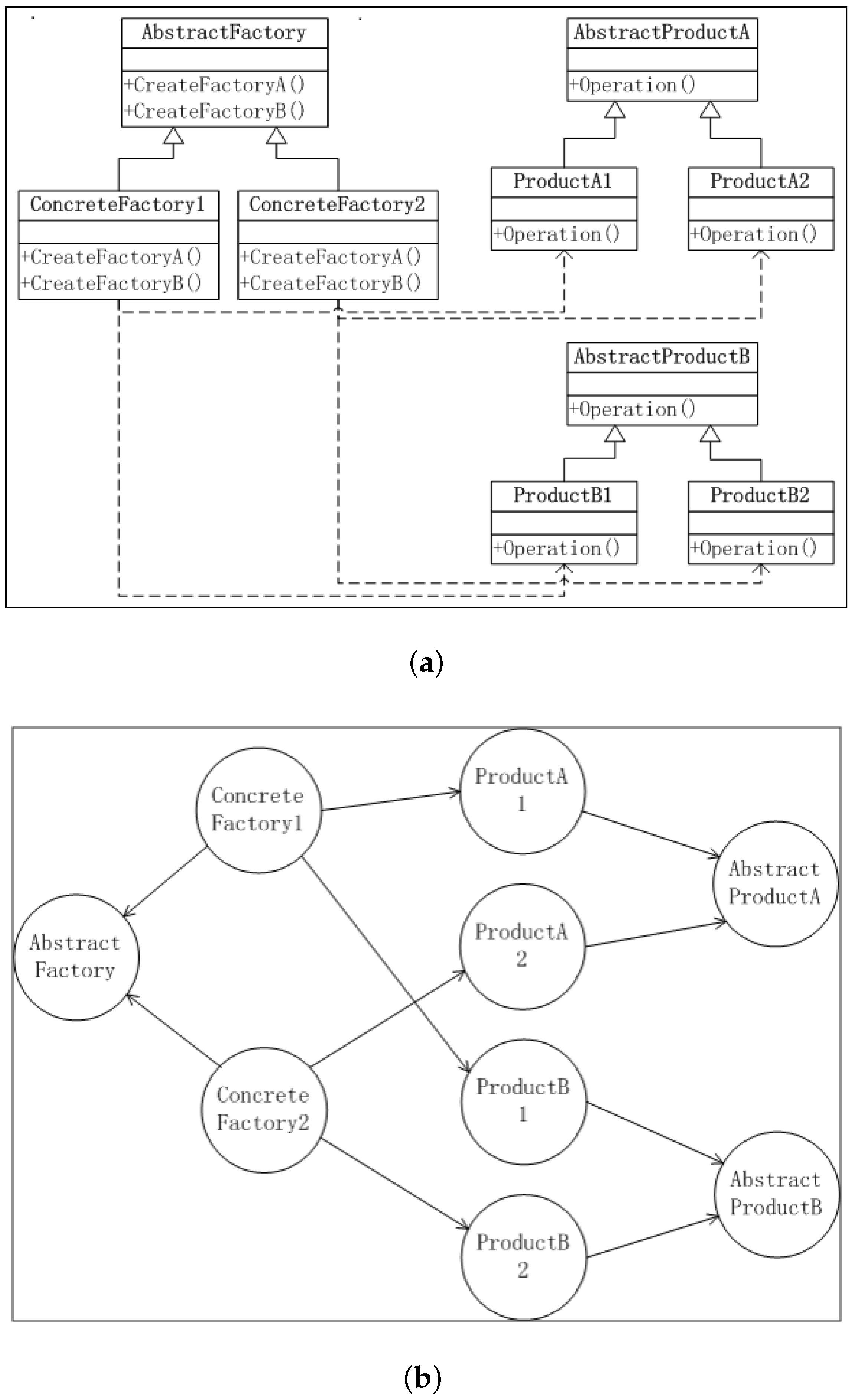
Software systems consist of many interacting units at some levels of granularity, such as methods, classes and subsystems [19]. Additionally, the collaborations of these units in a software system can be therefore extracted and defined as a software network. Figure 1 shows a simple example of the extraction from a software system to a software network, in which the classes in the left figure are nodes and the collaborations of such nodes are edges. For the software systems with a more complex structure, the corresponding software networks are organized to be highly functional, modularized [19] and evolvable [15]. This therefore brings some further studies on software networks, such as community detection [20,21], quality assessment [10], important unit identification [22], bug classification [23] and developer social collaboration [24,25], which are helpful to various phases in software engineering practices.

During the whole production process of a software project, the design phase is the most critical stage because the structure of the units at different levels and the collaborations of such units are explicitly described in this process. These collaborations enable the detailed functional tasks to be integrated by many reusable basic units in a modular and hierarchical fashion [11]. However, some other crucial and persistent actions in the lifecycle of software systems, such as software maintenance, refactoring and adaptation, cannot be carried out in the task of software design, but lie in the formation of software systems. The goal of a software project is not only building up a software system to satisfy the functional requirement, but also making the software systems convenient and economical to upgrade to new versions. Thus, it makes the evolution of software networks an increasingly important issue.

However, while active research has been undertaken and many solid results have been obtained for understanding the formation mechanisms of these natural and man-made systems, the same work has been only very sparsely performed on software systems, and little has been achieved about the cause-effect relationship between software engineering practices and the structure of these systems.

From the view of software engineering, software evolution is a process of meeting the dynamical requirement changes of the users. From the view of entropy, software evolution is a process of network structural change from chaos to order. As a kind of typical open system, the structure of software systems is dynamically changing under an external driving force, and the changing reveals the status of system designing and coding [26]. Therefore, studying how the software systems evolve can help in a number of areas, including software testing, software maintenance and program comprehension [27] and further to evaluate the system robustness and its ability to tolerate changes [28].

Based on various of empirical studies [15,29,30,31,32,33,34,35], a few models of software network evolution, which describe the evolutionary mechanism from different perspectives, have been proposed. The models reported in [11,36,37,38,39] are respectively based on refactoring processes, node aging affect, weighted network and software patterns. These models perform well in some aspects of software network evolution, and the work can forecast the evolution trends based on the model [39]. However, they do not explicitly include some important qualities of software networks, e.g., modularity and hierarchy. In reality, however, software systems are characterized by high modularity [11,21,40], which corresponds to the important principle of high cohesion and low coupling in software design [41], and the practice of software architecture design assures that software networks are hierarchical and multigranular by nature [13,42,43,44]. In addition, most of these models adopt a undirected graph, which is appropriate for some types of networks, such as the Internet and social networks, to represent software networks. However, software networks are directed because dependent relations between basic units in software systems are unidirectional, and the direction is designated when the node is added to the network [45].

Here, we stress another salient fact about the evolution of software systems, which is missing in most of the existing models. With respect to evolution, these systems lie somewhere between natural systems, which are characterized by a bottom-up self-organizing process, and conventional engineering systems, whose upgrades are governed by a top-down central design, because the work of software design is a social work in which many designers and developers are working together to carry out the task [24]. On the one hand, software architecture supports more autonomous attachments in comparison to other types of architecture, because objects are loosely coupled, and adding or removing non-core objects usually does not significantly affect the rest of the system. On the other hand, in enhancing software systems, some issues should be taken into consideration, such as reuse, maintenance, performance and optimization. They all call for a comprehensive viewpoint and overall design.

In view of the current situation discussed above, we aim at more accurately understanding the general mechanism that governs the evolution of software systems and exploring the cause-effect relationship between a variety of software development principles and the structure of software systems. To accomplish this goal, we have developed a multi-level model of software evolution, which represents software systems as directed networks and adopts a modular binding process for new component attachments.

The rest of this paper is structured as follows. In Section 2, we describe the multi-level model, in terms of structure and the evolutionary mechanism. Section 3 exhibits simulation results based on the model and compares them to empirical data. In Section 4, we explore the implications of various software design principles for the structure of software systems. Section 5 concludes this work and presents possible future works.

2. The Multi-Level Model of Software Evolution

2.1. Levels of Software Systems

Software systems are multi-level systems by nature. In this work, we consider three typical levels of software systems, which are outlined in

Table 1. Levels of a software network and their elements.

Level	Elements
I	classes, interfaces, structs
II	motifs, patterns, libraries, frameworks
III	packages, subsystems, components

.

We represent a software system on each level as a directed graph $G=\{V,E\}$. Here, V is a set of elements that are termed nodes; E is a set of ordered node pairs, each of which implies that the first node depends on the second one, and this relation of dependence is depicted as an edge that leaves the first and enters the second node. The sets of elements on Levels I, II and III are denoted respectively by $\{v_{i,j,k}^{\mathrm{I}}\}$, $\{v_{i,j}^{\mathrm{II}}\}$, and $\{v_i^{\mathrm{III}}\}$. Therefore, the element $v_{i,j,k}^{\mathrm{I}}$ on Level I is the i-th element of $v_{j,k}^{\mathrm{II}}$ on Level II, and $v_{j,k}^{\mathrm{II}}$ in turn is the j-th element of $v_k^{\mathrm{III}}$ on Level III, which is the k-th element on this largest scale.

In the following part of this section, we will give more detailed descriptions of the three levels.

2.1.1. Level I

In software systems, some basic units, such as classes, encapsulate fundamental functions for constructing more complex and application-specific elements on larger scales. We term the scale corresponding to these units Level I.

Collaborations among these basic elements form the microstructure of a software system. Specifically, there are two types of dependencies between these elements: inheritance implies a relationship of “is a”, and association corresponds to “has a”. We follow the convention of software engineering in depicting a dependence: an edge is directed from Element B to Element A if B, in its definition, makes reference to (or is dependent on) A. In our analysis, repeated links are not considered.

2.1.2. Level II

In software practices, some combinations of classes or other basic units appear with much higher frequencies than would be expected by pure chance [42], although some do not work in modern software engineering [46]. These patterns, such as motifs, are usually composed of a few basic (Level I) elements. They are general repeatable solutions to some commonly-occurring problems in software design or have been reused over time in different systems to perform various information processing functions. Being building blocks of more complex software structures, they constitute a natural level between the basic units, such as classes, and the entire software system. We name it Level II.

In reality, Level II elements are usually composed of three or four Level I elements. An important fact is that Level II elements with few internal links appear more frequently than those with many internal connections [42]. The high probability of these sparse graphs is caused by the software engineering principle that coupling should be minimized [47]. The most commonly-used Level II elements are displayed in Figure 2.

2.1.3. Level III

Component-based software engineering has become a widely-adopted reuse-oriented approach to software development, and software evolution usually involves adding new components to existing systems. In comparison with single classes that can be used only if the detailed knowledge about them is known, components are more encapsulated, abstract and easy to use.

In our model, components lie on Level III. They contain different numbers of Level II elements and eventually different numbers of Level III elements, conforming to the empirical fact that the sizes of components vary from a few objects to whole applications.

2.2. The Mechanism of Software Evolution

Empirically, software networks keep growing in response to changing conditions and new requirements, in line with the empirical studies on a large number of real software systems [48,49]. Consequently, new functional modules are continually added into software systems, and these elements are much more than those that are removed. The work in [44] further reported that, in real software systems, both elements and edges tend to grow on different levels simultaneously.

There is an empirical fact that, although newly-added elements have different functions and sizes, the numbers of the edges between them and the existing elements are quite close to one another. For simplicity, we consider these numbers as equal and treat them as a constant that is denoted by $R_e$. Its value can be obtained by averaging the corresponding values of the elements in different systems.

There are a few parameters in our model: reuse probability Γ, common to elements on all three levels, expresses the general degree of reuse; coupling ratio Λ is the ratio of the number of the edges that connect all of the Level II elements within the same Level III element to all of the Level II edges related to the Level III element; the total size of the whole software system at the end of the evolution $N_{\mathrm{I}}$, in terms of the number of Level I elements; and the minimum size $N_{\mathrm{I},min}^{\mathrm{III}}$ and maximum size $N_{\mathrm{I},max}^{\mathrm{III}}$ of the Level III elements, in terms of the number of Level I elements.

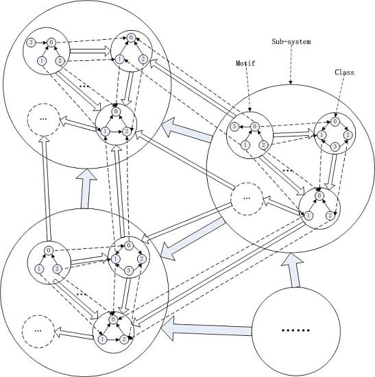
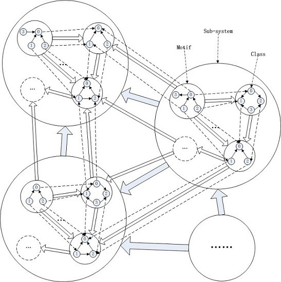
The mechanism of evolution can be described as the following algorithm and correspondingly depicted as Figure 3. One should note that an edge between two Level II elements is established because two Level I elements separately belonging to the two Level II elements are connected. Likewise, an edge between two Level III elements is established because two Level II elements separately belonging to the two Level II elements are connected.

Step 1

Determine the values of $N_{\mathrm{I}}$, $N_{\mathrm{I},min}^{\mathrm{III}}$, $N_{\mathrm{I},max}^{\mathrm{III}}$, Λ and Γ.

Step 2

Create a new Level III element $v_k^{\mathrm{III}}$ with a random size $n_k^{\mathrm{III}}$.

Step 2.1

In $v_k^{\mathrm{III}}$, create a new Level II element $v_{j,k}^{\mathrm{II}}$ of a random type.

Step 2.2

Link $v_{j,k}^{\mathrm{II}}$ to an existing Level II element in $v_k^{\mathrm{III}}$ with directions depending on Γ. The existing element is selected by probability $P_{\mathrm{in}}\left(D_{\mathrm{in}}\right)$ or $P_{\mathrm{out}}\left(D_{\mathrm{out}}\right)$.

Step 2.3

With the determined direction, link $E_{\mathrm{I}}^{\mathrm{II}{,}^{\prime }}$ (see Section 2.2.5) pairs of Level I elements between $v_{j,k}^{\mathrm{II}}$ and the existing element.

Step 2.4

If $v_{j,k}^{\mathrm{II}}$ has linked to $R_e(1-\mathsf{\Lambda })$ existing Level II elements in $v_k^{\mathrm{III}}$, continue; else, go to Step 2.2.

Step 2.5

If the number of Level III elements in $v_k^{\mathrm{III}}$ reaches $n_k^{\mathrm{III}}$, go to Step 3; else, go to Step 2.1.

Step 3

Attach $v_k^{\mathrm{III}}$ to an existing Level III element with directions depending on Γ. It is selected with probability $P_{\mathrm{in}}\left(D_{\mathrm{in}}\right)$ or $P_{\mathrm{out}}\left(D_{\mathrm{out}}\right)$.

Step 3.1

Select a Level II element $v_{j,k}^{\mathrm{II}}$ from $v_k^{\mathrm{III}}$, and link to an existing Level II element in the existing Level III element by probability $P_{\mathrm{in}}\left(D_{\mathrm{in}}\right)$ or $P_{\mathrm{out}}\left(D_{\mathrm{out}}\right)$.

Step 3.2

With the determined direction, link $E_{\mathrm{I}}^{\mathrm{II}{,}^{\prime }}$ pairs of Level I elements between $v_{j,k}^{\mathrm{II}}$ and the existing Level II element.

Step 3.3

If $R_e\mathsf{\Lambda }{n}_k^{\mathrm{III}}$ (see Section 2.2.4) pairs of Level II elements have been linked between $v_k^{\mathrm{III}}$ and the existing Level III element, go to Step 4; else, go to Step 3.1.

Step 4

If the number of Level III elements in all Level I elements reaches $N_{\mathrm{I}}$, go to Step 5; else, go to Step 2.

Step 5

End the process.

In the rest of this section, we present a more detailed explanation of the mechanism.

2.2.1. Direction of Attachment

The direction of the edges is determined in the following manner: (1) it will reuse an existing module and establish an outgoing edge with reuse probability Γ$(0\le \mathsf{\Gamma }\le 1)$; (2) it depends on an existing module and receives an incoming edge with probability $1-\mathsf{\Gamma }$. Γ is positively related to the general degree of reuse. We adopt a great value for Γ on account of the fact that, in the software development practice, there is a strong inclination to reuse.

2.2.2. Probability of Attachment

In software engineering practices, the elements with high incoming dependencies usually have a simple structure and perform some fundamental functions. These elements could be reused for a greater probability to be reused and receive incoming links. In contrast, the elements with more outgoing dependencies, such as modules of user interfaces, usually represent a more complex structure within the elements. They are more likely to depend on other elements and establish outgoing links. Due to their complexity, it is dangerous for the system if these elements are dependent on other elements.

Consequently, elements with larger in-degrees are more likely to receive incoming edges, while those with larger out-degrees are more likely to link to other elements with outgoing edges [45]. Therefore, we can consider that the probability that an element receives an incoming edge $P_{\mathrm{in}}\left(D_{\mathrm{in}}\right)$ is proportional to its in-degree $D_{\mathrm{in}}$, and that with which elements establish an outgoing edge $P_{\mathrm{out}}\left(D_{\mathrm{out}}\right)$ is proportional to its out-degree $D_{\mathrm{out}}$, i.e.,

$$\begin{array}{c}\hfill P_{\mathrm{in}}\left(D_{\mathrm{in}}\right)\sim D_{\mathrm{in}},\end{array}$$

and:

$$\begin{array}{c}\hfill P_{\mathrm{out}}\left(D_{\mathrm{out}}\right)\sim D_{\mathrm{out}}.\end{array}$$

2.2.3. Level III

We assume that $N_{\mathrm{I}}$ Level I elements will be added to the existing network. New Level III elements $\{v_k^{\mathrm{III}}\}$ with a random number of Level I elements will be generated and added, one by one, to the existing network, until the total number of Level I elements of the whole system reaches $N_{\mathrm{I}}$. The size of each Level III element $v_k^{\mathrm{III}}$ is between $N_{\mathrm{I},min}^{\mathrm{III}}$ and $N_{\mathrm{I},max}^{\mathrm{III}}$, and there are $R_e$ edges that connect this element to other existing Level III elements.

2.2.4. Level II

The edges of each Level II element are of two types: internal edges connecting it to other elements in the same Level III element and edges that link to elements in other Level III elements. We use the parameter named coupling ratio Λ for the proportion of the second type of edges. A high (low) value of Λ therefore corresponds to high coupling and low cohesion (low coupling and high cohesion).

In the evolutionary process, when a new Level II element $v_{j,k}^{\mathrm{II}}$ is added into a Level III element $v_k^{\mathrm{III}}$, $R_e\mathsf{\Lambda }$ internal edges form between $v_{j,k}^{\mathrm{II}}$ and other Level II elements in $v_k^{\mathrm{III}}$. Since $v_k^{\mathrm{III}}$ contains $N_{\mathrm{II}}^{\mathrm{III}}$ Level II elements, there will be $N_{\mathrm{II}}^{\mathrm{III}}{R}_e(1-\mathsf{\Lambda })$ internal edges and $N_{\mathrm{II}}^{\mathrm{III}}{R}_e\mathsf{\Lambda }$ edges connecting different Level II elements within $v_k^{\mathrm{III}}$.

When an edge is added between the new Level III element $v_k^{\mathrm{III}}$ and an existing Level III element, $R_e{N}_{\mathrm{II}}^{\mathrm{III}}\mathsf{\Lambda }$ pairs of Level II elements between the two Level III elements are linked through Level II edges and with the same direction as the Level III edge. The probabilities for each pair of Level II elements to get an incoming edge and an outgoing edge are $P_{\mathrm{in}}\left(D_{\mathrm{in}}\right)$ and $P_{\mathrm{out}}\left(D_{\mathrm{out}}\right)$, respectively.

2.2.5. Level I

Empirically, a Level II element is composed of three or four Level I elements of 14 types (see Figure 2). When a Level II element is generated, the number of internal Level I edges depends on the type of the Level II element. For simplicity, we assume that the 14 types of Level I elements appear in every Level II element with an equal probability. Consequently, we can get the average number of Level I elements ${\overline{N}}_{\mathrm{I}}^{\mathrm{II}}=(1/n){\sum }_{j=1}^n{N}_{\mathrm{I},j}^{\mathrm{II}}$ and the average number of Level I edges ${\overline{E}}_{\mathrm{I}}^{\mathrm{II}}=(1/n){\sum }_{j=1}^n{E}_{\mathrm{I},j}^{\mathrm{II}}$.

We assume that there are $N_{\mathrm{II}}^{\mathrm{III}}$ Level II elements in the current Level III element, and $E_{\mathrm{I}}^{\mathrm{II}{,}^{\prime }}$ Level I level interacting edges are added when a Level II level edge is added. The total number of Level I edges is equal to the sum of the total number of internal edges and the total number of interacting edges:

$$\begin{array}{c}\hfill N_{\mathrm{II}}^{\mathrm{III}}{\overline{N}}_{\mathrm{I}}^{\mathrm{II}}{R}_e=N_{\mathrm{II}}^{\mathrm{III}}{\overline{E}}_I^{\mathrm{II}}+E_I^{\mathrm{II}{,}^{\prime }}{N}_{\mathrm{II}}^{\mathrm{III}}{R}_e,\end{array}$$

then we have:

$$\begin{array}{c}\hfill E_{\mathrm{I}}^{\mathrm{II}{,}^{\prime }}={\overline{N}}_{\mathrm{I}}^{\mathrm{II}}-\frac{{\overline{E}}_{\mathrm{I}}^{\mathrm{II}}}{R_e}.\end{array}$$

We can therefore simply consider that each Level II element contains ${\overline{N}}_{\mathrm{I}}^{\mathrm{II}}$ Level II elements and ${\overline{E}}_{\mathrm{I}}^{\mathrm{II}}$ Level II edges. When an edge is added between the new Level II element $v_{j,k}^{\mathrm{II}}$ and an existing Level II element, $E_{\mathrm{I}}^{\mathrm{II}{,}^{\prime }}$ pairs of edges between the two elements are linked by Level I level edges and with the same direction as that of the Level II level edge. The selected probabilities for each pair of elements to get the incoming edge and the outgoing edge are $P_{\mathrm{in}}\left(D_{\mathrm{in}}\right)$ and $P_{\mathrm{out}}\left(D_{\mathrm{out}}\right)$, respectively.

3. Simulation Results

In this section, some essential results of simulations based on our multi-level model are displayed. The simulations were undertaken with respect to the structural properties of our simulated software network. We explored the influences of four parameters: coupling ratio Λ, reuse probability Γ and the minimum size $N_{\mathrm{I},min}^{\mathrm{III}}$ and the maximum size $N_{\mathrm{I},max}^{\mathrm{III}}$ of the Level III elements. The values for $E_{\mathrm{I}}^{\mathrm{II}{,}^{\prime }}$ and $R_e$ are adopted as, respectively, the average values of their corresponding empirical observations.

For validating our modeling, the simulation results are compared to data presented in some real-world software systems, such as Blender, Doxygen, Eclipse, etc. More importantly, these simulations enable more comprehensive understanding of the evolutionary mechanisms under study.

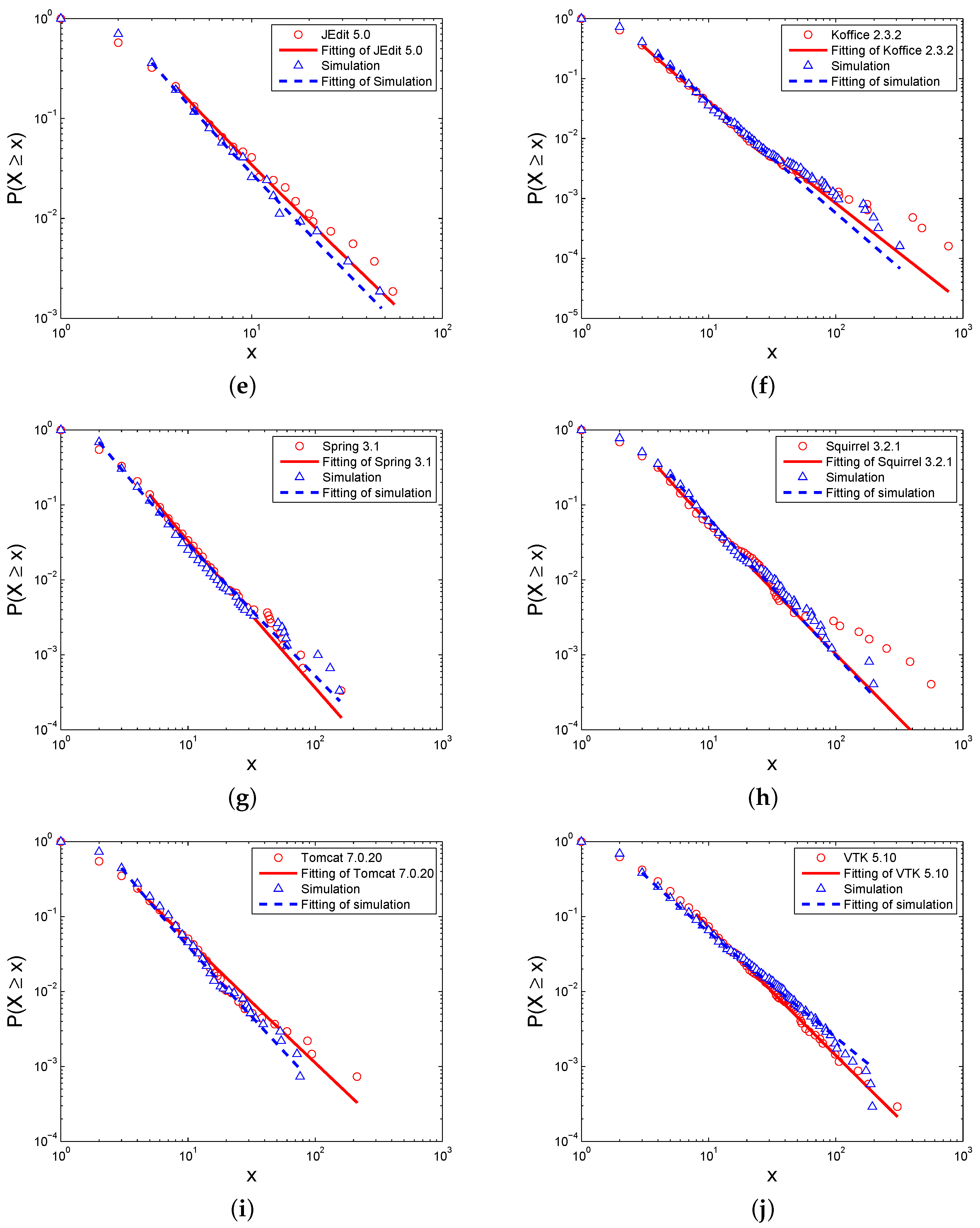
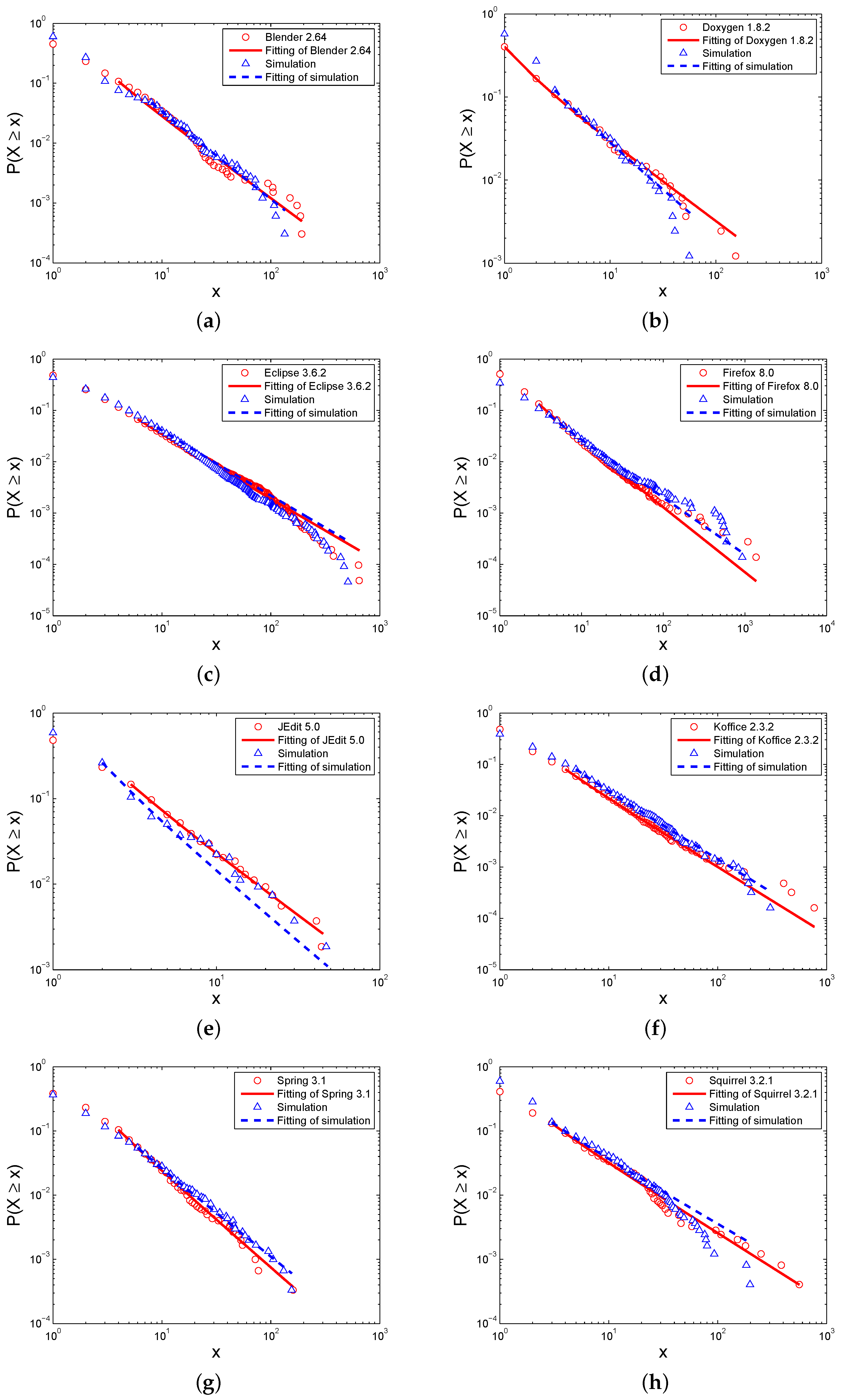
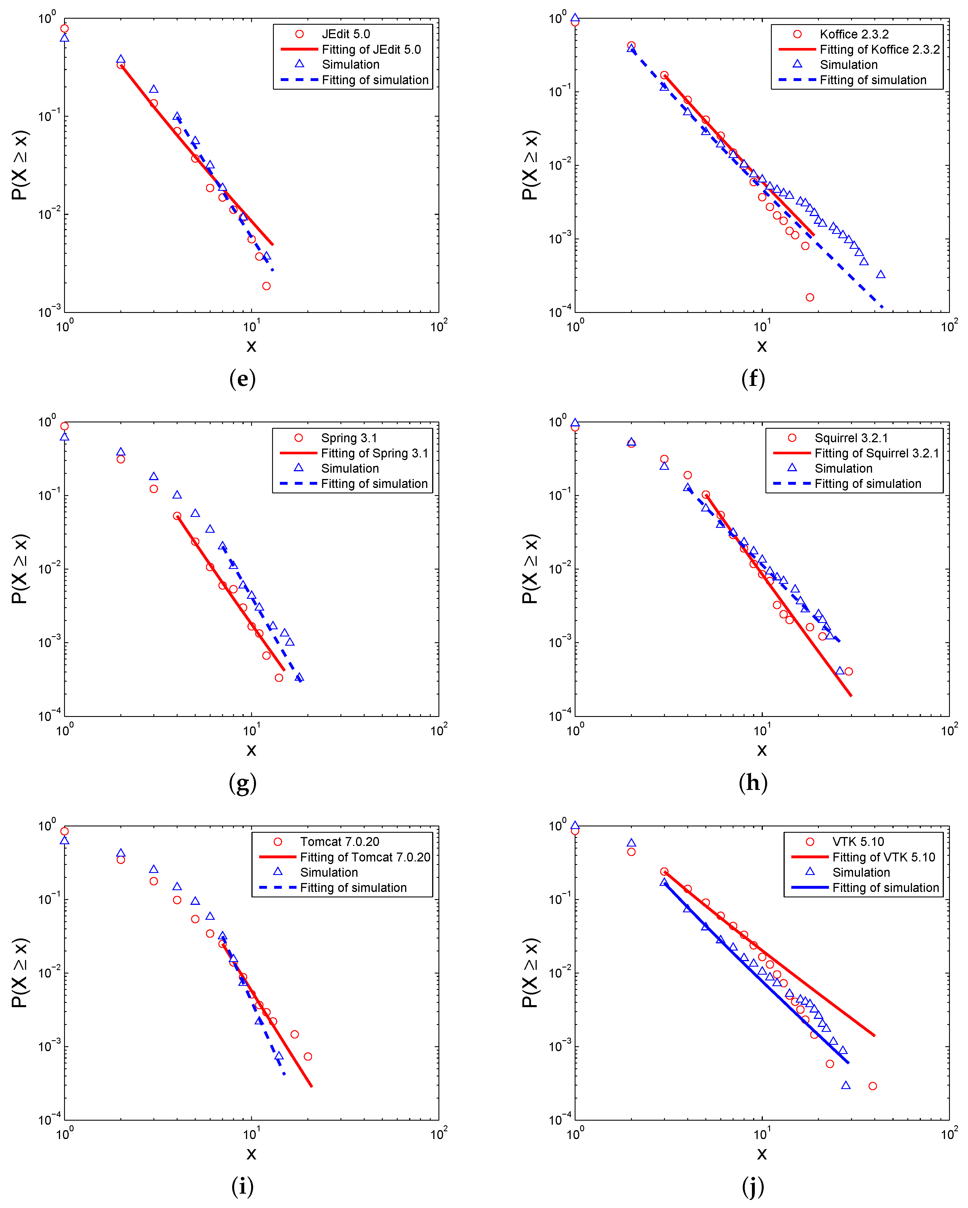
3.1. Degree Distributions

The degree of an element, $D_{i,j,k}$, is the number of edges attached to it. Correspondingly, the in-degree $D_{i,j,k}^{\mathrm{in}}$ and the out-degree $D_{i,j,k}^{\mathrm{out}}$ are respectively the number of links that enter it and the number of links that exit it.

In this study, the measurements of the p-value and $x_{\min }$ are used to measure the goodness-of-fit for degree distributions [50] (the code can be found from [51]). The first metric, p-value, represents the mathematical “distance” between the power-law distribution and the distribution of the actual network. The previous study reports that the power-law distribution of the current data can be believable, if p-value$\ge 0.1$; conversely, it cannot be authentic [50]. moreover, the degree distribution has some non-power-law behavior at the lower end; thus, we use the metric of $x_{\min }$ to control the part of the degree distribution that represents power-law behavior. It is reported that the power-law distribution is more plausible if the value of $x_{\min }$ is smaller [50].

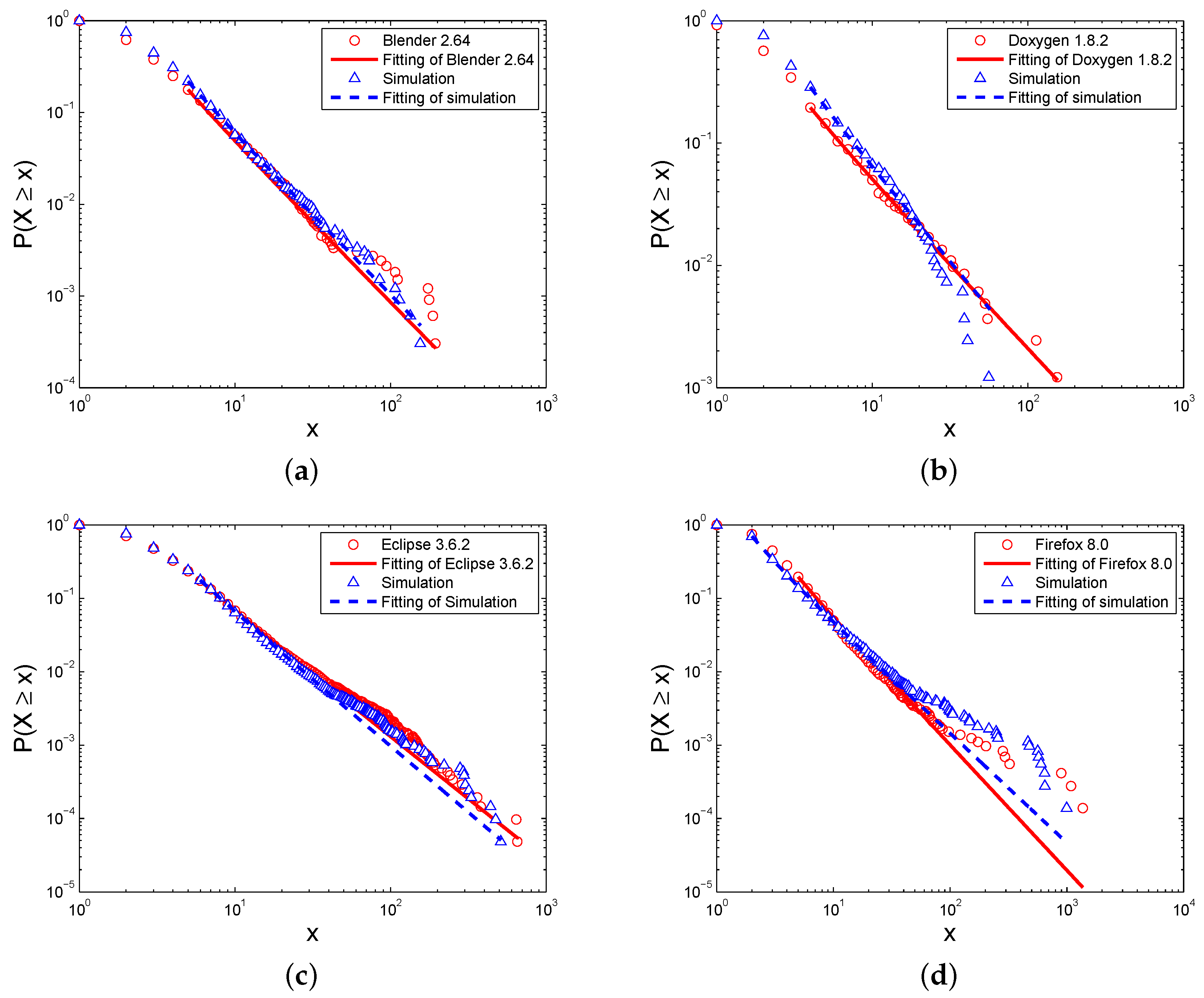
Figure 4 shows the simulated distribution of the degrees of the Level I elements, and the corresponding correlation coefficients, p-value, $x_{\min }$ can be found in

Table 2. Correlation coefficients of degree distributions; the corresponding metrics of the p-value and $x_{\min }$, produced by our multi-level model and real software systems.

Software	Real Networks			Simulations
	C-C	p-Value	$x_{\min }$	C-C	p-Value	$x_{\min }$
Blender 2.64	2.726	0.643	5	2.732	0.77	5
Doxygen 1.8.2	2.358	0.614	4	2.508	0.573	4
Eclipse 3.6.2	2.691	0.204	6	2.803	0.416	6
Firefox 8.0	2.705	0.14	5	2.488	0.196	2
Jedit 5.0	2.825	0.686	4	2.933	0.896	3
Koffice 2.3.2	2.657	0.332	3	2.825	0.51	4
Spring 3.1	2.923	0.605	5	2.731	0.378	2
Squirrel 3.2.1	2.719	0.24	4	2.801	0.432	5
Tomcat 7.0.20	2.605	0.152	4	2.89	0.582	3
VTK 5.10	2.513	0.655	8	2.348	0.259	3

. For comparison, in the same figure, we also plotted the degree distribution of the real software systems. It can be seen that both of and simulations and real software networks represent a power-law feature, and the degree distributions of the simulations are close to those of real software networks because the values of the exponents γ are close to the values of real software networks.

The power-law degree distribution is an important network feature in complex networks. It indicates that the degrees of most of the nodes are small while a small amount of nodes have large degrees [52]. In software networks, the elements with a small degree can be benefit fromthe function decomposition [53]. In contrast, the nodes with a large degree are crucial to achieve complex tasks and frequently interact and exchange data with other nodes. Therefore, the possible failures of these nodes with a large degree could greatly affect the system.

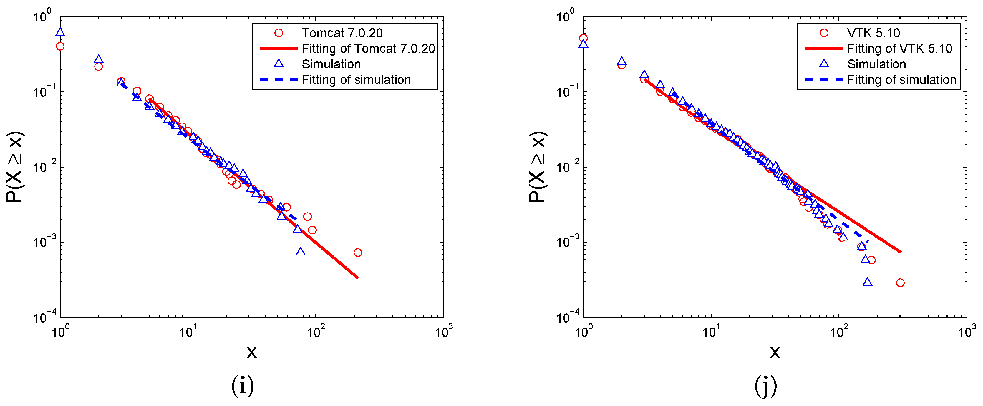
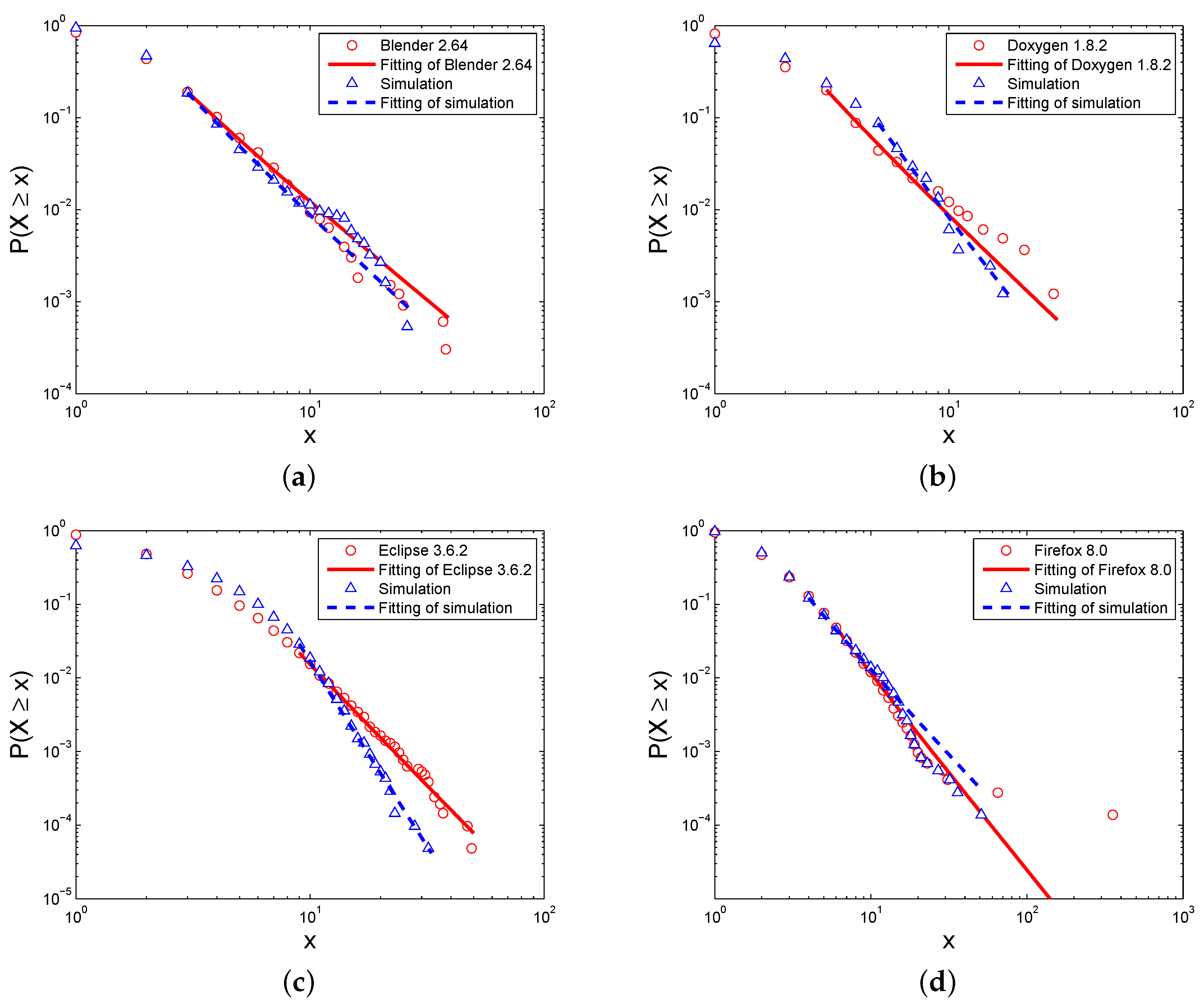
On the other hand, we know that software networks are directed; thus, the in-degree and out-degree distributions can also represent the interaction characteristics of the nodes. Figure 5 and

Table 3. Correlation coefficients of in-degree distributions; the corresponding metrics of the p-value and $x_{\min }$, produced by our multi-level model and real software systems.

Software	Real Networks			Simulations
	C-C	p-value	$x_{\min }$	C-C	p-value	$x_{\min }$
Blender 2.64	2.344	0.207	4	2.438	0.289	8
Doxygen 1.8.2	1.947	0.665	1	2.096	0.572	3
Eclipse 3.6.2	2.238	0.893	6	2.254	0.697	9
Firefox 8.0	2.262	0.609	3	2.105	0.196	4
Jedit 5.0	2.404	0.902	3	2.604	0.112	2
Koffice 2.3.2	2.322	0.08	4	2.293	0.744	5
Spring 3.1	2.478	0.605	4	2.349	0.724	6
Squirrel 3.2.1	2.072	0.176	3	1.992	0.161	3
Tomcat 7.0.20	2.426	0.902	5	2.257	0.537	3
VTK 5.10	2.106	0.145	3	2.258	0.126	5

show the simulated distribution of the in-degrees of the Level I elements, with the comparison of the in-degree distribution of the real software systems. Similar to the degree distributions, the in-degree distributions of the simulations and real software networks express the power-law, and the differences between them are small according to the exponents γ and fitting goodness p-value. Additionally, Figure 6 and

Table 4. Correlation coefficients of out-degree distributions; the corresponding metrics of the p-value and $x_{\min }$, produced by our multi-level model and real software systems.

Software	Real Networks			Simulations
	C-C	p-value	$x_{\min }$	C-C	p-value	$x_{\min }$
Blender 2.64	3.079	0.072	3	3.323	0.199	3
Doxygen 1.8.2	3.383	0.278	3	3.978	0.178	5
Eclipse 3.6.2	4.202	0.753	9	5.481	0.636	9
Firefox 8.0	3.762	0.625	6	3.534	0.144	4
Jedit 5.0	3.142	0.18	2	3.864	0.502	5
Koffice 2.3.2	3.536	0.06	3	3.442	0.14	4
Spring 3.1	4.443	0.387	4	5.223	0.665	7
Squirrel 3.2.1	4.373	0.843	5	3.438	0.275	4
Tomcat 7.0.20	4.915	0.795	7	6.038	0.605	7
VTK 5.10	3.078	0.05	3	3.491	0.16	3

show the out-degree distributions of these networks. Though the distributions are also close between the simulations and real software networks, the fitting goodness of the power-law is not good enough for some networks. Therefore, only some software networks follow a power-law.

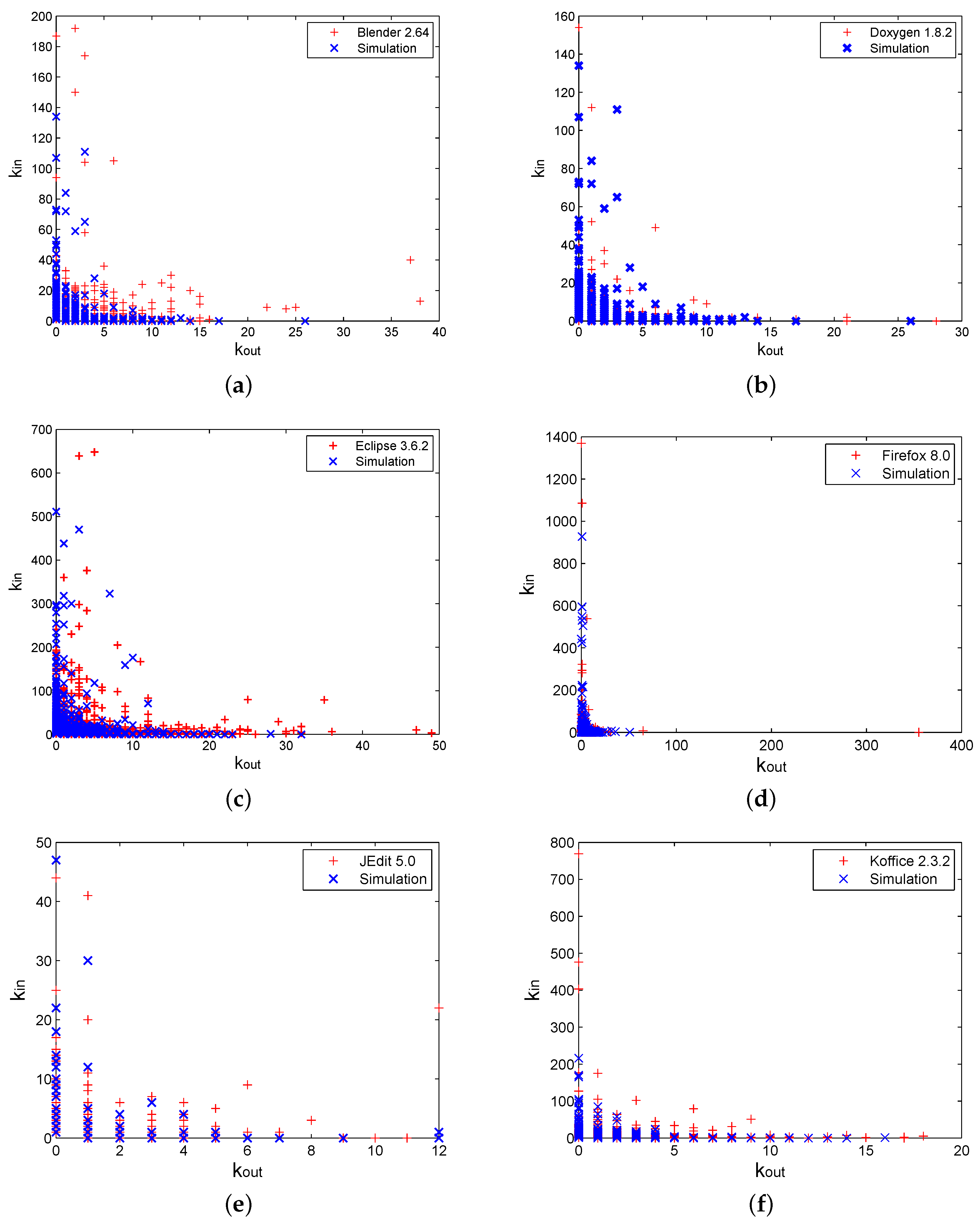
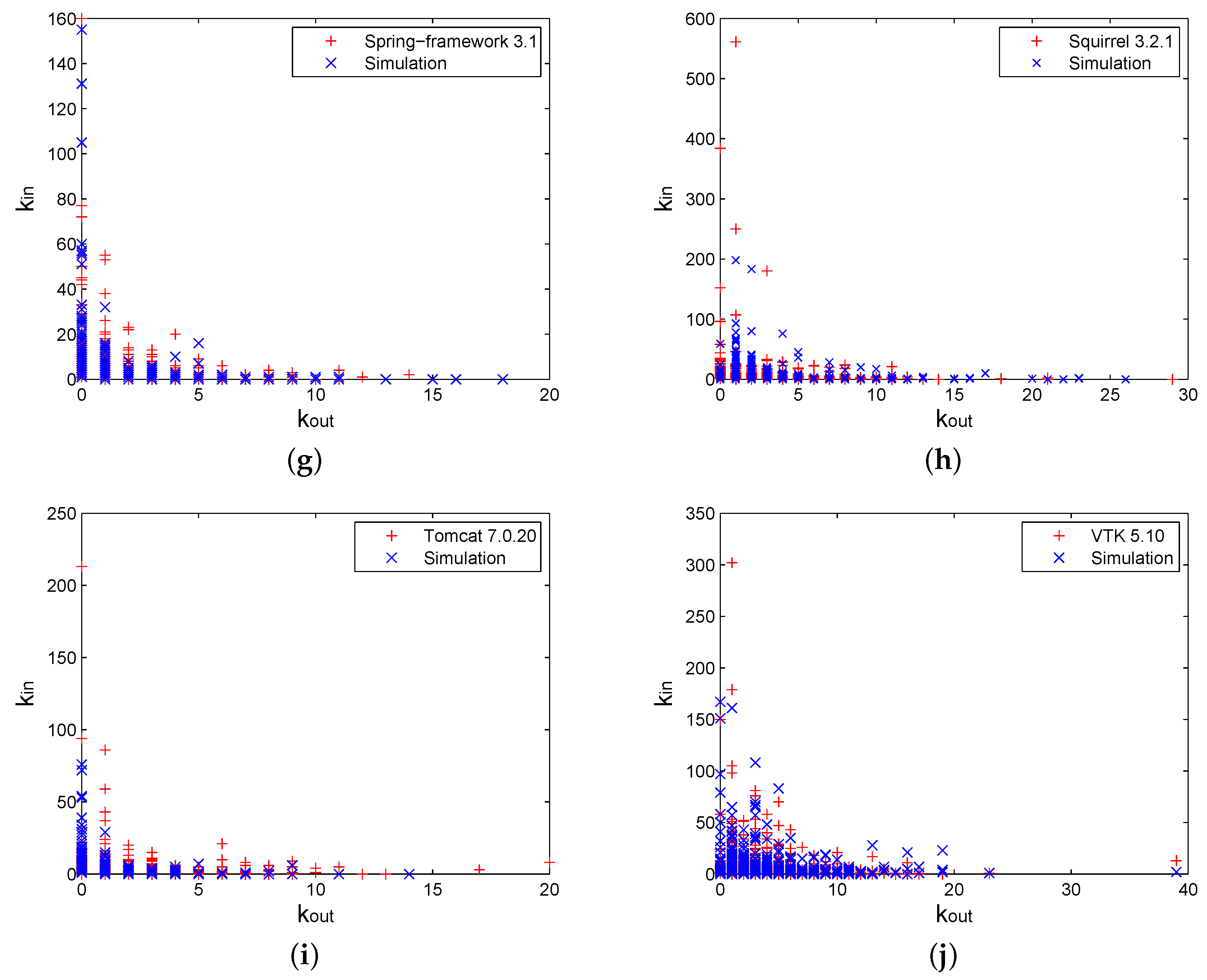
3.2. Correlation between In-Degree and Out-Degree

In comparison with some other complex networks, software networks display an important characteristic: in-degrees and out-degrees of elements are negatively correlated [11].

Figure 7 is a scatter plot of the simulated Level I in-degrees against corresponding out-degrees of all Level I elements. For comparison, in the same figure, we also plotted the same types of data obtained from the real software systems. This figure expresses that the results generated by our model are in line with empirical data.

We can see that the elements with larger in-degrees have smaller out-degrees, while the nodes with large out-degrees have smaller in-degrees. Therefore, we use correlation coefficient $R(D^{in},D^{out})$ for measuring the correlation between in-degree and out-degree distributions. The correlation coefficients of the in-degree set and the out-degree set (respectively for all nodes and the elements with $d^{\mathrm{in}}\ge 10$ or $d^{\mathrm{out}}\ge 10$) for simulations of the multi-level model and real software networks are shown in

Table 5. Correlation coefficients of the in-degree set and the out-degree set (respectively for all nodes and the elements with $d^{\mathrm{in}}\ge 10$ or $d^{\mathrm{out}}\ge 10$) for simulations of the multi-level model and real software networks. Sub-Network_1 and Sub-Network_2, respectively, represent the sub-network with the elements with $d^{\mathrm{in}}\ge 10$ or $d^{\mathrm{out}}\ge 10$ simulations of the multi-level model and the sub-network with the elements with $d^{\mathrm{in}}\ge 10$ or $d^{\mathrm{out}}\ge 10$ simulations of real software networks.

Software	Real Networks	Simulations (all d)	Sub-Network_1	Sub-Network_2
Blender 2.64	0.019	−0.116	−0.293	−0.536
Doxygen 1.8.2	−0.014	−0.029	−0.409	−0.43
Eclipse 3.6.2	−0.015	−0.09	−0.52	−0.494
Firefox 8.0	−0.025	−0.136	−0.448	−0.502
Jedit 5.0	0.042	−0.108	−0.372	−0.607
Koffice 2.3.2	−0.02	−0.071	−0.326	−0.461
Spring 3.1	−0.08	−0.133	−0.418	−0.482
Squirrel 3.2.1	−0.039	−0.056	−0.491	−0.525
Tomcat 7.0.20	−0.032	−0.08	−0.38	−0.449
VTK 5.10	−0.06	−0.127	−0.588	−0.511

. It can be seen that most of the coefficients for simulations ($-0.2\sim -0.05$) between in-degrees and out-degrees are close to the real software networks ($-0.2\sim 0$), though the negative correlations are not obvious. However, the correlation coefficients for simulations ($-0.4\sim -0.6$) between in-degrees and out-degrees are also close to the real software networks ($-0.3\sim -0.6$) and negatively correlated.

This negative correlation can be accounted for by some principles of software development. In a software system, elements with a large in-degree usually perform fundamental or commonly-used functions. These elements are therefore more likely to be reused. Conversely, elements with a large out-degree usually accomplish specific tasks. Therefore, they are less likely to be aggregated by other elements.

As shown in Figure 7, our model also reproduced another feature of real software systems, i.e., the largest out-degrees of the nodes are always much smaller than the largest in-degrees. In contrast, the BAmodel is unable to generate this attribute.

The reason for this feature is that elements that have a larger probability to be reused tend to have a higher in-degree; while existing elements are not easy to aggregate intonew elements. Additionally, a new element is more likely to reuse an element with many incoming links than a complex element with many outgoing links. The software engineering practice encourages reuse, which leads to large in-degrees. Conversely, it is not encouraged for an element to have too many out-degrees, because this will lead to highly complicated structures and hinder maintenance.

3.3. Level of Clustering and Modularity

In software design, the cohesion and coupling reflect the interactions between modules of software systems. Cohesion is a property of a single module and represents the degree to which the related units within the module, while coupling is a property of a pair of modules and represents the degree of relationships between such modules [41]. It is well known that the modularized software systems are much easier to develop and maintain, and a well-modularized software system usually represents a high degree of cohesion and a low degree of coupling [19,20].

According to the previous studies, the metrics of the clustering coefficient and modularity are used to represent the degree of cohesion and coupling for software networks [11,21]. The clustering coefficient of the entire network is a measure of the degree to which nodes in the network tend to cluster together, and it represents the tendency of the nodes’ neighbors to be their common neighbors in a network [11]. The modularity is an attribute of how good a network is divided into modules, and a good division is more edges within modules and fewer edges between them [54]. Comparatively speaking, the clustering coefficient tends to describe the clustering of the node and its neighbors, while the modularity emphasizes the goodness of module division.

The measurement of clustering coefficient C is the average of the clustering coefficients of all of the nodes [55]. The equation of the clustering coefficient is:

$$\begin{array}{c}\hfill C_{i,j,k}=\frac{t_{i,j,k}}{q_{i,j,k}(q_{i,j,k}-1)},\end{array}$$

in which $q_{i,j,k}$ is the number of nearest neighbors of node $v_{i,j,k}$ and $t_{i,j,k}$ is the number of connections between them. If the value of C is larger, the network tends to have a higher degree of cohesion and a lower degree of coupling.

Real software systems are modular, and the clusters represent some units that collaborate together to carry out the same task [56]. Then, we choose the sample software systems, such as Blender (written in C++) and Eclipse (written in Java), respectively, to generate 10 simulated networks for comparisons, and the results are shown in

Table 6. Clustering coefficients of Blender and Eclipse, with the corresponding simulations produced by the model for 8 versions.

Version Index	Blender	Simulations	Eclipse	Simulations
1	0.0574	$0.0642\pm 0.0027$	0.0565	$0.0629\pm 0.0032$
2	0.0545	$0.0651\pm 0.0034$	0.0572	$0.0633\pm 0.0027$
3	0.0568	$0.0676\pm 0.0025$	0.0616	$0.0639\pm 0.0039$
4	0.0642	$0.0684\pm 0.0047$	0.0605	$0.0642\pm 0.004$
5	0.0689	$0.0694\pm 0.0035$	0.0602	$0.0638\pm 0.0043$
6	0.0712	$0.0686\pm 0.005$	0.0599	$0.0655\pm 0.0029$
7	0.0757	$0.0699\pm 0.0053$	0.0582	$0.0663\pm 0.0036$
8	0.0651	$0.0705\pm 0.0045$	0.0601	$0.0669\pm 0.0041$

and

Table 7. The values of modularity of real software networks (Blender and Eclipse), with the corresponding simulations produced by the model for 8 versions.

Version Index	Blender	Simulations	Eclipse	Simulations
1	0.733	$0.787\pm 0.019$	0.719	$0.702\pm 0.024$
2	0.735	$0.799\pm 0.014$	0.722	$0.707\pm 0.033$
3	0.758	$0.813\pm 0.025$	0.716	$0.712\pm 0.018$
4	0.79	$0.818\pm 0.021$	0.714	$0.715\pm 0.03$
5	0.792	$0.821\pm 0.023$	0.727	$0.72\pm 0.024$
6	0.801	$0.827\pm 0.02$	0.72	$0.726\pm 0.031$
7	0.796	$0.832\pm 0.021$	0.726	$0.73\pm 0.024$
8	0.806	$0.835\pm 0.016$	0.732	$0.737\pm 0.028$

. Table 6 shows that the C value from our model is close to the value of the real-world software system. The reason is that the networks generated by the model are modular and have high cohesion.

The work in [21] proves that software networks show the feature of community structure by empirical studies, and thus, it is verified that software networks are modularized and that each consists of a network of interdependent parts [57]. Therefore, we use the metric of modularity Q, which is defined as the fraction of the edges within the divided groups minus the expected fraction of such edges in the network formed in a random way [54], to measure the modularity of software networks. The mathematical definition for modularity Q [58] is:

$$\begin{array}{c}\hfill Q=\frac{1}{2m}\sum _{i,j}[A_{ij}-\frac{k_i{k}_j}{2m}]\delta (c_i,c_j),\end{array}$$

where $A_{ij}$ denotes the weight of an edge between a node $v_i$ and a node $v_j$ (the weight is one in this case) in the graph, $k_i={\sum }_j{A}_{ij}$ is the sum of the weights of the edges attached to the node $v_i$, $c_i$ is the community to which the node $v_i$ is assigned, the function $\delta (u,v)$ is one if $u=v$ and zero otherwise and $m=\frac{1}{2}{\displaystyle \sum _{i,j}}{A}_{ij}$. The lager the value of Q, the higher the degree of cohesion for a network.

The examples of Blender and Eclipse are also used here to study the modularity of the simulations, and the results can be found in Table 7. We can see that the values of modularity are close between the real software networks and simulations. Moreover, the results also demonstrate that the model can produce software networks following the principle of high cohesion and low coupling.

4. Discussions

4.1. Trade-Off between Reusability and Maintainability

4.1.1. Cohesion and Coupling

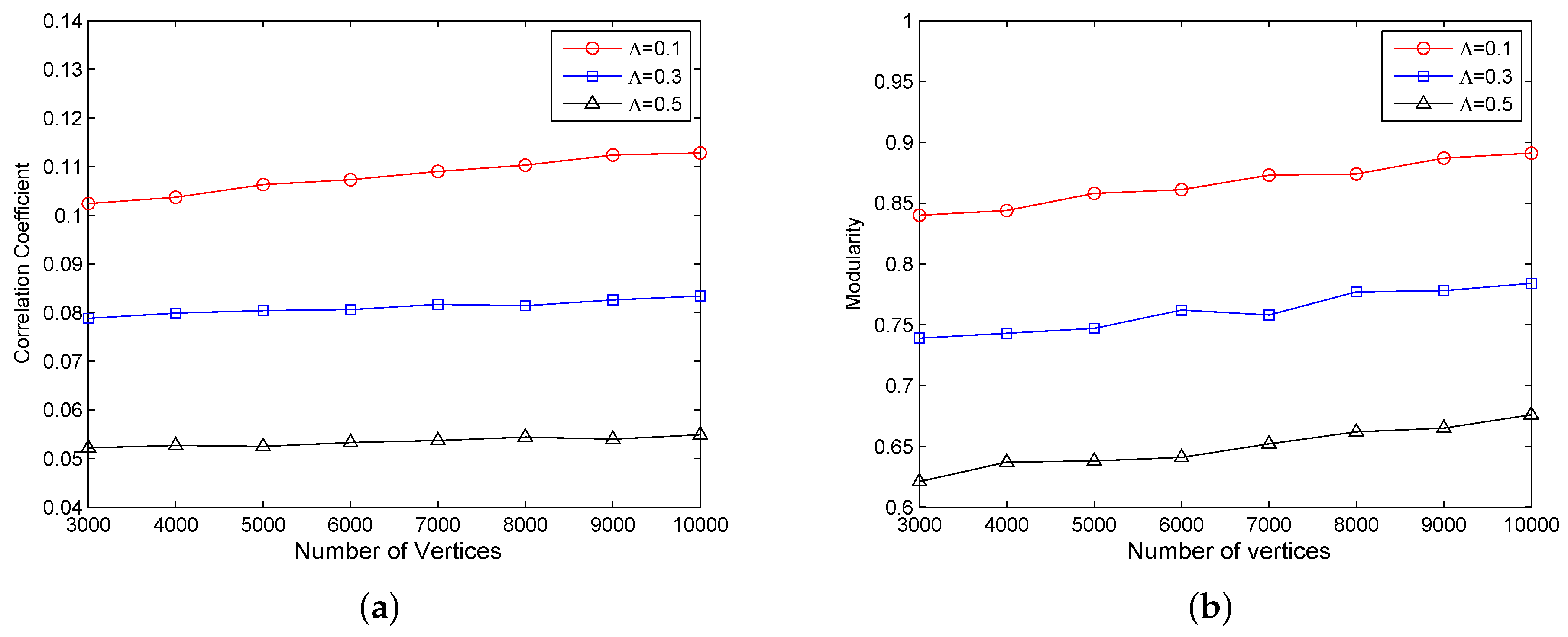
In the model, the coupling ratio Λ represents the possibility that a new edge connects two nodes in different modules, when new nodes are added to the existing network. Particularly, a larger value of Λ means a larger proportion of edges between nodes in different modules, which indicates that the nodes are more likely to connect the nodes in other modules. Conversely, a smaller value of Λ means a smaller proportion of edges between nodes in the same modules, which indicates that the nodes are more likely to connect the nodes in the same modules.

We generate three groups of evolving networks ($\mathsf{\Gamma }=0.8$, $N_{\mathrm{I},min}^{\mathrm{III}}=32$, $E_{\mathrm{I}}^{\mathrm{II}{,}^{\prime }}=48$ and $R_e=2$) by three different values of Λ, in order to discuss the clustering and modularity of the software networks for different coupling ratios. Figure 8 shows the negative correlation between the two measurements, clustering coefficient C and modularity Q, and coupling ratio Λ. We can see that the values of C distribute in the range of $0.1\sim 0.11$, and the values of Q are around $0.85$, when $\mathsf{\Lambda }=0.1$. However, the values of C decrease to the range of $0.05\sim 0.055$, and the values of Q decrease to around $0.65$ when the value of Λ rises to $0.5$. Therefore, the clustering coefficient and modularity will decrease as the coupling ratio becomes larger.

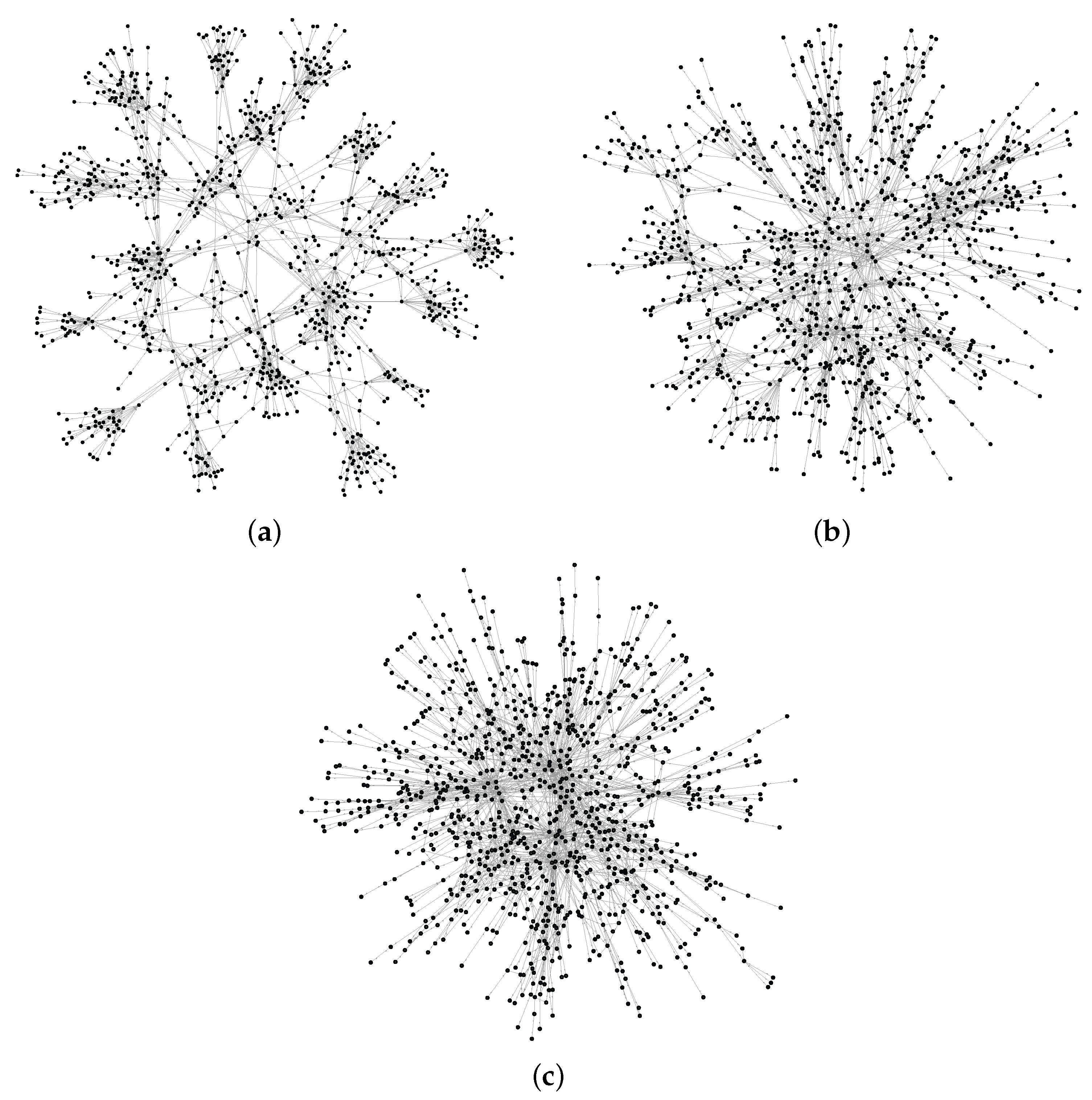
Moreover, the above correlation can be proven by the network topological structure. For the sake of better visualization, we generate three simulated networks ($\mathsf{\Gamma }=0.8$, $N_{\mathrm{I},min}^{\mathrm{III}}=32$, $E_{\mathrm{I}}^{\mathrm{II}{,}^{\prime }}=48$ and $R_e=2$) with 1000 nodes by different values of coupling ratio Λ and display the topological structure of them by Gephi (version 0.9) [59] in Figure 9. It can be seen clearly that the network represents obvious modularization as $\mathsf{\Lambda }=0.1$, and the nodes within the same modules connect more tightly while the connections between the nodes in different modules are sparse. As the value of Λ becomes $0.3$, the network still displays the feature of modularization, and the nodes interact with their neighbors within the modules more tightly than the nodes in other modules, although the modularization is reduced obviously. When the value of Λ reaches $0.5$, we cannot find a modular structure any longer from the generated network.

4.1.2. Reuse and Modularity

Software engineering practice encourages code reuse. However, reuse could lead to over coupling. In the case of a fixed amount of interactions across modules, if the value of Γ is large, more elements are reused as new elements are added. Conversely, if the value of Γ is small, existing modules aggregate more new elements.

Table 8. Numbers of Level I elements with large out-degrees, for different values of reuse probability Γ. The numbers 1 to 5 correspond respectively to the largest to the fifth largest out-degrees.

	1st	2nd	3rd	4th	5th
$\mathsf{\Gamma }=0.2$	192	186	142	137	133
$\mathsf{\Gamma }=0.4$	130	80	70	61	59
$\mathsf{\Gamma }=0.4$	126	47	34	32	31
$\mathsf{\Gamma }=0.8$	26	21	21	19	19

shows the top five largest out-degrees of the Level I network for different vales of reuse probability Γ and the corresponding numbers of the Level I elements. We can see that more elements with large out-degrees appear as the value Γ decreases. This will cause serious risk in global functions and decreases the evolvability of the software system, due to the complicated structure caused by many out-going edges.

Figure 9 also shows that the level of modularity is negatively related to coupling ratio Λ. In software engineering practice, the degree of modularity is governed by the trade-off between reuse and maintainability. In order to promote reuse, fine-grained and self-contained components should be used. If maintainability is a critical requirement, the coupling among components should be minimized by adopting relatively large-grain, highly cohesive components.

4.2. Influence of Motifs on Software Structure

In addition to modularity, software networks share another important feature with many other types of systems, such as biological networks. They show recurring patterns in a small scale, i.e., motifs. It has been conjectured that the abundance of motifs in software networks relates to universal mechanisms underlying software evolution [42].

From a specific angle based on our multi-level modeling, we have explored the impact of the existence of motifs on the structure of software systems. We undertake this exploration through the comparison between the simulated network with 10,000 nodes produced by our model in the normal setting ($\mathsf{\Lambda }=0.35$, $\mathsf{\Gamma }=0.8$, $N_{\mathrm{I},min}^{\mathrm{III}}=32$, $E_{\mathrm{I}}^{\mathrm{II}{,}^{\prime }}=64$ and $R_e=2$) and the resulting networks generated by special settings.

In the first special setting, all of the Level I elements within each Level II element are connected through the same mechanism as those Level II elements in each Level III element. The network generated by this rule also represents clustering, though the clustering coefficient C is smaller than the simulation with the motif, as shown in Figure 10. However, this formation rule does not conform to software engineering practices. Actually, the existing classes and components are usually reused, and this is the case of basic code reuse in software design. Besides, the local structures are also duplicated in some scenario, such as design patterns. If the latter is ignored in software design, it will result in an awful situation that some well-designed micro-structure (such as design patterns) will not be widely used, and the designers have to design many repeated scenarios and workflows. Thus, the motifs represent the micro-structure reuse in software system evolution.

In the second special setting, the random sub-graphs are used to replace the motifs. The result shows that the simulated network represents much stronger clustering than the simulation using motifs, as shown in Figure 10. The motifs used in software network formation are usually sparse sub-graphs, which are composed of three or four nodes and two or three edges. Conversely, the random sub-graphs include some dense sub-graphs, which will increase the clustering in the network formation. Most of the edges in these sub-graphs are redundant connections, and this could lead to unnecessary cost. Even worse, the McCabe cycles, which will result in increasing complexity and decreasing stability, will propagate in the evolution of the software systems. This discussion therefore tells us that the motifs can keep the overall software systems in reasonable cohesion and with structural stability.

5. Conclusions

The main contribution of this paper is that a multi-level model for software network evolution is proposed. In this model, three levels of elements, including class level, design pattern level and framework level, are used to describe the organization of the software systems. Through the comparisons with the real software networks from different aspects, the model has been proven to be inherently close to describing the formation process of real software systems. Furthermore, with the help of this model, we discuss some principles in software engineering practices, such as the relation of cohesion and coupling, the code reuse and modularity and the influence of motifs on software structure. This model could help us to understand the formation of the complex software systems and potentially to forecast the changes of the software structure.

However, some limitations may shorten the usage of the model. The parameters used in this model are obtained from the history data of the source codes. This means that the model may not correctly describe the structural changes due to the dramatic changes in the software architecture modifications. In addition, empirical studies tell us that the number of nodes and edges usually keeps increasing in most software projects, but it cannot avoid the sudden reduction of the nodes and edges in some projects for some unpredictable reasons. Besides, some large-scale software systems may not organize by three levels, but four levels or more, so how to dynamically describe the levels of the software network structure is also an open question.

Thus, some further studies still need to be done in the future. Firstly, more software projects should be investigated, especially the software systems written in the C language. Secondly, many projects have been terminated because of different reasons; thus, the studies of the structural changes of these software systems may make sense, then the model may be improved due to the further studies. Finally, the model may potentially be used to describe the formation of some other complex systems (such as the Internet, social networks, biology systems), and thus, it is worth updating the model to be universal for multi-level complex systems.

References

- Jeong, H.; Mason, S.; Barabási, A.-L.; Oltvai, Z.N. Lethality and centrality in protein networks. Nature 2001, 411, 41–42. [Google Scholar] [CrossRef] [PubMed]
- Newman, M.E.J. Scientific collaboration networks. I. Network construction and fundamental results. Phys. Rev. E 2001, 64, 016131. [Google Scholar] [CrossRef] [PubMed]
- Newman, M.E.J. Scientific collaboration networks. II. Shortest paths, weighted networks, and centrality. Phys. Rev. E 2001, 64, 016132. [Google Scholar] [CrossRef] [PubMed]
- Girvan, M.; Newman, M.E.J. Community structure in social and biological networks. Proc. Natl. Acad. Sci. USA 2002, 99, 7821–7826. [Google Scholar] [CrossRef] [PubMed]
- Ai, J.; Zhao, H.; Carley, K.M.; Su, Z.; Li, H. Evolution of IPv6 Internet topology with unusual sudden changes. Chin. Phys. B 2013, 22, 078902. [Google Scholar] [CrossRef]
- Wen, L.; Dromey, R.G.; Kirk, D. Software engineering and scale-free networks. IEEE Trans. Syst. Man Cybern. 2009, 39, 845–854. [Google Scholar]
- Concas, G.; Marchesi, M.; Pinna, S.; Serra, N. Power-laws in a large object-oriented software system. IEEE Trans. Softw. Eng. 2007, 33, 687–708. [Google Scholar] [CrossRef]
- Liu, J.; He, K.; Ma, Y.; Peng, R. Scale free in software metrics. In Proceedings of the 30th Annual International Computer Software and Applications Conference (COMPSAC ‘06), Chicago, IL, USA, 17–21 September 2006; pp. 229–235.
- Potanin, A.; Noble, J.; Frean, M.; Biddle, R. Scale-free geometry in OO programs. Commun. ACM 2005, 48, 99–103. [Google Scholar] [CrossRef]
- Ma, Y.; He, K.; Du, D.; Liu, J.; Yan, Y. A complexity metrics set for large-scale object-oriented software systems. In Proceedings of the 6th IEEE International Conference on Computer and Information Technology (CIT ‘06), Seoul, Korea, 20–22 September 2006; pp. 189–194.
- Myers, C.R. Software systems as complex networks: Structure, function, and evolvability of software collaboration graphs. Phys. Rev. E 2003, 68, 046116. [Google Scholar] [CrossRef] [PubMed]
- Valverde, S.; Sol, R.V. Hierarchical small worlds in software architecture. Dyn. Contin. Discret. Impuls. Syst. Ser. B 2007, 14, 1–11. [Google Scholar]
- Li, B.; Pan, W.; Lu, J. Multi-granularity dynamic analysis of complex software networks. In Proceedings of the 2011 IEEE International Symposium on Circuits and Systems (ISCAS), Rio de Janeiro, Brazil, 15–18 May 2011; pp. 2119–2124.
- Jenkins, S.; Kirk, S.R. Software architecture graphs as complex networks: A novel partitioning scheme to measure stability and evolution. Inf. Sci. 2007, 177, 2587–2601. [Google Scholar] [CrossRef]
- Canfora, G.; Cerulo, L.; Cimitile, M.; Penta, M.D. How changes affect software entropy: An empirical study. Empir. Softw. Eng. 2014, 19, 1–38. [Google Scholar] [CrossRef]
- Pan, W.; Li, B.; Ma, Y.; Qin, Y.; Zhou, X. Measuring structural quality of object-oriented softwares via bug propagation analysis on weighted software networks. J. Comput. Sci. Technol. 2010, 25, 1202–1213. [Google Scholar] [CrossRef]
- Zhang, H.; Zhao, H.; Cai, W.; Zhao, M.; Luo, G. Visualization and cognition of large-scale software structure using the k-core analysis. In Proceedings of the 2008 International Conference on Intelligent Information Hiding and Multimedia Signal Processing, Harbin, China, 15–17 August 2008; pp. 954–957.
- Dabrowski, R.; Stencel, K.; Timoszuk, G. Software is a directed multigraph. In Software Architecture; Springer: Berlin/Heidelberg, Germany, 2011; pp. 360–369. [Google Scholar]
- Zanetti, M.S.; Schweitzer, F. A network perspective on software modularity. In Proceedings of the 25th International Conference on Architecture of Computing Systems (ARCS) Workshops, München, Germany, 28–29 February 2012; pp. 1–8.
- Praditwong, K.; Harman, M.; Yao, X. Software module clustering as a multi-objective search problem. IEEE Trans. Softw. Eng. 2011, 37, 264–282. [Google Scholar] [CrossRef]
- Šubelj, L.; Bajec, M. Community structure of complex software systems: Analysis and applications. Physica A 2011, 390, 2968–2975. [Google Scholar] [CrossRef]
- Meyer, P.; Siy, H.; Bhowmick, S. Identifying important classes of large software systems through k-core decomposition. Adv. Complex Syst. 2014, 17, 1550004. [Google Scholar] [CrossRef]
- Zanetti, M.S.; Scholtes, I.; Tessone, C.J.; Schweitzer, F. Categorizing Bugs with Social Networks: A Case Study on Four Open Source Software Communities. In Proceedings of the 2013 International Conference on Software Engineering, San Francisco, CA, USA, 2013; pp. 1032–1041.
- Zhang, W.; Nie, L.; Jiang, H.; Chen, Z.; Liu, J. Developer Social Networks in Software Engineering: Construction, Analysis, and Applications. Sci. China Inf. Sci. 2014, 57, 1–23. [Google Scholar] [CrossRef]
- Xuan, Q.; Fu, C.; Yu, L. Ranking developer candidates by social links. Adv. Complex Syst. 2014, 17, 1550005. [Google Scholar] [CrossRef]
- Li, P.; Zhao, H.; Li, H.; Liu, Z. Research of Software Network Measurement Based on The Deviation of Standard Entropy. J. Northeast. Univ. 2010, 31, 1558–1561. (In Chinese) [Google Scholar]
- Miranskyy, A.V.; Davison, M.; Reesor, R.M.; Murtaza, S.S. Using entropy measures for comparison of software traces. Inf. Sci. 2012, 203, 59–72. [Google Scholar] [CrossRef]
- Safar, M.H.; Sorkhoh, I.Y.; Farahat, H.M.; Mahdi, K.A. On Maximizing the Entropy of Complex Networks. Procedia Comput. Sci. 2011, 5, 480–488. [Google Scholar] [CrossRef]
- Wang, L.; Wang, Z.; Yang, C.; Zhang, L. Evolution and stability of Linux kernels based on complex networks. Sci. China Inf. Sci. 2012, 54, 1972–1982. [Google Scholar] [CrossRef]
- Turnu, I.; Concas, G.; Marchesi, M.; Tonelli, R. The fractal dimension of software networks as a global quality metric. Inf. Sci. 2013, 245, 290–303. [Google Scholar] [CrossRef]
- Cataldo, M.; Scholtes, I.; Valetto, G. A complex networks perspective on collaborative software engineering. Adv. Complex Syst. 2014, 17, 1430001. [Google Scholar] [CrossRef]
- Wang, L.; Wang, P. Propagation and stability in software: A complex network perspective. Int. J. Mod. Phys. C 2015, 26, 1550052. [Google Scholar] [CrossRef]
- Koch, S. Software evolution in open source projects—A large-scale investigation. J. Softw. Maint. Evol. Res. Pract. 2007, 19, 361–382. [Google Scholar] [CrossRef]
- Cai, K.; Yin, B. Software execution processes as an evolving complex network. Inf. Sci. 2009, 179, 1903–1928. [Google Scholar] [CrossRef]
- Israeli, A.; Feitelson, D.G. The Linux kernel as a case study in software evolution. J. Syst. Softw. 2010, 83, 485–501. [Google Scholar] [CrossRef]
- Zheng, X.; Zeng, D.; Li, H.; Wang, F. Analyzing open-source software systems as complex networks. Physica A 2008, 387, 6190–6200. [Google Scholar] [CrossRef]
- Pan, W.; Li, B.; Ma, Y.; Liu, J. A Novel Software evolution model based on software networks. In Complex Sciences; Springer: Berlin/Heidelberg, Germany, 2009; pp. 1281–1291. [Google Scholar]
- He, K.; Peng, R.; Liu, J.; He, F.; Lian, P.; Li, B. Design methodology of networked software evolution growth based on software patterns. J. Syst. Sci. Complex 2006, 19, 157–181. [Google Scholar] [CrossRef]
- Theodore, C.; Alexander, C. Forecasting Java Software Evolution Trends Employing Network Models. IEEE Trans. Softw. Eng. 2015, 41, 582–602. [Google Scholar]
- LaBelle, N.; Wallingford, E. Inter-Package Dependency Networks in Open-Source Software. 2004; arXiv:0411096v1. [Google Scholar]
- Stevens, W.P.; Myers, G.J.; Constantine, L.L. Structured design. IBM Syst. J. 1974, 13, 115–139. [Google Scholar] [CrossRef]
- Valverde, S.; Solé, R.V. Network motifs in computational graphs: A case study in software architecture. Phys. Rev. E 2005, 72, 026107. [Google Scholar] [CrossRef] [PubMed]
- Ma, Y.; He, K.; Liu, J. Network motifs in object-oriented software systems. 2008; arXiv:0808.3292. [Google Scholar]
- Pan, W.; Li, B.; Ma, Y.; Liu, J. Multi-granularity evolution analysis of software using complex network theory. J. Syst. Sci. Complex 2011, 24, 1068–1082. [Google Scholar] [CrossRef]
- Li, H.; Hao, L.; Chen, R.; Ge, X.; Zhao, H. Symmetric Preferential Attachment for New Vertices Attaching to Software Networks. New Gener. Comput. 2014, 32, 271–296. [Google Scholar] [CrossRef]
- Gu, Q.; Chen, D. Validation and simulation of software system evolution rules using software networks. Sci. Sin. Inf. 2014, 44, 20–36. [Google Scholar]
- Stevens, W.P.; Myers, G.J.; Constantnve, L.L. Structured design. IBM Syst. J. 1999, 38, 231–256. [Google Scholar] [CrossRef]
- Schweitzer, F.; Nanumyan, V.; Tessone, C.J.; Xia, X. How do OSS projects change in number and size? A large-scale analysis to test a model of project grwoth. Adv. Complex Syst. 2014, 17, 1550008. [Google Scholar] [CrossRef]
- Tessone, C.J.; Geipel, M.M.; Schweitzer, F. Sustainable growth in complex networks. Europhys. Lett. 2011, 96, 58005. [Google Scholar] [CrossRef]
- Clauset, A.; Shalizi, C.R.; Newman, M.E.J. Power-Law Distributions in Empirical Data. SIAM Rev. 2009, 51, 661–703. [Google Scholar] [CrossRef]
- Fitting power-law distributions to empirical data. Available online: https://github.com/ntamas/plfit (accessed on 6 May 2016).
- Barabási, A.-L.; Albert, R. Emergence of scaling in random networks. Science 1999, 286, 509–512. [Google Scholar] [PubMed]
- Gao, J.; Wang, J.; Yin, M. Experimental analyses on phase transitions in compiling satisfiability problems. Sci. China Inf. Sci. 2015, 58, 032104. [Google Scholar] [CrossRef]
- Newman, M.E.J.; Girvan, M. Finding and evaluating community structure in networks. Phys. Rev. E 2004, 69, 026113. [Google Scholar] [CrossRef] [PubMed]
- Watts, D.J.; Strogatz, S.H. Collective dynamics of ‘small-world’ networks. Nature 1998, 393, 440–442. [Google Scholar] [CrossRef] [PubMed]
- Fortuna, M.A.; Bonachela, J.A.; Levin, S.A. Evolution of a Modular Software Network. Proc. Natl. Acad. Sci. USA 2011, 108, 19985–19989. [Google Scholar] [CrossRef] [PubMed]
- Subelj, L.; Zitnik, S.; Blagus, N.; Bajec, M. Node mixing and group structure of complex software networks. Adv. Complex Syst. 2014, 17, 1450022. [Google Scholar] [CrossRef]
- Blondel, V.D.; Guillaume, J.-L.; Lambiotte, R.; Lefebvre, E. Fast unfolding of communities in large networks. J. Stat. Mech. Theory Exp. 2008, 2008, P10008. [Google Scholar] [CrossRef]
- The Open Graph Viz Platform. Available online: https://gephi.github.io/ (accessed on 6 May 2016).
Figure 1.
An example of the extraction from a software system to a software network. (a) The Unified Modeling Language (UML) graph of the simple software program; (b) the software network extracted by the software program on the left.
Figure 2.
Most commonly-used motifs in software networks. (a–d) are 3-node motifs; (e–n) are 4-node motifs. All of the motifs are sparse graphs and not directed cycle.
Figure 3.
Structure and evolutionary mechanism of a multi-level software system.
Figure 4.
Degree distributions produced by our multi-level model (○ points) (the scale of the vertical axis is logarithmic). The corresponding distributions of real software systems (△ points) are also plotted here for comparison. (a) Blender 2.64; (b) Doxygen 1.8.2; (c) Eclipse 3.6.2; (d) Firefox 8.0; (e) JEdit 5.0; (f) Koffice 2.3.2; (g) Spring 3.1; (h) Squirrel 3.2.1; (i) Tomcat 7.0.20; (j) VTK 5.10.
Figure 5.
In-degree distributions produced by our multi-level model (○ points) (the scale of the vertical axis is logarithmic). The corresponding distributions of real software systems (△ points) are also plotted here for comparison. (a) Blender 2.64; (b) Doxygen 1.8.2; (c) Eclipse 3.6.2; (d) Firefox 8.0; (e) JEdit 5.0; (f) Koffice 2.3.2; (g) Spring 3.1; (h) Squirrel 3.2.1; (i) Tomcat 7.0.20; (j) VTK 5.10.
Figure 6.
Out-degree distributions produced by our multi-level model (○ points) (the scale of the vertical axis is logarithmic). The corresponding distributions of real software systems (△ points) are also plotted here for comparison. (a) Blender 2.64; (b) Doxygen 1.8.2; (c) Eclipse 3.6.2; (d) Firefox 8.0; (e) JEdit 5.0; (f) Koffice 2.3.2; (g) Spring 3.1; (h) Squirrel 3.2.1; (i) Tomcat 7.0.20; (j) VTK 5.10.
Figure 7.
Simulated in-degrees against corresponding out-degrees. The corresponding data obtained from the real software networks (+ points) and those of simulations (× points) are also plotted here for comparison. (a) Blender 2.64; (b) Doxygen 1.8.2; (c) Eclipse 3.6.2; (d) Firefox 8.0; (e) JEdit 5.0; (f) Koffice 2.3.2; (g) Spring 3.1; (h) Squirrel 3.2.1; (i) Tomcat 7.0.20; (j) VTK 5.10.
Figure 8.
Negative correlation between two measurements and coupling ratio Λ. (a) The correlation between clustering coefficient C and coupling ratio Λ; (b) The correlation between modularity Q and coupling ratio Λ.
Figure 9.
The structure of the Level I network for different values of coupling ratio Λ. (a) ; (b) ; (c) .
Figure 10.
The influence of motifs on the values of the clustering of Level I networks.