Information and Selforganization: A Unifying Approach and Applications

Abstract

Selforganization is a process by which the interaction between the parts of a complex system gives rise to the spontaneous emergence of patterns, structures or functions. In this interaction the system elements exchange matter, energy and information. We focus our attention on the relations between selforganization and information in general and the way they are linked to cognitive processes in particular. We do so from the analytical and mathematical perspective of the “second foundation of synergetics” and its “synergetic computer” and with reference to several forms of information: Shannon’s information that deals with the quantity of a message irrespective of its meaning, semantic and pragmatic forms of information that deal with the meaning conveyed by messages and information adaptation that refers to the interplay between Shannon’s information and semantic or pragmatic information. We first elucidate the relations between selforganization and information theoretically and mathematically and then by means of specific case studies.

1. Introduction

1.1. Goal

In this paper we want to elucidate the relation between self-organization and information. By the term information we refer to Shannon information (SHI), pragmatic information (PI), semantic information (SI) and the relations between these three information forms that we recently [1] described as information adaptation (IA). We intend to search for universal principles in the inanimate and animate (conscious) world—an intention, which is in line with previous approaches by Norbert Wiener’s cybernetics [2], Heinz von Foerster’s cybernetics of the second order [3], Ludwig von Bertalanffy’s general systems theory [4] and Synergetics—Hermann Haken’s theory of Selforganization [5,6,7]. In what follows we elaborate on Synergetics’ treatment of information theory and self-organization in a way that may help understand neuronal self-organization and its perceptual correlates. We start with a didactic introduction to the basic notions of self-organization and information theory, developing some of the deeper principles of synergetics in a heuristic way. We then develop the mathematical formalisms that substantiate the ideas to highlight emergent properties that may have special relevance for understanding perceptual synthesis in the brain. The paper concludes by looking at the remarkable consilience between the formal results and the dynamics implicit in neuronal responses and perception; for example, bi-stable perception and the way that we deploy saccadic eye movements to sample our sensorium.

1.2. Conceptualization

1.2.1. Selforganization

Selforganization (SO) is a property of open and complex systems, composed of parts, elements, components and units, whose network of interactions serves for the exchange of matter, energy and information among their parts and with their surroundings (cf. Figure 1). A case in point is the flower in Figure 2 that, as a complex system, interacts with its surrounding environment by exchanging light, water, minerals, O₂ and CO₂. This exchange is rather unspecific, i.e., it does not act like a “sculptor” who shapes, say a statue; rather such a system organizes its structure and function spontaneously by itself; hence the notion of selforganization.

Another important property of such systems is emergence: By means of self-organization new properties that do not exist in the parts emerge with the implication that “the whole is greater than the sum of its parts”—a statement attributed to Aristotle [8]. This is also the basic meaning of the notion “Synergy” the definition of which in Wikipedia (April 2015) starts with the sentence: “Synergy is the creation of a whole that is greater than the simple sum of its parts”.

While the notion of selforganization has been ventilated in philosophy since antiquity [9], it was introduced into science by Ashby [10] in 1947. Ashby treats the nervous system, particularly the cerebral cortex, as purely physical dynamical system. He shows that such a system makes a transition from one “equilibrium state” to a different one, when an otherwise constant parameter is changed. As it will transpire below, his paper is quite of relevance to our article. Prigogine [11] conceived pattern formation of physical and chemical systems under nonequilibrium conditions, (cf. Figure 3 below) as processes of selforganization and developed, in the realm of thermodynamics the “excess entropy production principle”. Nicolis, in the past Prigogine’s student, carried the field further by applying kinetic equations to chemical reaction models (the “Brusselator”) [11]. For further details of Nicolis’ work see his contribution to this special issue. Haken’s contribution to the theory of selforganization cf. [12,13], inspired as it is by his laser theory [14], is outlined below.

In particular Synergetics [7,12,13] has developed universal principles that apply to both the inanimate and animate (conscious) worlds. The link between the two worlds was made by analogy between pattern formation in the inanimate domain and pattern recognition in the animate domain. A case in point is the Bénard [15] convection of a liquid in a circular vessel heated from below and cooled from above (Figure 3): At a small temperature difference between the bottom and the top of the liquid $\Delta =T_2-T_1$ heat is transported by conduction (Figure 3a) where no macroscopic structure appears. If ∆ exceeds a critical value, a macroscopic pattern in the form of up-and down-welling (convection) rolls appears (Figure 3b), whereas in a circular vessel hexagonal cells appear (Figure 3c cf. for instance [7]).

According to Synergetics, the temperature difference of our example (Figure 3) acts as control parameter. If $T_2-T_1>{\Delta }_{\text{critical}}$, that is, if the control parameter (i.e., temperature difference) crosses a critical threshold, we observe instability out of which a new structure appears. As is shown by a detailed mathematical approach in Synergetics [7], close to such instability points new collective variables appear; they are called order parameters (OPs) and once they emerge, they “enslave” all the elements and parts of the system to their specific dynamics. The OPs thus emerge bottom-up out of the interaction between the parts of the system, however, once they emerge, the system is being top-down governed by one or a few order parameters (as illustrated in Figure 4). We call this mutual relationship between bottom-up and top-down causation “circular causality”. For example, in the case of Figure 3b, the OP parameter determines the movement of the many parts (molecules) of which the system “liquid” is composed. In the parlance of Synergetics this phenomenon is called the slaving principle. In mathematical terms (cf. also below): If the OPs are denoted by ${\xi }_j(t),j=1,\dots ,M$, t: time, and the variables of the elements, by $q_l(t),l=1,\dots ,N$, then $q_l(t)=f_l({\xi }_1,\dots ,{\xi }_M)$. The crucial insight is that M << N.

This process implies an enormous complexity reduction concerning information channels. While in the original network with N parts and long-range interactions there are up to (about) $N^2$ information channels (N parts exchange information with the other $N-1$ parts, i.e., $N\left(N-1\right)\approx N^2$ channels altogether). Now we have to deal with 2NM channels among order parameters and parts and M² channels among OPs, i.e., 2NM + M² << N² channels altogether. Thus the high dimensional dynamics is reduced to a low-dimensional dynamics.

The synergetic approach to mind/brain pattern recognition is analogous to the above process of pattern formation in matter (Figure 5): Now the parts are the features of a pattern. These features, e.g., the grey values of the pixels of an image (“pattern”), are projected through the visual system of a human to feature-specific neurons that interact by the exchange of information leading to the formation of OPs that compete with other OPs (governing other feature-configurations). Eventually, the OP with the strongest support will win and will force the system to exhibit the complete set of features belonging to that OP. The offered (incomplete) pattern is recognized. The result is full correspondence between the complementation process during pattern formation and the associative memory during pattern recognition. What we just described can be, and has been, cast into an algorithm that defines the synergetic computers (SC).

1.2.2. Information

Information as employed here is a basic property and process of open and complex systems—a means by which the system and its parts extract, or produce meaning and/or action from signals. These processes of information production, extraction and exchange evolve spontaneously, i.e., by selforganization.

Shannon Information

A seminal step in the study of information was Shannon’s [16] “Mathematical theory of communication” which demonstrated that information could be quantified regardless of the specific meaning the signals/message convey; we refer to it below as Shannon’s or Shannonian information (SHI) (cf. Equation (1) below). Shannon Information theory has since become central to the development of computer technology and science, communication and information sciences, cognitive sciences, to name but a few of the more dominant domains.

Forms of Information

The publication of Shannon’s seminal paper was followed by attempts at formal definitions of information with meaning, that is, SI that refers to meaning per-se (for reviews see [17,18]), and PI that refers to action (see review in [19]). In our recent monograph [6] we show, firstly, that SHI and SI interact as two aspects of a process of information adaptation (IA) in which SHI triggers SI, while the later participates in the determination of SHI. Secondly, that in cognition, IA is implemented by means of information inflation or deflation the function of which is to adapt the quantity of information entering the mind/brain/body (MBB) to its information processes capabilities and to the SI/PI generated by the MBB. Our empirical basis was Hubel and Wiesel seminal findings [20,21,22] and subsequent studies [23,24,25], who showed that visual perception evolves as follows (Figure 6): data from the world is first analyzed (“deconstructed” in Kandel’s [25] words) by the mind/brain, in a bottom-up manner, into local information of lines, corners, etc. This local information triggers a top-down process of synthesis (“reconstruction” in Kandel’s [25] language) that gives rise to global information, that is, to seeing and recognition. (For more details see [6]).

Another example [6] of IA that nicely illustrates the dynamic interplay between SHI, SI and IA, is the approaching lady scenario (Figure 7): Imagine you stand in an open area (say, on the sea shore) and you observe at the horizon an object moving towards you. At this stage there is little data and the object can be anything and thus the SHI (uncertainty) is high. As the object gets closer, more data are added and you realize that it is a person, that is, your MBB adapts to the incoming data by deflating the SHI (uncertainty) and by pattern recognizing the moving object as a the SI category “person”. As this person gets still closer …, you realize that it is the SI category “woman”—… Finally, as this woman gets even closer you realize that this is Eve—…

1.2.3. Information and Embodied Cognition

An interesting implication of IA is that both SI and PI refer to bodily action: PI to externally observed action which is commonly termed behavior, while SI to internally observed action such as perception, which due to technological advance can be observed (at least partially) by fMRI, EEG and the like. Such links between action, SI and PI, shed new light on notions associated with embodied cognition (EC). EC [27] is often interpreted in terms of complexity, suggesting that organisms’ body, mind and environment form a complex, adaptive, interactive system. In this interaction, the system’s elements exchange matter, energy and information. However, what does it mean that the system’s elements exchange information? We answer this question by reference to three forms of information—SHI, SI or PI, and the process of IA introduced above.

First answer: the system’s elements exchange SHI. Applied to EC we define SHI as a measure of the number of actions an object or environment affords to a specific organism with specific body and mental properties. (As we show in some details in Appendix F below, there is a close relation with the concept of “empowerment” of Klyubin et al [28]). Consider the example of a frog. According to Maturana et al. [29], its reflective action is determined by specific cues: Small, fast moving object implies prey and the action attack (Figure 8a); while large, slowly moving object implies predator and the action flight. Since in both cases the frog has no choice, its SHI = 0. We term this as reflexive action. On the other hand, the cat in Figure 8b has a choice between two optional actions: flight or climb. Its SHI is, thus 1 bit of information. Here we are dealing with perceptive action—the “classical” case of EC.

Second answer: the system’s elements exchange meaning in the form of SI or PI. Following Haken [1], we define information with meaning (SI or PI) as a message that has specific effect on a receiver, when the receiver is modeled as a dynamical system that has a number of attractor states. The messages (signals) carrying meaning are considered different if they cause the dynamical system to reach different attractor states (see also [30,31]). These attractor states might be SI attractors as in Figure 9, where the figure at the center might be a bull, mountain goat, buffalo or a gnou; or PI as in Figure 8b, where the cat has a choice between two actions.

Third answer: the system’s elements perform an interplay between SHI and SI/PI. As noted above, IA refers to a process in which SHI generates SI/PI, while the latter control SHI. The above examples of vision (Figure 6) and the approaching lady (Figure 7) nicely illustrate the play between SHI and SI (for further discussion cf. Section 4.2 below). A third example, specifically related to PI, is the finger movement experiment and paradigm [32].

A typical such experiment starts with the following PI behavioral task (Figure 10): A test person is asked to move his/her index fingers in parallel at the speed of the metronome, which begins in a low speed. Then with increasing speed of the metronome, at a critical value, the finger movements of the test person undergo involuntarily a switch to a symmetric coordination. Note that if on the initial stage the test-person is not instructed to move the index fingers in parallel, he or she has a choice between two options, that is, between the two stable states (parallel/symmetric) allowing voluntary behavior. In such a situation the person has the freedom to choose between states 1 and 2 of a single OP (the relative phase between the index fingers). Here the PI determined Shannon information i = 1. This form of behavior applies up to a certain threshold of finger movement speed. Once this threshold is crossed, there is an involuntary transition behavior in which only one specific OP value that can be realized and dominates the system. Here, the PI determined Shannon information i = 0. This description is a rough approximation, however; a refined mathematical approximation is developed below in Section 9, together with additional examples.

1.3. The Second Foundation of Synergetics

Since in the case of humans the various forms of information are brought about by the human mind/brain, some relevant aspects must be considered here. Starting from the notion that the (human) brain is a highly complex system, and from our search for “general principles”, we have to choose a suitable basic approach. Such an approach was suggested by Haken [1] (pp. 33–36) as The Second Foundation of Synergetics. This approach is dictated by the fact that in the case of complex systems only a limited amount of data is known. This entails the need of making unbiased guesses on the state (or function) of the total system consistent with the known data. The appropriate mathematical tool to fulfill this need is Jaynes’ [33,34] maximum entropy principle (MEP) and its extension to his maximum calibre principle.

This principle has been successfully applied to an elegant derivation of the laws of thermodynamics, i.e., to physical systems in thermal equilibrium. Its extension to processes of selforganization, i.e., to the spontaneous formation of spatial, temporal or functional structures has required an important new step that concerns the role of constraints that are now quite different from the “thermodynamic constraints” (see below). On the other hand, the explicit entropy expression

$$S=-c{\displaystyle \sum _j{p}_j}\ln p_j$$

(1)

where c is a constant, j an index denoting events and $p_j$ the probability (or relative frequency) of their occurrence, provides us with an appropriate basis for the establishment of an analogy between selforganization and Shannon information which is defined by Equation (1) with $c={\left(\ln 2\right)}^{-1}$. Boltzmann’s expression for thermodynamic entropy coincides formally with Equation (1), but with $c=k_B$: Boltzmann constant. As we will see, self-organization of physical systems (including the human brain!) requires states away from thermal equilibrium, where systems exchange matter, energy, and information with their surroundings. These phenomena are surely inexhaustible. Therefore, to cope with our goal aiming at universal principles, we adopt the research strategy of Synergetics: We study those situations where the macroscopic state of a system changes qualitatively. (As it will transpire below, the distinction between macro and micro depends on the special cases under consideration). In brief, its main concepts are as follows:

(1)

a system composed of interacting parts is controlled by external or internal control parameters;

(2)

when one (or several) control parameter(s) pass(es) a critical value, the system becomes unstable;

(3)

close to critical points, new variables, the OPs, occur which describe the macroscopic state and;

(4)

enslave the individual parts;

(5)

selforganizing systems are governed by circular causality. The OPs are brought into existence by the parts which in turn are enslaved by the order parameters.

Our goal will thus be to bring out the essentials of our approach so that we omit mathematical details and extensions. The reminder of our paper is organized as follows: In Section 2 we introduce the view of Synergetics and its concepts such as order parameter and the slaving principle. In Section 3 we elaborate the maximum entropy principle (MEP) in relation to thermodynamics and beyond. The next two sections discuss the meaning of the OP potential (Section 4) and the determination of prototype patterns (Section 5), while Section 6 considers the invariance problem. The subsequent three sections deal with specific case studies: Section 7 develops the notion of Quasiattractors illustrating it by reference to the interpretation of ambiguous patterns, hybrid images and complex scenes. Section 8 studies in some details saccadic eye movements as a case of embodied cognition, while Section 9 elaborates a mathematical treatment of finger movement (verbally introduced in Section 1.2.3 above) and pedestrian walking speed. Section 10 closes the paper by touching on consciousness.

2. Systems: The View of Synergetics

We consider the ideal case in which we have full knowledge about the parts of a system and their interactions. We distinguish the parts by an index,$j$, $j=1,\dots ,N,$ where $N$ is the total number of parts. Each part $j$ is characterized by a set of time-dependent (real) variables

$$q_{jl},l=1,\dots ,Mj$$

(2)

In order not to overload our presentation and to capture the essentials, we treat $Mj=1$ and drop the index l (Actually, by a relabeling of variables our treatment covers also the general case). The variables $q_j\left(t\right)$ are assumed to obey differential equations (where $q=\left(q_1,\dots ,q_N\right)$).

$$\frac{d{q}_j}{dt}=N_j\left(\lambda ,q\right)+F_j\left(t\right)$$

(3)

$\lambda$ represents a set of fixed control parameters. $N_j$ fixes the deterministic evolution of $q_j$, whereas the “fluctuating forces” $F_j\left(t\right)$ represent the impact of chance events on $q_j$. While the study of Equation (3) with $F_j\equiv 0$ is the subject of the discipline of dynamic systems theory (e.g., [35]) with its subdisciplines such as bifurcation theory and chaos theory, these forces $F_j$ must be taken into account close to instability points. In all cases we are concerned with functions $N_j$ of which at least one is nonlinear with respect to $q$ (Nevertheless, we call (3) Langevin equations because of their decomposition into $N_j$ and $F_j$). Now, we study situations where the system’s behaviour changes qualitatively. To get an insight into what happens at such a “critical” point we first ignore $F_j$ and assume that Equation (3) for a fixed value of $\lambda$ possesses a solution $q=q^0$. In our paper we assume that $q^0$ is time-independent (though time-dependent cases have also been treated (e.g., [7]). We check the stability of $q^0$ by (in general) linear stability analysis by putting $q_j=q_j^0+w_j\left(t\right),w_j$ small. This yields equations of the form

$$\frac{d{w}_j}{dt}={\displaystyle \sum _k{L}_{jk}}\left(\lambda ,q^0\right)w_k,\mathrm{where}{L}_{jk}=\partial N_j/\partial w_k$$

For their solution we write $w_j$ as linear combination

$$w_j\left(t\right)={\displaystyle \sum _{jk}{a}_{jk}{\xi }_k\left(t\right)}$$

where the coefficients $a_{jk}$ the eigenvectors of the Jacobean are chosen such that the matrix $\left(L_{jk}\right)$ becomes diagonal with eigenvalues ${\mathsf{\Lambda }}_k$ so that eventually

$${\xi }_k\left(t\right)\propto \exp \left({\mathsf{\Lambda }}_{k}t\right)$$

(Here we don’t discuss the case in which $L_{jk}$ is of the general Jordan’s normal form, also, note that the eigenvalues ${\mathsf{\Lambda }}_k$ are a special case of Lyapunov exponents.) When $\lambda$ is changed to $\lambda ={\lambda }_c,$the real part of some eigenvalues ${\mathsf{\Lambda }}_k$ may become positive which indicates an instability and the corresponding ${\xi }_k\left(t\right)$ grow exponentially.

These variables define the OPs. As is witnessed by large classes of physical and chemical systems undergoing “nonequilibrium phase-transitions” higher order terms of $N_j$ lead to a stabilization connected with a set of new states $q$ which may be time-independent or time-dependent (e.g., a Hopf-bifurcation or deterministic chaos). Again an important insight gained by synergetics research is the fact that in large classes of practical interest, the number of OPs is much smaller than the number of parts. Now we come to the first central result: close to instability points, the behavior of the parts is determined by the OPs or as formula

$$q_j\left(t\right)=f_j\left({\xi }_1\left(t\right),\dots ,{\xi }_k\left(t\right),\dots ;t\right)$$

(4)

For their derivation, including fluctuations we refer the reader to the literature [7], where the explicit form of $f_j$ is presented. Note that the explicit time-dependence of $f_j$ stems solely from the fluctuating forces. While the impact of fluctuations $F_j$ is small and can be—at least in general—neglected away from the instability, there they become decisive. To deal with them properly we have to transform the Langevin-type Equation (3) into a Fokker–Planck equation for the time-dependent distribution function $P\left(q;t\right)$:

$$\frac{dP}{dt}=-{\nabla }_q\left(-NP+\frac{1}{2}Q{\nabla }_{q}P\right)$$

(5)

where

$$N=\left(N_1,\dots ,N_N\right)$$

(6)

and

$$Q=\left(Q_{ij}\right)$$

(7)

For the derivation of Equation (5) it is assumed that the statistical average over the random process yields

$$\langle F_j\left(t\right)\rangle =0$$

(8)

and

$$\langle F_j\left(t\right)F_k\left(t^{\prime }\right)\rangle =Q_{jk}\delta \left(t-t^{\prime }\right)$$

(9)

$\delta$: Dirac’s $\delta$-function: Though the details become involved, the central result that holds close to instability points can be formulated as

$$P\left(q;t\right)=P_s\left(q|\xi \right)P_{op}\left(\xi ,t\right)$$

(10)

where P_op is the distribution function of the OPs and P_s the conditional probability for $q$ given $\xi$. $P_{op}(\xi ,t)$ represents the OP dynamics. A typical example concerning a nonequilibrium phase transition is the stationary distribution function [36] of laser light amplitude $\xi$ acting as OP.

$$P_{op}(\xi )=Z^{-1}\exp (\alpha {\xi }^2-\beta {\xi }^4),\beta >0.$$

(11)

close to laser threshold (instability point) ($Z^{-1}$: normalization as everywhere in our paper. $\alpha$ and $\beta$ correspond to kinetic rate constants, where $\alpha$ is the control parameter). Below threshold, $\alpha <0$, above it $\alpha >0$.

This leads to a non-vanishing, stable amplitude $\xi ={\left(\alpha /\beta \right)}^{\frac{1}{2}}$.

Phase transitions of physical systems are well known (freezing of water to ice, ferromagnetism, superconductivity) and occur in situations of (or close to) thermal equilibrium. Though the laser is a system far away from equilibrium, a remarkable formal analogy exists between Equation (11) and results of the Landau theory of phase transitions [37,38]. There the same expression appears with

$$P_{op}(\xi )=Z^{-1}\exp (-F(\xi )/k_{B}T).$$

(12)

where, e.g., $F\left(\xi \right)=a{\xi }^2-b{\xi }^4$ is the free energy, $k_B$ Boltzmann’s constant and $T$absolute temperature. Landau introduced the notation order parameter phenomenologically. The essential difference between Equation (11) and (12) rests on the fact, that $F\left(\xi \right)$ depends on thermodynamic quantities whereas Equation (11) contains constants $\alpha ,\beta$ depending on rates (time-dependent processes). In our approach the definition of OPs and their equations derives from a microscopic theory. While in the laser and some other physical systems (e.g., fluid dynamics, plasmas, nonequilibrium semiconductors) the fundamental Equations (3) are explicitely known, this is definitely not the case with respect to truly complex systems, in particular the human brain. It is here where our “second foundation of synergetics” comes into play.

3. MEP (Maximum Entropy Principle) in Thermodynamics and Beyond

As noted in Section 1.3 above, since in the case of complex systems only a limited amount of data is known, there is a need to make unbiased guesses, consistent with the known data, on the state or function of the total system. To make such unbiased guesses, following Jaynes [33,34], we maximize (1) under constraints representing these data. The constraints under which entropy is maximized are fundamental in shaping the behavior and information theoretic properties of a system. As we will see later, one constraint could be a conservation of energy that can be expressed as an expectation given the probabilistic description (see below). We will denote constraints in an abstract and general way using $f_k$. For simplicity we put c = 1. We distinguish the data representing “events” by an index j. $p_j$ is the probability (or relative frequency) of the occurrence of event j.

$$S=-{\displaystyle \sum _j{p}_j}\ln p_j=\max !$$

(13)

normalization

$${\displaystyle \sum _j{p}_j}=1$$

(14)

constraints

$$f^k=\langle f_j^k\rangle \equiv {\displaystyle \sum _j{f}_j^k}{p}_j.k=1,\dots ,K$$

(15)

By use of Lagrange multipliers $\lambda$, ${\lambda }_k$ the solution to this problem reads

$$p_j=\exp \left(\lambda +{\displaystyle \sum _k{\lambda }_k{f}_j^k}\right)$$

(16)

Inserting Equation (16) in Equation (14), Equation (15) leads us to $K+1$ equations for $\lambda ,{\lambda }_k,k=1,\dots ,K.$

Jaynes [33,34] applied MEP to derive the general relations of thermodynamics by using thermodynamic constraints. A simple example may illustrate the situation. Consider a system of non-interacting particles with energy levels $E_j,j=1,\dots$, of which the mean energy $\overline{E}=\langle E_j\rangle$ is known.

Clearly,

$$k=1,f^1=\overline{E},f_j^1=E_j\text{\hspace{0.17em}and\hspace{0.17em}}{f}_j^1=\text{exp}\lambda \cdot \text{exp}\left({\lambda }_1{E}_j\right)$$

(17)

This relation is the famous Boltzmann distribution function of statistical mechanics, where

$$\exp \left(-\lambda \right)={\displaystyle \sum _j\exp \left({\lambda }_1{E}_j\right)}$$

(18)

serves for normalization Equation (14), and ${\lambda }_1=-1/\left(k_{B}T\right)$, $k_B$: Boltzmann constant, $T:$ absolute temperature. This relation becomes particularly clear, when we treat a gas of particles moving with different velocities $v=\left(v_x,v_y,v_z\right)$ and (kinetic) energy $\frac{m}{2}{v}^2$ so that instead of $p_j$ we have to write

$$p\left(v\right)=\exp \lambda \exp \left(-\frac{1}{kT}\frac{m}{2}{v}^2\right)$$

(19)

This simple example may provide the reader with a feeling how efficiently MEP works. However, there is a price to pay. It concerns the proper choice of the constraints. While in the case of thermodynamics their choice is largely agreed upon by the “community” (leaving aside few delicate details already discussed by Jaynes) the study of numerous nonequilibrium phase transitions has led us to the insight that in physical systems out of equilibrium and in nonphysical systems close to instability points quite other constraints apply.

To formulate them we assume that the system can be described by a set of variables $q_l,l=1,\dots ,L$, which we represent by the vector $q=\left(q_1,\cdot \cdot \cdot ,q_L\right)$. Accordingly, we replace the index $j$ in Equation (13) by $q$ and $p_j$ by $P\left(q\right)$ (assuming an appropriate discretization of $q_l,l=1,\dots ,L$). Thus Equation (13) becomes

$$S=-{\displaystyle \sum _{q}P\left(q\right)}\ln P\left(q\right)$$

(20)

where

$${\displaystyle \sum _{q}P\left(q\right)}=1$$

(21)

and $q$ stands for $\left(q_1,\cdot \cdot \cdot ,q_L\right)$.

For the treatment of (second order) nonequilibrium phase transitions leading to pattern formation, e.g., in fluids as well as to pattern recognition it has turned out that the following constraints (in addition to Equation (21)) apply

$$f_{ij}=\langle q_i{q}_j\rangle ,f_{ij}^{\left(2\right)}=q_i{q}_j$$

(22a)

$$f_{ijkl}=\langle q_i{q}_j{q}_k{q}_l\rangle ,f_{ijkl}^{\left(4\right)}=q_i{q}_j{q}_k{q}_l$$

(22b)

Furthermore, it is assumed that

$${\displaystyle \sum _j{q}_j}=0$$

(23)

Maximizing Equation (20) under the constraints Equations (21)–(23) and using Lagrange multipliers

$$\lambda ,{\lambda }_{ij},{\lambda }_{ijkl}$$

(24)

leads us to

$$P\left(q\right)=\exp W\left(\lambda ,q\right)$$

(25)

where $\lambda$ stands for Equation (24). To be able to establish a connection with the microscopic theory (cf. Section 2), we put

$$q=q^0+w,q^0=0$$

and find by replacing $q$ in Equation (25) by w,

$$W\left(\lambda ,w\right)=\lambda +{\displaystyle \sum _{ij}{\lambda }_{ij}{w}_i{w}_j+{\displaystyle \sum _{ijkl}{\lambda }_{ijkl}}}{w}_i{w}_j{w}_k{w}_l$$

(26)

We may choose

$${\lambda }_{ij}={\lambda }_{ji}$$

(27)

so that the matrixs

$$\mathsf{\Lambda }=\left({\lambda }_{ji}\right)$$

(28)

becomes symmetric. For its diagonalization we put

$$w_i={\displaystyle \sum _k{a}_{ik}{\xi }_k}$$

(29)

Thus Equation (26) is transformed into

$$\widehat{W}\left(\widehat{\lambda },\xi \right)=\widehat{\lambda }+{\displaystyle \sum _k{\widehat{\lambda }}_k}{\xi }_k^2+{\displaystyle \sum _{k\lambda \mu v}{\widehat{\lambda }}_{k\lambda \mu v}}{\xi }_k{\xi }_{\lambda }{\xi }_{\mu }{\xi }_v$$

(30)

where

$$\widehat{\lambda }=\lambda$$

(31)

We distinguish between positive and negative eigenvalues ${\lambda }_{{\rm K}}$,

$${\lambda }_{{\rm K}}\ge 0,K\to u\text{ total number }{N}_u$$

(32)

$${\lambda }_{{\rm K}}<0,K\to s\text{ total number }{N}_s$$

(33)

By a comparison with the result of the microscopic theory we may adopt the parlance of nonequilibrium phase transitions. Thus the index $u$ means unstable and we denote ${\xi }_u$ as OPs. The index $s$ refers to the enslaved mode amplitude ${\xi }_s$.

Accordingly, we decompose

$$\widehat{W}\left(\widehat{\lambda },\xi \right)=\widehat{\lambda }+{\widehat{W}}_u\left({\widehat{\lambda }}_u,{\xi }_u\right)+{\widehat{W}}_s\left({\widehat{\lambda }}_u,{\widehat{\lambda }}_s;{\xi }_s,{\xi }_u\right)$$

(34)

where

$${\widehat{W}}_u={\displaystyle \sum _u{\widehat{\lambda }}_u}{\xi }_u^2+{\displaystyle \sum _{u{u}^{\prime }{u}^{″}{u}^{‴}}{\widehat{\lambda }}_{u{u}^{\prime }{u}^{″}{u}^{‴}}}{\xi }_u{\xi }_{u^{\prime }}{\xi }_{u^{″}}{\xi }_{u^{‴}}$$

(35)

${\widehat{W}}_s={\displaystyle \sum _s\left(-\left|{\lambda }_s\right|{\xi }_s^2\right)}+{\displaystyle \sum _{s{u}^{\prime }{u}^{″}{u}^{‴}}4{\widehat{\lambda }}_{s{u}^{\prime }{u}^{″}{u}^{‴}}}{\xi }_s{\xi }_{u^{\prime }}{\xi }_{u^{″}}{\xi }_{u^{‴}}$ and sums over

$${\xi }_s{\xi }_{s^{\prime }}{\xi }_{u^{″}}{\xi }_{u^{‴}},{\xi }_s{\xi }_{s^{\prime }}{\xi }_{s^{″}}{\xi }_{u^{‴}},{\xi }_s{\xi }_{s^{\prime }}{\xi }_{s^{″}}{\xi }_{s^{‴}}$$

(36)

The integral

$${\displaystyle \int \exp {\widehat{W}}_s}\left({\xi }_s,{\xi }_u\right)d^{N_s}{\xi }_s=g\left({\xi }_u\right)>0$$

(37)

defines a function of ${\xi }_u$. We put

$$g\left({\xi }_u\right)=\exp \left(-h\left({\xi }_u\right)\right)$$

(38)

and introduce a new function $W_s$ via

$$h\left({\xi }_u\right)+{\widehat{W}}_s=W_s\left({\xi }_s|{\xi }_u\right)$$

(39)

This definition guarantees that

$$P\left({\xi }_s|{\xi }_u\right)=\exp W_s\left({\xi }_s|{\xi }_u\right)$$

(40)

is normalized over the space of ${\xi }_s$ for any ${\xi }_u$. In order that Equation (39) remains unchanged by the introduction of h we introduce the new function $W_u$ via

$$\widehat{\lambda }+\widehat{W}\left({\widehat{\lambda }}_u,{\xi }_u\right)-h\left({\xi }_u\right)=W_u\left({\xi }_u\right)$$

(41)

In conclusion we may rewrite Equation (34) in the form

$$\widehat{W}\left(\widehat{\lambda },\xi \right)=W_u\left({\xi }_u\right)+W_s\left({\xi }_s|{\xi }_u\right)$$

(42)

This allows us to write

$$\exp \left(\widehat{W}\right)=P\left({\xi }_s|{\xi }_u\right)P\left({\xi }_u\right)$$

(43)

$$P\left({\xi }_u\right)=\exp W_u$$

(44)

and $P\left({\xi }_s|{\xi }_u\right)$ defined by Equation (40).

Clearly, $P\left({\xi }_s|{\xi }_u\right)$ is a conditional probability whereas $P\left({\xi }_u\right)$ is the distribution function of the order parameter alone.

4. The Meaning of the Order Parameter Potential

In the preceding section “we” have made unbiased guesses on the behaviour of a complex system based on correlation functions as constraints. Inspired by the slaving principle of synergetics we have shown that the resulting probability distribution function is crucially determined by the order parameter potential $V_{op}\left(\xi \right)\equiv -W_u\left(\xi \right)$ (cf. Equations (41) and (43)). (We drop the index $u$ of the set ${\xi }_u=\left({\xi }_{u1},\dots ,{\xi }_{uK}\right)$ so that ${\xi }_u\to \xi =\left({\xi }_1,\dots ,{\xi }_k,\dots {\xi }_K\right)$.)

In the following we conceive our approach as the first step of a model of the function of a human brain (which, at this level of approach can be realized by a computer, e.g., the synergetic computer). Here the brain collects sensory inputs, which lead to neuronal activities $q_l$ of neurons labeled by $l,l=1,\cdot \cdot ,L$. Measuring sensory inputs time and again the “brain” can identify prominent activity patterns governed by a set of OPs ${\xi }_k$. Each ${\xi }_k$ can be interpreted as representing a specific percept—an “idea” such as an explanation for sensory data. The key notion here is that percepts are necessarily distributed representations—this is because the macroscopic OPs are distributed over the parts (neurons). On the other hand, S as Shannon information leads to specific activity patterns $q_l$ in the physical system brain/computer. In this process, the network architecture of these systems serves as “filter” using the correlations. At any rate the brain/computer has learned a set of prototype patterns—based on the frequency of their occurrence. (As a side-remark: this approach lies at the bottom of some “big data algorithms”). Both $V\left(q\right)$ and $V_{op}\left(\xi \right)$ can be visualized as representing landscapes where the size of V represents the height of surface at position q or, more concisely, at position $\xi$. Note, however, that the set of OP spans a high-dimensional space so that our “picture” holds only in 1 and 2 dimensions ${\xi }_{1,}$${\xi }_2$. However, it may help our intuition in the general case. Such a potential landscape possesses maxima and minima where because of

$$P_{op}\left(\xi \right)=Z^{-1}\exp \left(-V_{op}\left(\xi \right)\right)$$

(45)

the valleys lie at those positions ${\xi }_{k,m}$ where $P_{op}$ is max., i.e., these percepts are most probable.

The establishment of $V\left(q\right)$ or $V_{op}\left(\xi \right)$ characterizes the learning period (including purification to be discussed below). The other period concerns recognition. In this case a pattern q is offered which is distorted or incomplete as compared with one of the prototype patterns $v_k$ (Section 5). This means that the offered q (or corresponding $\xi$) lies close to the bottom of the valley associated with that specific prototype pattern $v_k$. Pattern recognition is now realized by the “system brain” by pulling ${\xi }_{offered}$ (where ${\xi }_{offered}$ is a multidimensional vector) into ${\xi }_k$ which requires a dynamics. How can we derive such a dynamics from $V_{op}\left(\xi \right)$? The answer is suggested by an analogy with mechanics: a “ball” sliding down the slope of a grassy hill. If there is only one OP $\xi$, this overdamped motion is described by

$$\gamma \frac{d\xi }{dt}=-\frac{\partial V\left(\xi \right)}{\partial \xi }$$

(46)

where $\gamma$ is a constant. In the general case of several order parameters we have

$$\gamma \frac{d{\xi }_k}{dt}=-\frac{\partial V\left(\xi \right)}{\partial {\xi }_k},\text{ or in short }\gamma \frac{d\xi }{dt}=-{\nabla }_{\xi }V\left(\xi \right)$$

(47)

i.e., a gradient dynamics. Calling $|{\xi }_{offered}-{\xi }_k|$ error, the solution of Equation (47), means ”error correction“. (cf., e.g., Friston’s [39] comprehensive work). The formulation of Equation (47) is based on “hand waving” arguments. Can we derive it more systematically? The answer comes from a comparison between Equation (45) and the steady state solution of a Fokker–Planck equation with its drift and diffusion terms,

$$\frac{dP}{dt}=\underset{drift}{\underbrace{{\nabla }_{\xi }\left(-K\left(\xi \right)P\right)}}+\underset{diffusion}{\underbrace{\frac{1}{2}{\displaystyle \sum _{j,k}\frac{\partial }{\partial {\xi }_j}}{Q}_{jk}\frac{\partial }{\partial {\xi }_k}P}}$$

(48)

We have written $K\left(\xi \right)$ instead of $N\left(q\right)$ in Equation (5) to indicate that $K$ is now a different function.

Let us discuss the diffusion terms (cf. Equations (5) and (7))

$$\frac{\partial }{\partial {\xi }_j}{Q}_{jk}\frac{\partial }{\partial {\xi }_k}P$$

(49)

first, where $Q_{jk}$ stems from the correlation function Equation (9). In view of our ignorance and in the spirit of making an unbiased guess we assume that the fluctuations are uncorrelated, i.e., $Q_{jk}\propto {\delta }_{jk}$ (Kronecker symbol). The next assumption is made that no ${\xi }_j$ is favoured against another ${\xi }_k$ what fluctuations are concerned. This requires $Q_{jk}=Q{\delta }_{jk}$. Thus we guess a Fokker–Planck equation of the form Equation (5). To make contact with Equation (45) we consider the time-independent case

$$\frac{dP}{dt}=0,i.e.,{\nabla }_{\xi }\left(-K\left(\xi \right)P+\frac{Q}{2}{\nabla }_{\xi }P\right)=0$$

(50)

and try the guessed $P_g$ Equation (45) as solution to Equation (50). We readily obtain

$${\nabla }_{\xi }{P}_g\{-K+\frac{Q}{2}\left(-{\nabla }_{\xi }{V}_{guessed}\right)\}=0$$

(51)

which is fulfilled by choosing the (vector) force K as a gradient of a potential function,

$$K=-{\nabla }_{\xi }V\left(\xi \right)$$

(52)

By simple comparison

$$V_{guessed}=\frac{2}{Q}V$$

(53)

Note that this choice is made by a simplistic argument, i.e., by putting $\{\cdot \cdot \}=0$. Thus we miss a whole class of processes for which

$$-\tilde{K}+{\nabla }_{\xi }V+G=0$$

(54)

and

$${\nabla }_{\xi }G=0$$

(55)

When G does not equal zero, the solution in Equation (55) requires that the flow associated with G is divergent-free (i.e., non-dissipative). This can be thought of as flow that does not change the potential and circulates on iso-potential contours. Indeed, it is often referred to as solenoidal flow. The decomposition of the flow into dissipative and non-dissipative (divergence-free) parts in Equation (54) is also known as the Helmholtz decomposition. To make the splitting of $\tilde{K}$ into ${\nabla }_{\xi }V$ and G unique we require that the flow caused by G is perpendicular to that of ${\nabla }_{\xi }V$.

The positions of the valleys characterize objects which are most probable, or in other words salient and may represent in the spirit of Gibson’s [40] affordances. We will return to the latter issue when discussing perception-action. In this way meaning is attributed to the valleys.

The Fokker–Planck equation is attached to a Langevin equation for the time-dependent variables $\xi =\left({\xi }_1,{\xi }_2,\dots \right)$. Provided the force $K\left(\xi \right)$ derives from a potential Equation (52), then our above postulated Equation (47) follows directly from the Langevin Equation without noise and determines the overdamped motion of a particle in that potential. In the presence of noise the most probable path (when G = 0) is determined by Equation (47).

4.1. Sparse Potential Network for the OP “Purification”

For our discussion it suffices to put $Q=1$ and $W=-V$. Using W Equation (41), the equations of motion of our fictitious particle with coordinates ${\xi }_u,u=1,\dots ,M,$ reads

$$\frac{d{\xi }_u}{dt}=\frac{\partial W}{\partial {\xi }_u}=2{\widehat{\lambda }}_u{\xi }_u+{\xi }_u{\displaystyle \sum _{u^{\prime }{u}^{″}}{}^{´´}}{A}_{u{u}^{\prime }{u}^{″}}{\xi }_{u^{\prime }}{\xi }_{u^{″}}+{\xi }_u^2{\displaystyle \sum _{u^{\prime }}{}^{´}{D}_{u{u}^{\prime }}}{\xi }_{u^{\prime }}+{\xi }_u^3{C}_u,u=1,\dots ,L$$

(56)

where the coefficients A, D, C are linear combinations of ${\widehat{\lambda }}_{u,u^{\prime },u^{″},u^{‴}}$ in Equation (41). The primes’ at $\Sigma$ indicate $u^{\prime }\ne u$ and $u^{\prime }\ne u,u^{″}\ne u$, respectively. The extrema of W (or V), i.e., maxima, minima, saddles are given by

$$\frac{\partial W}{\partial {\xi }_u}=0$$

(57)

As an inspection of Equations (56) and (57) reveals, extrema lie at

$${\xi }_v\ne 0,\text{ all other }{\xi }_u=0,u\ne v$$

(58)

where $v=1,\cdot \cdot \cdot ,M$, and provided $C_v<0,{\widehat{\lambda }}_u>0$ (cf. Equation (32)), we obtain

$${\xi }_u={\left(2{\widehat{\lambda }}_u/\left|C_u\right|\right)}^{\frac{1}{2}}$$

(59)

If an extremum lies at some $\xi$, then also at $-\xi$.

From the mathematical point of view the appearance of the numerous coefficients A and D makes a discussion of the kind of extrema clumsy. Here it helps to look at neuroscience by interpreting the coefficients as synaptic strengths connecting neurons with activities $\xi$. Then we may invoke the principle that nature prefers sparse networks, i.e., the “brain” will cut down superfluous connections. This is achieved by putting all

$$D_{u{u}^{\prime }}=0\text{ for all }u,u^{´}$$

(60)

and all

$$A_{u{u}^{\prime }{u}^{″}}=0\text{ for all }{u}^{\prime }\ne u^{″}\text{ and }{u}^{\prime }=u^{″}=u$$

(61)

Thus we arrive at

$$\frac{d{\xi }_u}{dt}=2{\widehat{\lambda }}_u{\xi }_u+{\xi }_u{\displaystyle \sum _{u^{\prime }\ne u}{}^{´}}{A}_{u{u}^{\prime }}{\xi }_{u^{\prime }}^2-{\xi }_u^3|C_u|,A_{u{u}^{\prime }}\equiv A_{u{u}^{\prime }{u}^{\prime }}$$

(62)

We study the properties of $A_{u,u^{\prime }}$ so that stable minima of V (or maxima of W) result.

We have

$$W={\displaystyle \sum _u\left({\widehat{\lambda }}_u{\xi }_u^2-\frac{1}{4}|C_u|{\xi }_u^4+{\xi }_u^2\frac{1}{2}{\displaystyle \sum _{u^{\prime }\ne u}^{}{A}_{u{u}^{\prime }}{\xi }_{u^{\prime }}^2}\right)}$$

(63)

Consider the neighbourhood of ${\xi }_v\ne 0$, ${\xi }_{u^{\prime }}=0$, $u^{\prime }\ne v$.

If ${\xi }_{u^{\prime }}$ increases, W must decrease, i.e.,

$$A_{u{u}^{\prime }}<0,u\ne u^{\prime }$$

(64)

Because the sole “task” of $A_{u{u}^{\prime }}$ is to stabilize the maximum of W (minimum of V), its detailed dependence on the indices u, u’ is irrelevant so that we may put quite generally

$$A_{u{u}^{\prime }}=-A,A>0,u\ne u^{\prime }$$

(65)

On the other hand, the position of the extremum is determined by both ${\lambda }_u$ and $C_u$ according to Equation (59). As we will see below, ${\xi }_u$ enters into the corresponding prototype pattern vector $v_u$.

Furthermore, the relative depths of the local minima of V may serve as measure of the relative frequency of the respective ${\xi }_{u}s$. The depths are given by

$$V_{\min }=-{\widehat{\lambda }}_u^2/\left|C_u\right|$$

(66)

The relative frequencies will play an important role in Section 6. As a consequence, at least what pattern learning is concerned we must retain these pairs (${\widehat{\lambda }}_u$, $\left|C_u\right|$).

Contact can be made to the model of the synergetic computer [5] if we put

$${\widehat{\lambda }}_u=\lambda ,\left|C_u\right|=C>0$$

(67)

for all u, where $A>C>0$.

In this way, the Synergetic Computer (SC) model is derived here for the first time from first principles and elucidates an underlying assumption on the SC, namely all prototype patterns are (on average) equally often offered and their OPs are of equal size. (For more details of the learning procedure cf. [5]). An open question remains: are OPs mental constructs or are they material (“grand mother cells”?).

4.2 The OP in Relation to Semantic and Pragmatic Information

So far, our approach has been based on Shannon information. However, as shown in our previous studies [1,6] meaning enters in disguise into the definition of SHI. But where in our present formulation of SHI information with meaning, semantic or pragmatic, comes in? In a first step, the system (computer or neural net) has learned an attractor landscape. In a second step, an offered, incomplete pattern is pulled into a specific attractor.

PI and SI result because this attractor itself requires meaning by initiating now, or (in the case of memory alone) later, a chain of associations leading to actions and memory. Note that this is quite in line with contemporary consciousness research that we discuss below in Section 10 (though we must not ignore the role of unconscious effects where no associative chain is “ignited”). This requires, of course, that, related to each person/object, previous experiences have been laid down internally in the observer or externally in the world—as modeled, for instance, by our notion of SIRN (synergetic inter-representation network). Commencing from the synergetic computer, SIRN describes the dynamics of such a chain of associations as a sequential interaction between internal representations constructed in the mind/brain and external representations constructed in the world (cf. [41,42] and Chapter 7 in [31]). Since internal as well as external representations can in fact be represented by order parameters, the corresponding associative chains can be formalized by a set of “feed forward” order parameter equations whose explicit discussion would go considerably beyond the scope of our contribution.

Both SI and PI refer to the meaning of information, as noted. On the face of it, the distinction between the two and between them and SHI, is clear: Given a message, SHI measures the quantity of information conveyed by this message, SI deals with the meaning conveyed by that message, while PI with the action it conveys; very much in line with the relations between syntax, semantics and pragmatics in semiotics—the study of signs [43]. Applied to synergetics, the pattern recognition paradigm generally corresponds to SI, while that of the finger movement paradigm to PI. Thus, in the case of the approaching lady (above “Forms of Information” in Section 1.2.2, Figure 7) we have a play between SHI and SI, while in the case of the dog chasing the cat (above Section 1.2.3, Figure 8), a play between SHI and PI.

While in a first approximation this distinction between SI and PI seems to be rather obvious, an in-depth analysis reveals that PI and SI are intimately connected, and our interpretation is context-sensitive [43]. Two examples may elucidate this: First, pattern recognition (associated with SI) is associated with the external action of saccadic eye movement i.e., PI (see Section 10 below) and second, action (PI) requires pre knowledge (SI) of possible choices beyond pure reflexes.

An important question is whether PI and/or SI can be quantified. Based on the explicit example of the multi-mode laser, Atmanspacher and Scheingraber [44] equate pragmatic information to efficiency (of the laser output as defined by Haken [7]) as the change of an order parameter versus change of a control parameter. These authors interpret also pragmatic information in terms of nonequilibrium thermodynamics (entropy production) and consider pragmatic information as a measure of meaning. For a detailed discussion including recent results by Atmanspacher and coworkers we refer the reader to the forthcoming contributions by him to this special Entropy issue on “Information and Selforganization”. As indicated above, we relate, at least in cognitive science, PI/SI to an associative process. In fact, based on an index H_c that Atmanspacher and Scheingraber labeled “pragmatic information”, Walter Freeman [45] was able in his EEG experiments on perception, to identify specific epochs of neural activity. In our interpretation, each epoch is related to an order parameter that governs a specific spatio-temporal activity patterns with high coherence, stability and intensity (reminiscent of laser light!). Dealing with such microscopic processes is, however, beyond our article (cf. [46]).

One prominent example of human cognition is the capability of categorization and abstraction. Take a simple example of a specific sea—say, the Mediterranean: from a SI point of view it is the abstract entity—sea or more specifically the Mediterranean, to be distinguish from the Atlantic ocean or the Black sea, etc.—all SI abstract entities. From the perspective of PI, the Med is an object that affords/or not (in the Gibsonian sense) the actions swimming, diving, sailing, fishing and so on. Humans’ usage of SI or PI is context and task dependent. In some cases we use SI (i.e., the approaching lady), in others PI (e.g., finger movements) and this usage affects the derived SHI and as a consequence the process of IA. As it seems, algorithms capturing categorization and in particular abstraction are still in their infancy.

4.3. Another Probability—Based Approach

Our approach offers an alternative to other probability-based approaches in theoretical biology including neuroscience, where the predominant method exploits Bayes’ Theorem (“Bayesian Inference”) which connects prior beliefs (hypotheses) with posterior beliefs.A prominent example is Karl Friston’s [39] comprehensive work with his general free energy principle.

The application of both concepts to concrete processes requires specific “generative” (mathematical) models. Our starting point is Jaynes’ maximum entropy principle [33] with our specific constraints which capture directly the data acquisition process and allow their interpretation. A detailed comparison between these approaches must be left to a later publication. As long as we use time-independent correlation functions (Equations (22) and (23)), we arrive at a time independent probability distribution defining a potential landscape. Up to here, there is a formal analogy with Friston’s free energy (leaving aside the question of generative models).

As we will demonstrate below, a number of important processes cannot be dealt with by these approaches alone. Examples we will treat below are saturation of attention, saccades of eye movements, scene analysis and rhythmic motions. Our approaches use the concept of quasi-attractors (see below, Section 7 and Section 8) as well as time-dependent correlation functions as constraints [1]. The quasi-attractor concept deals with an escape process from an attractor state. For another recent approach cf. [47].

5. Determination of “Prototype” Patterns $v_u$

We determine the pattern vector $v_{u_0}$ belonging to the OP

$${\xi }_{u_0}^0(\text{ all other }{\xi }_u=0,u\ne u_0)$$

(68)

According to Equations (29), (32) and (33)

$$q_i={\displaystyle \sum _u{\xi }_u}{a}_i{}_u+{\displaystyle \sum _s{\xi }_s{a}_{is}}$$

(69)

and

$$P_s\left({\xi }_s|{\xi }_u\right)\text{ given by Equations }\left(39\right)\text{ and }\left(40\right)$$

(70)

First step (in general sufficient):

We choose that ${\xi }_s$ that maximizes Equation (70) for given ${\xi }_u={\xi }_{u_0}^0$. For an explicit example cf. Equation (80).

Thus

$${\xi }_s=f_s\left({\xi }_{u_0}^0\right)$$

(71)

We insert Equations (68) and (71) in Equation (69) and identify the resulting $q_i$ with ${\xi }_{u_0}^0{v}_{i{u}_o}$.

$${\xi }_{u_0}^0{v}_{i{u}_o}={\xi }_{u_0}^0{a}_{i{u}_0}+{\displaystyle \sum _s{f}_s}\left({\xi }_{u_0}^0\right)a_{is}$$

(72)

which provides us with the required learned prototype pattern $v_{u_0}$.

We show that $v_u,v_{u^{\prime }}$ are nearly orthogonal.

We put

$$v_{iu}={\overline{N}}_u\left(a_{iu}+{\displaystyle \sum _s{a}_{is}{\tilde{f}}_{su}}\right),{\tilde{f}}_{su}=f_s\left({\xi }_u\right){\xi }_u{}^{-1}$$

(73)

where $N_u$ is a normalization factor,

$$\left(v_u^2\right)=\left(v_u{v}_u\right)\equiv {\displaystyle \sum _i{v}_{iu}}{v}_{iu}=1,$$

and form

$$\left(v_u{v}_{u^{\prime }}\right)={\overline{N}}_u{\overline{N}}_{u^{\prime }}\left({\displaystyle \sum _i{a}_{iu}{a}_{i{u}^{\prime }}+{\displaystyle \sum _i{\displaystyle \sum _s{a}_{iu}{a}_{is}{\tilde{f}}_{su}+{\displaystyle \sum _i{\displaystyle \sum _s{a}_{i{u}^{\prime }}{a}_{is}{\tilde{f}}_{s{u}^{\prime }}+{\displaystyle \sum _i{\displaystyle \sum _s{\displaystyle \sum _{s^{\prime }}{a}_{is}{a}_{i{s}^{\prime }}{\tilde{f}}_{su}}}{\tilde{f}}_{s{u}^{\prime }}}}}}}}\right)$$

(74)

We use

$${\displaystyle \sum _i{a}_{iu}{a}_{i{u}^{\prime }}}={\delta }_{u{u}^{\prime }}$$

$${\displaystyle \sum _i{a}_{is}{a}_{i{s}^{\prime }}}={\delta }_{s{s}^{\prime }}$$

$${\displaystyle \sum _i{a}_{iu}{a}_{is}}={\displaystyle \sum _i{a}_{i{u}^{\prime }}{a}_{is}}=0$$

and obtain

$$\langle v_u{v}_{u^{\prime }}\rangle ={\overline{N}}_u{\overline{N}}_{u^{\prime }}\left({\delta }_{u{u}^{\prime }}+{\displaystyle \sum _s{\tilde{f}}_{su}{\tilde{f}}_{s{u}^{\prime }}}\right)$$

(75)

Because of the smallness of the enslaved modes, $|{\displaystyle \sum _s|<<1}$, the normalization constant becomes ${\overline{N}}_u\approx 1$ for all u, and $v_u,v_{u^{\prime }}$ are nearly orthogonal, i.e.,

$$\left(v_u{v}_{u^{\prime }}\right)={\delta }_{u{u}^{\prime }}$$

(76)

To get an insight into the accuracy of Equation (72) we perform a second step as follows:

Second step:

Because of the conditional probability even for fixed ${\xi }_u={\xi }_{u_0}^0$, we expect a distribution of prototype patterns around Equation (72). We determine the corresponding distribution function $P\left(q|u=u_0\right)$ which we may define by

$$P\left(q|u=u_0\right)={\langle \underset{j}{\Pi }\delta \left(q_j-{\xi }_{u_0}^0{a}_{j{u}_0}-{\displaystyle \sum _s{\xi }_s{a}_{js}}\right)\rangle }_{P_s}$$

(77)

where the average is taken over Equation (70), ${\xi }_{u_0}$ fixed.

We use the Fourier representation of Dirac’s δ function so that

$$\left(77\right)={\left(2\pi \right)}^{-L}\underset{j}{\Pi }{\displaystyle \underset{-\infty }{\overset{\infty }{\int }}d{t}_j\exp \left(i{t}_j\left(q_j-{\xi }_{u_0}^0{a}_{j{u}_0}\right)\right)}{\langle \exp \left(-i{t}_j{\displaystyle \sum _s{\xi }_s{a}_{is}}\right)\rangle }_{P_s\left({\xi }_s|{\xi }_{u_0}^0\right)}$$

(78)

where first we calculate

$$\langle \dots \rangle =F\left(t_j,u_0\right)$$

(79)

Provided we use the slaving principle in leading approximation, we may evaluate Equations (79) and (78) exactly and explicitly. Specialized to ${\xi }_u={\xi }_{u_0}^0$, Equation (70) reads

$$P_s\left({\xi }_s|{\xi }_{u_0}^0\right)=\exp \left(-{\displaystyle \sum _s\left|{\lambda }_s\right|}{\left({\xi }_s-f_s\left({\xi }_{u_0}^0\right)\right)}^2\right)\exp h\left({\xi }_{u_0}^0\right)$$

(80)

where

$$f_s=\frac{1}{2\left|{\lambda }_s\right|}\left(3{\widehat{\lambda }}_{s{u}_0{u}_0}{\xi }_{u_0}^2+4{\widehat{\lambda }}_{s{u}_0{u}_0{u}_0}{\xi }_{u_0}^3\right)$$

(81)

In what follows, only integrals over Gaussians are involved. We first perform the integration over ${\xi }_s$ to calculate F where we obtain Gaussians with respect to $t_j$. When we integrate over $t_j$ we arrive at the final result

$$\left(77\right)=Z^{-1}\underset{j}{\Pi }\exp \left(-\frac{1}{4}\beta {\left(q_j-{\xi }_{u_0}^0{a}_{j{u}_0}-{\displaystyle \sum _s{f}_s{a}_{js}}\right)}^2\right)$$

(82)

where $\beta =({\displaystyle \sum _{s}1/\left|{\lambda }_s\right|})$ can be regarded as a precision or inverse variance, $Z^{-1}$ normalization.

Thus we obtain for the prototype pattern $v_{u_0}$ (up to a factor ${\xi }_{u_0}^0$) a Gaussian centred around Equation (72). If β large, Equation (82) reduces to a $\delta$ function so that Equation (72) becomes exact. Note that while we choose always ${\xi }_{u_0}^0>0$, the eigenvectors $a_{i{u}_0},a_{is}$ may acquire positive and negative values.

This is a consequence of our choice of constraints Equation (23). To make contact with patterns presented by images with their non-negative grey value distribution we may add a uniform positive background b so that $v_{i{u}_0}\to v_{i{u}_0}+b\ge 0$ everywhere.

Pattern Recognition: A First Step

We consider an unbiased observer who has learned the prototype patterns but has no preferred expectations what to see. His/her task is to project the offered pattern vector q onto the order parameter space by means of the prototype pattern vectors $v_u$. Two properties of the prototype vectors Equation (72) are important (cf. [5])

$${\displaystyle \sum _i{v}_{i{u}_0}}=0$$

(83)

As can be shown, Equation (83) is a consequence of Equation (23). This relation takes care of the effect of on/off center cells of the eye (cf. [20,21,22]). Equation (23) and thus Equation (83) are achieved by substracting the average gray value of an image from each pixel gray value.

To exclude a bias, we normalize $v_{u_0}=\left(v_{1u_0},v_{2u_0},..\right)\to {\widehat{v}}_{u_0}=N{v}_{u_0}$

so that

$${\widehat{v}}_{u_0}^2=1$$

(84)

In the following we will drop ^ so that it will be understood that Equation (72) is processed accordingly. Then we form

$$\langle q{v}_u\rangle ={\xi }_u\left(t=0\right)$$

(85)

which defines the initial values of the OP dynamics according to the OP-potential and described by the Equations (62) and (65). Where again in the absence of a bias we must put ${\widehat{\lambda }}_u=\widehat{\lambda },C_u=C$.

In the “generic“ case the ${\xi }_{u}s$ lie in the basin of attraction of a definite $u=u_0$ so that the recognition task is solved. (For a discussion of this landscape cf. [5]). If the OP s lie on an edge between two attractors, several procedures may be applied. More data (features) are required that might be collected by further glances (cf. Section 8 on Saccades below), or by manipulating data (cf. Section 7.2 dealing with information inflation/deflation below). A further possibility to escape this “dead lock” is the occurrence of an external or internal chance event (a fluctuation well known in physical systems). As we see below (Section 8), the approach to an attractor state in visual recognition is the final result of multi-step and interlaced processes each of which can be represented by an algorithm, that we will describe later on.

6. The Invariance Problem

The concepts of symmetry and invariance play a fundamental role in physics. Here we meet them in a new context: (A) The identity problem (in psychology)—do some patterns belong to the same object? (B) The invariance problem—do some order parameters refer to the same object irrespective of its: Position in space (1)? Orientation in plane of observer (2)? Orientation out of plane (3)? Scale (4)? Deformations (5)? Mirror image (6)?

Leaving aside our specific use of the “order parameter” concept, the invariance problem is fundamental to machine vision as well as to neurocomputational models of brains. We refer the reader to an excellent overview over this vast field from a unifying point of view [48] which summarizes also a more recent approach by these authors (cf. a brief description of their important method in Section 6.4 below). Our own approach is related to theirs though we add some further aspects and ignore other important ones. See below.

Our suggested strategy is based on the hypothesis (learning by a baby/child):

(a)

most frequently observed patterns might be related.

(b)

or supervised machine learning: the instructor presents the same object with different views time and again.

Problem (a) is more complicated than (b). We mainly address (a). We proceed in three steps.

6.1. Step 1

We determine the most frequent ${\xi }_{u}s$ by

$$P_{op}\left({\xi }_u\right)=\max !$$

(86)

or because of

$$P_{op}\left({\xi }_u\right)=\exp \left(-V_{op}\left({\xi }_u\right)\right)$$

(87)

$$V_{op}\left({\xi }_u\right)=\min !$$

(88)

In the “regular” case: ${\xi }_{u_0}^0\ne 0,{\xi }_u=0,$ all $u\ne u_0$. In this case (cf. Equation (66))

$$V_{op}\left({\xi }_{u_0}^0\right)=-{\lambda }_{u_0}^2/\left|C_{u_0}\right|$$

(89)

Because of Equation (87), this allows a strong discrimination between ${\xi }_{u}s$.

Clearly we must know ${\lambda }_u^2/C_u$ for all u. We call the corresponding set of ${\xi }_u^{0}s$ and their attached patterns: the ”salient set“.

6.2. Step 2

We consider the salient set. Are there transformations $T$ that can connect some or all members of the salient set?

Assume $v_u$ normalized for all $u$ $s$ considered. We require

$$T_{u{u}^{\prime }}=\left|\left(v_{u}T{v}_{u^{\prime }}\right)\right|\approx 1!$$

(90)

where $\left(\dots \right)$ means scalar product. The elements of $T$ form a group (in the mathematical sense) of transformations related to 1–6 (see below).

There may be some limitations to these transformations:

(1) displacements may be small for humans (due to saccades), vertical orientation/upside/down is preferred—most frequently observed;

(2) and (3) there may be interpolations possible;

(4) only small deformations will be allowed (“morphing”).

6.3. Step 3: Construction of Transformations $T$

To this end we replace and approximate the indices of $q_i,i=1,\dots ,L,$ or $v_{ik}$ by a continuous two-dimensional spatial variable x, y, abbreviated by x. Then $q$ and v are replaced by $q\left(x\right)$ and $v\left(x\right)$, respectively. $Tv$ is defined by

$$Tv=v\left(Tx\right)/\left|\right|v\left(Tx\right)\left|\right|,\left|\right|v\left(Tx\right)\left|\right|norm,$$

(91)

where $T$ acts as follows, $Tx=T\left(\begin{array}{l}x\\ y\end{array}\right)$

(1)

$$T_{1}x=\left(\begin{array}{c}x+a\\ y+b\end{array}\right)$$

(92)

(2)

$$T_{2}x=\left(\begin{array}{cc}\sin \alpha & \cos \alpha \\ -\cos \alpha & \sin \alpha \end{array}\right)\left(\begin{array}{l}x\\ y\end{array}\right)$$

(93)

(3)

$$T_{3}x=\left(\begin{array}{c}x\\ \gamma y\end{array}\right),0<\gamma <1$$

(94)

(4)

$$T_{4}x=\left(\begin{array}{c}\delta x\\ \delta y\end{array}\right)$$

(95)

(5)

$$T_{5}x=\left(\begin{array}{l}{f}_x\left(x,y\right)\\ f_y\left(y,x\right)\end{array}\right)\approx \left(\begin{array}{l}x\\ y\end{array}\right)+{\left(\begin{array}{l}{g}_x\left(x,y\right)\\ g_y\left(x,y\right)\end{array}\right)}_{gsmall}$$

(96)

(6)

$$T_{6}x=\left(\begin{array}{c}-x\\ y\end{array}\right)$$

The explicit representations of $T$ in the cases 1–4 show how $T$ can be parametrized.

Case (5) can be realized in a variety of ways by suitable choice of $g_x,g_y,$ or differently by a superposition of typical prototypes. Note that for small enough parameters, $T_1-T_5$ can be considered as generators of a (non Abelian) group. However, we may equally well define any desired total transformation $T$ as a product of $T_1,\dots ,T_6$ with finite parameters and denote it by $T\left(\alpha ,\beta ,\gamma ,\dots \right)$. Since several of the transformations $T$ don’t commute, in practical applications their appropriate sequence of applications to an image may be important and must be discussed in detail. To fix the parameters we require

$$T_{u{u}^{\prime }}^2={\left(v_{u}T{v}_{u^{\prime }}\right)}^2=\max !$$

(97)

There are numerous optimization procedures for the solution of Equation (97) available. Again in the context of neurocomputing we may apply the method of steepest descent.

Just a side remark:

Algorithms that perform pattern transformation by translation, rotation and magnification are used even in smart phones and need not be discussed here. The same holds for deformations used for “morphing” by computers.

6.4. The Transformation Parameter Space

Each set $\left(\alpha ,\beta ,\dots ,\right)$ defines a specific transformation $T\left(\alpha ,\beta ,\dots ,\right)$ in a space spanned by these parameters. A continuous change of $\left(\alpha ,\beta ,\dots ,\right)$ defines a trajectory in this space. Can we define a dynamics for such trajectories? Can it be based on some potential landscape or/and on some probabilistic approach? In view of what we have suggested above, this potential will be defined by

$$V_{u{u}^{\prime }}^T\left(\alpha ,\beta ,\dots ,\right)=-{\left(v_{u}T\left(\alpha ,\beta ,\dots ,\right)v_{u^{\prime }}\right)}^2$$

(98)

the starting point chosen at $\left(\alpha ,\beta ,\dots ,\right)=0$.

The structure of Equation (98) was determined numerically in the case of translation and that of a somewhat generalized potential in the case of deformations [5]. In both cases no trapping in unwanted minima occurs if the $T$ parameters are not too large. What happens at the order parameter level after we could identify those ${\xi }_{u}s$ whose $v_{u}s$ are connected by transformations. These ${\xi }_{u}s$ define an object (a category) described by a new order parameter ${\xi }^{\left(1\right)}$. Different objects are described by different order parameters ${\xi }_m^{\left(1\right)}$. We denote Equation (98) by $W_{u{u}^{\prime }}^T\left(t\right)$ and consider the matrix $W=\left(\left|W_{u{u}^{\prime }}^T\left(t\right)\right|\right)$ for $t\to \infty$ (or, in practice, over a sufficiently long time interval). Then a number close to 1 will appear at those positions where $T$ connects one $u_l$ with another $u_2$:

$$W=\left(\begin{array}{cccc}1& \cdot & 1& \cdot \\ \cdot & 1& \cdot & \cdot \end{array}\right)$$

(99)

The dots mark positions where $\left|W_{u{u}^{\prime }}^T\right|<<1$. By a simple linear transformation we may reshuffle the indices so that $W$ acquires the form

$$W=\left(\begin{array}{ccc}\left[\right]& & \\ & \left[\right]& \\ & & \ddots \end{array}\right)$$

(100)

where each box contains only 1 at each position and indicates a specific category. In a next step denotations can be attributed to each box by associative learning. However, we will not dwell on this issue. In each box a single element will be sufficient to represent the whole category. In the case of faces a single prototype pattern as member of the salient set may not be sufficient. Here we need (at least) two prototypes: front view and side view(s). Rotation out of the plane implies a suitable linear combination of both views. The same remark may apply to other objects.

Clearly, taking the relative probabilities of the occurrence of OPs might be too stringent. In such a case more $u$s may be taken into account. Once the representative $v_u$s are determined and stored by the system, the recognition process may run the same way as the categorization process described above. There are some invariance properties of the OP dynamics that are noteworthy. Because of the formulation of the recognition process as an initial value problem, this process is invariant under the joint transformation $T$ of any image vector $q$ and prototype vectors $v_u$, i.e.,

$$q\to Tq,v_u\to T{v}_u$$

provided $T$ possesses an inverse $T^{-1}$ and the Jacobean is a constant (see Appendix B.1).

On the other hand, we may subject either $q$ or $v_u$ to some transformation $T$ as deformation $D$ [49]. In psychology we speak of assimilation in case of $D_{1}q$ and of adaptation in case of $D_2{v}_u$. Both cases are equivalent if $D_2=D_1^{-1}$ and the Jacobean is a constant (for a proof see Appendix B.2).

6.5. Information Deflation by Transformations [6]

We may distinguish different patterns by the label g $\left(\equiv qor{v}_u\right)$, where $g$ may stand for a set of features, i.e., the grey values of the pixels into which the pattern is decomposed. We decompose $g$ into $J$ (essential) and $T$ (unessential) features, e.g., $J$ may characterize a face at a specific position in space with a specific orientation, a specific size and in a standard form, i.e., without deformations, e.g., showing no facial expressions. A typical example is the photo in our passport! $T$ then may represent transformations such as translation in space, rotations, scaling or deformations. Shannon information is given as usual by

$$i=-c{\displaystyle \sum P\left(g\right)\ln P\left(g\right)}$$

(101)

where $P$ is the probability to observe a pattern characterized by the label $g$.

We want to show that by means of the decomposition of $g$ into $J$ and $T$, which is achieved by the recognizing system, i.e., our brain or an advanced computer, Shannon information Equation (101) can be deflated. To this end we write $P(gor{v}_u)$ as

$$P\left(g\right)=P\left(J,T\right)$$

(102)

so that Equation (101) reads

$$i=-{\displaystyle \sum _{J,T}P(J,T)}\ln P(J,T)$$

(103)

(we have dropped the factor c that appears in Equation (101)).

According to general rules of probability theory we may decompose the joint probability $P(J,T)$ according to

$$P(J,T)=P(J|T)f(T),$$

(104)

where the first factor represents the conditional probability and the second factor the probability to observe the object at a specific location, etc. before the transformation $T$ has been made. The usual normalization conditions

$${\displaystyle \sum _{J}P\left(J|T\right)=1}$$

(105)

and

$${\displaystyle \sum _{T}f(T)=1}$$

(106)

must be observed. Inserting Equation (104) into Equation (103) and using Equation (105) allows us to cast i into the form

$$i=-{\displaystyle \sum _{T}f\left(T\right){\displaystyle \sum _{J}P\left(J|T\right)\ln P}}\left(J|T\right)-{\displaystyle \sum _{T}f}\left(T\right)\ln f\left(T\right),$$

(107)

where the first term is a sum over the different transformations $T$ of the conditional information $i(\cdot |T)$

$$i(\cdot |T)=-{\displaystyle \sum _{I}P(I|T)\ln P(I|T)}$$

(108)

averaged over the distribution $f(T)$. The second term in Equation (107) represents the information of the transformation T alone. When T is irrelevant for the recognition, we may drop this term and thus deflate information to the first term in Equation (107). In a final step we may simplify the first sum in Equation (107) by estimating Equation (108) taking the most probable $i(\cdot |T)$ for a $T=T_0$.

$$\underset{T}{\max }i(\cdot |T)=i(\cdot |T_0)$$

(109)

Taking into account the normalization condition (105) we then obtain an estimate for the deflated information according to

$$i_{deflated}={\displaystyle \sum _{T}f\left(T\right)}i\left(\cdot |T\right)\le i\left(\cdot |T_0\right){\displaystyle \sum _{T}f\left(T\right)}=i\left(\cdot |T_0\right)$$

(110)

Equation (102) may serve as starting point to make contact with work byT. Poggio and his coworkers [48]. To this end we identify J (their I) with a prototype pattern

$$v_u=\left(v_{ui},\dots ,v_{ud}\right)$$

(111)

subject to the conditions Equations (83) and (84), d: number of pixels. These authors consider Equation (111) as vector in a Hilbert space $H=R^d$. Applications of some T transforms $v_u$ into another vector of H. Applications of all elements T of the considered group $\tilde{G}$ on $v_u$ generate a set of endpoints of the vectors that is invariant against all $T\epsilon \tilde{G}$ and can be represented by a distribution function $P_u$. According to Anselmi et al. [48], two vectors $v_u$, $v_u$ are equivalent if

$$P_u=P_{u^{\prime }}$$

(112)

These authors develop an efficient way to check Equation (112) based on a finite set of templates (ideally only one). They study very carefully the impact of accuracy (i.e., resolution) on recognition. The important role of accuracy is clearly witnessed by hybrid images (cf. Section 7.2 below). Their $P_u$ can be generated also directly from our (102)

$$P_u\leftrightarrow P={\displaystyle \sum _{T}P\left(J,T\right)}$$

(113)

The effect of $P_u$ can be visualized by forming an average image

$$\overline{v}=\left({\overline{v}}_{u1},\dots ,{\overline{v}}_{ud}\right)$$

(114)

where

$${\overline{v}}_j={\displaystyle \int -{\displaystyle \int d{q}_1\dots d{q}_d{q}_j{P}_u\left(q\right),q\in R^d}}$$

A nice example is provided by faces of some population where the transformations $T$ are “deformations” with respect to the average face represented by Equation (114) (Figure 11).

For sake of completeness we quote a further method to construct invariant images. Image vectors such as Equation (114) are Fourier-transformed, their absolute value subjected to a logarithmic map in the complex plane, and the result again Fourier-transformed. The example of Figure 12 and Figure 13 suffices to demonstrate how an image that is invariant against translation, scale, and rotation is achieved.

6.6. Invariance and Good Gestalts

There is a close relation between the concept of “good Gestalts” [52,53,54] and invariance: The circle as “good Gestalt” is invariant against rotations and a line as “good Gestalt” invariant against translation. As is witnessed by the Kaniza triangle illusion (Figure 14, left) our visual system tries to make interrupted lines “translation invariant” or, in the case of Olympic rings (Figure 14, right), the patterns locally rotation invariant. This “continuation principle” holds more generally in cases of partially hidden Gestalts. Other hints that the human brain performs “mental” rotations come from rather old psychological experiments (Section 6.7).

6.7. Mental Imagery versus Computation

It seems worthwhile to relate the approach by Poggio and his coworkers [48] and our approach in its more explicit computational form to the rather old debate on mental imagery between the main representatives, Shephard [55,56] and Kosslyn [57], on the one hand and Pylyshyn [58], on the other. Here we quote merely the experimental findings of the former. Subjects were asked whether two geometrical forms are the same when one of them has been rotated [55]. According to Shepard and Metzler [56], the reaction times preceding decisions grew linearly with the size of rotation angle. From further experiments by Kosslyn et al. [59] it can be concluded that such a linear dependence holds also between reaction time and distance over which objects had to be displaced mentally. Pylyshyn [58] asserts that the mind computes in a literal fashion. We agree to this statement at least insofar as the computational resolution of the invariance problem we have discussed is concerned. In fact the experimental result lend support to our approach.

7. Quasiattractors

7.1. Ambigous Patterns

As we have seen above, an attractor leading to an OP ${\xi }_u$ is established provided the corresponding eigenvalue Equation (32) ${\lambda }_u>0$. On the other hand, the attractor vanishes if ${\lambda }_u\le 0$. This observation paves the way to a mathematical model of the recognition of ambiguous figures, e.g., Figure 15. Here we may first recognize a vase, but then this percept vanishes and gives way to the recognition of two faces. This percept vanishes again and so on. Thus we recognize these objects periodically. The Gestalt psychologist Wolfgang Köhler [52] offered an explanation: Once an object is recognized, our corresponding attention becomes saturated and a new object can be recognized. Having in mind attractor landscapes this saturation effect means that in each case the attractor belonging to the just recognized object becomes closed. This in turn is achieved by letting ${\lambda }_u\to 0$ or becoming small enough. These relations lead us to a psychological interpretation of ${\lambda }_u$ as attention parameter that obeys a specific saturation dynamics.

An explicit form has been studied by Ditzinger and Haken [60,61]. Consider Figure 15. We attribute the OP ${\xi }_1$ to vase and ${\xi }_2$ to faces. According to Equation (62), the OP equations read (note that we replace $2{\lambda }_{\kappa }$ by ${\lambda }_{\kappa }$ for convenience)

$$\frac{d{\xi }_1}{dt}={\xi }_1\left({\lambda }_1-A{\xi }_1^2-B{\xi }_2^2\right)$$

(115)

$$\frac{d{\xi }_2}{dt}={\xi }_2\left({\lambda }_2-B{\xi }_1^2-A{\xi }_2^2\right)$$

(116)

To fomulate a dynamics for the attention parameters ${\lambda }_1,{\lambda }_2$ we assume that they decrease when ${\xi }_1$, or ${\xi }_2$ increase. Because Equations (115) and (116) are invariant against replacement of ${\xi }_1$, ${\xi }_2$ by $-{\xi }_1,-{\xi }_2$ we wish to retain this property in the equation for ${\lambda }_1,{\lambda }_2$. This leads us to

$$\frac{d{\lambda }_1}{dt}=a-b{\lambda }_1-c{\xi }_1^2$$

(117)

$$\frac{d{\lambda }_2}{dt}=a-b{\lambda }_2-c{\xi }_2^2$$

(118)

where we may choose, e.g., $a=b=c=\gamma >0.$

A stability analysis of the fixed points of Equations (115)–(118) shows that oscillations become possible if $B-A<1$. Figure 16 shows a numerical solution of the Equations (115)–(118). To cope with the results of psychophysical experiments it is necessary to include the effect of a bias. In fact, unprepared subjects may initially perceive an ambiguous pattern with differing probabilities for each interpretation. For instance, 60% of them may first see a young woman, 40 % an old woman in Figure 17. This effect is modelled [60,61] by an additional potential that changes the attractor landscape. The new equations read

$$\frac{d{\xi }_1}{dt}={\xi }_1\left[{\lambda }_1-A{\xi }_1^2-B{\xi }_2^2+4\left(B-A\right)a_0{\xi }_2^2\left(1-\frac{2{\xi }_2^4}{{\left({\xi }_1^2+{\xi }_2^2\right)}^2}\right)\right]$$

(119)

$$\frac{d{\xi }_2}{dt}={\xi }_2\left[{\lambda }_2-B{\xi }_1^2-A{\xi }_2^2-4\left(B-A\right)a_0{\xi }_1^2\left(1-\frac{2{\xi }_1^4}{{\left({\xi }_1^2+{\xi }_2^2\right)}^2}\right)\right]$$

(120)

The attention parameter Equations (117) and (118) remain unchanged. $a_0$ is a bias parameter.

A numerical example may illuminate the impact of $a_0$. If $A=0,B=2$ and $a_0$ small enough, oscillations between the percepts occur. If, however, $a_0>a_0{}_{crit}$ the oscillations stop. If the bias is too large, only one pattern can be observed. As the analysis shows further, in the oscillatory case, $a_0$ controls the reversion times $t_k,k=1,2$ during which pattern $k$ is perceived, i.e.,

$$t_1=t_2{a}_0=0$$

(121)

$$t_1>t_2{a}_0<0$$

(122)

$$t_1<t_2{a}_0>0$$

(123)

Here we quote the equations for more than two percepts represented by OP ${\xi }_k\left(t\right),k=1,\cdot \cdot \cdot ,M$.

$$\frac{d{\xi }_k}{dt}={\lambda }_k{\xi }_k-4C_1{\xi }_k{\displaystyle \sum _{k^{\prime }\ne k}^M{\xi }_{k^{\prime }}^2}-4C_2{\xi }_k{\displaystyle \sum _{k^{\prime }}^M{\xi }_{k^{\prime }}^2}$$

(124)

$$\frac{d{\lambda }_k}{dt}=-\gamma \left({\lambda }_k+{\xi }_k^2-1\right)$$

(125)

They were solved numerically for $M=3,4$ by [61] with their Figure 10a,b.

7.2. Hybrid Images—Can They Lead to Oscillations?

Such images were introduced by Oliva and Schyns [62,63]. A typical example is shown in Figure 18.

When we look at it from a short distance we recognize “Einstein”, while at a larger distance the percept “Monroe” wins. Figure 18 is a superposition of a high pass spatial frequency filtered “Einstein” image and a low pass filtered “Monroe” image, or in other words the Einstein picture is drawn in fine lines, whereas the Monroe picture is based on smooth (grey or color) pixel variations. Increasing the distance between observer and image causes a lowering of resolution, i.e., a blurring. As we show in Appendix E this effect can be described and modeled as follows. By blurring we manipulate the test pattern $q$ from $q_u=q$ (unblurred) to $q_b=q$ (blurred). Let $v_1$ and $v_2$ be the (band pass filtered) prototype patterns of Einstein (1) and Monroe (2) so that

$$q_u=a{v}_1+b{v}_2$$

(126)

where $\langle v_1^2\rangle =\langle v_2^2\rangle =1,$ $\langle v_1{v}_2\rangle \approx 0$. The superposition coefficients a, b are chosen such that

$$|\langle v_{1}q\rangle |\text{ larger than }|\langle v_{2}q\rangle |$$

(127)

Then the “winner takes all” dynamics of Equations (62), (65) and (67) lets the OP ${\xi }_1$ (“Einstein”) win. (“Einstein” recognized). When we blur $q$ we blur both $v_1$ and $v_2$, so that we have to replace $v_j$ by their blurred counterparts ${\widehat{v}}_j$ in Equation (126).

So that

$$q_b=a{\tilde{v}}_1+b{\tilde{v}}_2$$

(128)

with the same constants a, b as before. However, as the detailed mathematical analysis (cf. Appendix E) reveals, $\langle v_1{\tilde{v}}_1\rangle$ is considerably decreased while $\langle v_2{\tilde{v}}_2\rangle$ remains nearly unchanged. As a consequence the relative weight of ${\tilde{v}}_1$ in ${\xi }_1=\langle v_1{q}_b\rangle$ is lowered as compared to ${\xi }_2=\langle v_2{q}_b\rangle$ which means that—for sufficient blurring—$v_2$(Monroe) wins the “competition”. We discuss this phenomenon also in terms of our “information adaptation (IA)” concept [6]. To this end we define Shannon information i of an image by

$$i=-\langle v{\left(x,y\right)}^2\ln v{\left(x,y\right)}^2\rangle ,\langle v{\left(x,y\right)}^2\rangle =1,\langle v\left(x,y\right)\rangle =0$$

(129)

where x,y are two-dimensional continuous coordinates and $\langle \cdot \cdot \rangle$denotes integration over x,y. We found that blurring increases $i_1$ (Einstein) while leaving $i_2$(Monroe) practically unchanged. In terms of IA (information adaptation) the increase of Shannon information means increasing the uncertainty of recognizing Einstein—a semantic effect. In view of the experimental and theoretical findings on the oscillations of the perception of ambiguous patterns the question arises: Why are there no such oscillations caused by hybrid images? At least so far and to the best of our knowledge no such oscillations have been reported. To dig more deeply into this problem we recall that even in the case of ambiguous patterns oscillations may be absent—under specific conditions. On the other hand, when we carefully increase blurring of a hybrid image we reach a region where the Einstein percept becomes weak enough so that the OPs Einstein/Monroe are amplified with equal strengths which may result in oscillations between the Einstein/Monroe percepts according to Section 7.1.

7.3. Recognition of Complex Scenes

In this brief chapter we deal with the recognition of prototype patterns within complex scenes [51]. To be most explicit, we consider test patterns such as that shown in Figure 19. The prototype patterns to be identified are those of Figure 20. Since the patterns corresponding to the prototype patterns are spatially shifted with respect to each other, we first make the process invariant with respect to translation by use of the absolute values of the Fourier transforms of the prototype patterns as new prototype patterns (subject to Equations (83) and (84)). The OP equations are Equations (62), (65) and (67). The attention parameters depend on the index $u$ which labels the specific prototype pattern. For instance $u=1$ corresponds to a particular face in Figure 20, $u=2$ to a second one, and so on.

In the first step of our analysis we set all ${\lambda }_k=\lambda$ and offer the test pattern of Figure 19 (or more precisely, its translation-invariant version) to the computer. The resulting time evolution of the OP $\xi$ belonging to the woman with the label $u=1$, reaches its fixed point ${\xi }_1=1$, while the other OPs decay to zero. At this moment (or even somewhat earlier) we or the computer set the attention parameter, ${\lambda }_1$, which belongs to the pattern just recognized equal to zero, whereas all other $\lambda$’s remain unchanged. Then the test pattern (in its translation-invariant form) is offered to the computer again. The results are shown in panels II and III of Figure 21. ${\xi }_1$ decays and finally crosses the growing ${\xi }_2$-curve. ${\xi }_2$ eventually reaches its fixed point, indicating that the partly hidden face in Figure 19 has been recognized.

This procedure can be generalized to the recognition of several prototype patterns in composite scenes. For instance Figure 22 has been analysed in this way. For details cf. [51]. All in all we may state that attention saturation and thus quasi-attractors are crucial for scene recognition.

8. Saccadic Eye Movements

As noted in Section 1.2.3, IA is implemented by a sequence of actions that involve interplay between SHI and SI/PI. Our empirical basis was the process of vision as described in Section 1.2.3 and Figure 6. This process of vision is implemented by various activities that take place in the brain, but also by saccadic eye movements, to which we refer in this section. For a review on human saccadic eye movements cf. Findlay & Walker [64].

Our starting point is the concept of quasi-attractors developed in the previous section. As we’ll show now, this concept plays a fundamental role also in our model of saccades. Here we can literally observe how the direction of our glance is attracted to a salient area in an image, but then leaves it to be attracted by another area and so on.

A recent approach to treat saccades has been published by Friston et al. [47] where also references to earlier work can be found. Friston et al. [47] describe the process generative (sampling) sensory information based on a specific generative model in the frame of active inference equipped with suitable priors (hypotheses) maximizing salience. In this variational treatment, the potential (V) is associated with the surprise or the negative log probability of sensory samples under the generative model. Their form of information adaptation rests upon minimizing surprise (implicit in the flow down potential gradients described above). In particular, they simulate the active sampling of a visual scene given three hypotheses about its causes (namely an upright face, a rotated face and an inverted face). The ensuring eye movements are driven by a prior belief that surprise or uncertainty will be resolved by sampling each new part of the visual scene. Friston et al. discussed also possible anatomical substrates. Our focus differs from Friston’s by stressing the aspects of information and selforganization in particular dealing with the enigma of crucial cues and the appropriate choice of prototypes (hypotheses).

8.1. Some Basic Facts

An image is projected through the eye’s pupil on the retina. If the eyeball is immobilized, the image is no more perceived after 1–3 s. This “blindness” effect is counteracted by small rapid motions of the eye ball (“microsaccades”). Here we are concerned with “macrosaccades”, however. The local resolution of the projected image is largest in the fovea and decreases (“blurring”) towards the periphery of the retina. The glance is consecutively directed to salient parts of the image so that their projections come into the fovea by a sequence of macrosaccades. Basically they may serve two different purposes: learning or recognition. In both cases we distinguish between three phases of a macrosaccade:

(1)

Even in spite of blurring the brain draws a rough map of the salient parts.

(2)

In the following premotor covert phase attention is directed to one of the salient parts.

(3)

An overt phase in which the eye ball makes a rotation so that an attention preselected spot is projected on the fovea.

After some saturation of attention, a new saccade is made to some other salient spot, etc. The interplay between bottom-up and top-down processes is summarized, e.g., by van der Stighel and Nigboer [65] as follows:

The activity in the saccade map is determined by the interaction between bottom-up (or stimulus-driven) and top-down (or task-driven) information (Ludwig & Gilchrist, 2002, Ludwig & Gilchrist 2003, van Zoest, Donk & Theeuwes, 2004). Bottom-up information reflects the influence from the outside world, every image that falls on our retina. Top-down information reflects all intentions and goals that one might have at a certain moment. As visual attention and eye movement are strongly related (Rizzolatti, Riggio & Sheliga, 1994, Van der Stighel & Theeuwes, 2007), both types of information reflect the same constructs as used in the attention literature (for a review, see Van der Stigchel, Belopolsky, Peters, Wijnen, Meeter & Theeuwes, 2009). The continuous competition between these two types of information has to be resolved in order to execute an eye movement. Behavioral studies have shown that bottom-up information is dominant early in the selection process, whereas top-down information can influence the selection process with increasing latency (Ludwig & Gilchrist, 2002, Ludwig & Gilchrist 2003, van Zoest et al., 2004).

—Van der Stighel and Nigboer [65]

In our paper we want to deal with these processes from the point of view of information processing, in particular:

(1)

how can we formalize the saccadic map?

(2)

how can we formalize the competition between bottom-up and top-down influences?

(3)

what happens when a salient spot falls onto the fovea?

(4)

what determines when to start a new saccade?

In our approach we ignore a number of important effects, e.g., the “global effect” in which the “eye lands” in between two salient spots (cf., e.g., [65,66]). We ignore the detailed eye ball dynamics (cf., e.g., Hepp and coworkers: [67,68]).

8.2. Why Saccades?

Before we start an attempt at a modeling it is useful to deal with the questions why the human eyes perform saccades. Quite evidently the reason for saccades rests on the local differences of the spatial resolution of the retina. Thus the eyeball must be directed consecutively to the individual parts of the image to be recognized (or learned). Apparently, the eye does it in a most economic way by “visiting” only the most salient parts. As witnessed by Yarbus’ [69] pioneering experiments, each such spot is visited only for some short time, then another one, then in case of several salient parts after visiting them, the first part is visited again. Why these short individual visits instead of detailed ones? We believe that the reason lies in human evolution. As we will discuss, the saccades do not only serve data collection, but are used also for decision-making. In the following we will try to model both processes.

8.3. The Problem of Saliency

According to Yarbus [69]: “… the elements attracting attention may contain, in the observer’s opinion, information useful and essential for perception”. How can we characterize such salient elements when aiming at a mathematical model? First of all we expect an interplay of bottom-up processes (kind of stimuli) and top-down processes (e.g., expectations, hypotheses).

To get a preliminary insight, we again refer to Yarbus. According to his statements there is a decisive top-down influence, but it seems difficult (if not impossible) to draw general conclusions on the kind of raw data offered by an image that may serve as cues. Many of them that could come to mind are ruled out by Yarbus, e.g., brightness, outlines, edges, etc., so eventually no one seems to be left. Our attempt at a resolution of this dilemma rests on a basic principle ruling self-organization: i.e., circular causality between order parameters and (enslaved) parts. We assume that each class (e.g., “faces”, “animal”, etc.) is characterized by an order parameter and that the parts are the most important characteristic features of that class. We assume that the capability of extracting such salient feature is partly inherited, partly learned. The latter is an important topic in unsupervised learning by computers, e.g., by feed-forward networks with hidden variables. In the following we deal with an explicit example. Once the map of salient spots (attractors) is established, the situation the eyes (brain) are confronted with is typically the same as more generally a human (or animal) is confronted with in an affordance landscape we discuss in Section 1.2.3 in more detail.

If there is only one attractor, the eyeball will be moved towards it. Here, we are not concerned with a modeling of equations of motion. The eyeball motion has been determined experimentally by Yarbus.

Here we are concerned with the brain’s reaction(s) in case of several attractors (spots) which may be spontaneous or by “decision” making based on hypotheses on the meaning of the image. From an evolutionary point of view, for the survival of an individual, the fast distinction between friend or foe is decisive. What are the most salient and typical features for both? Clearly, a pair of eyes. In fact, e.g., monkeys possess neurons (or assemblies of them) that are specialized for face recognition. Our point of view is supported by recent computer experiments by Hinton [70] on machine vision, who used a multi-layer network (more than 20 layers network) to “destill” the most probable pattern occurring in many photographs of humans in different positions or groups of them. He found as pattern an egg-shaped figure with two dark circles at the eyes positions and that of the mouth. (The second most frequent pattern was a cat’s shape). Thus, in the case of two spots (or perhaps three; nose/mouth), the hypothesis that these spots represent eyes will be dominant and start a process to scrutinize these spots. If the answer is positive at one spot, this quasi-attractor will be closed (the criteria to be discussed below) and the next saccade will start to eventually scrutinize the other spot(s) (and so on, e.g., nose/mouth). As is witnessed by Yarbus’ experiments, the saccades are repeated leading to the recognition of a face. What happens if the “face-hypotheses” is not verified? We may assume that a process called “heuristics” starts, where hypotheses are tested consecutively depending on their relative probabilities. It is here, where our approach of Section 6.1 comes in, where we determined the probabilities of learned order parameters ${\xi }_u$. (Which can be still more elaborated taking into account the invariance properties, if needed). What happens when the glance is directed such that the salient spot falls on the fovea. We may expect a process of pattern recognition such as we dealt with in Section 5.1. However, why is this process repeated as shown by the experiments? A possible answer may be as follows: As dictated by evolution (as mentioned above), the decision “eye” or “not eye” must be made quickly. Thus in a first step it will be sufficient to compare the salient spot with a prototypical eye. This may be obtained by, e.g., a mere superposition of several different eyes, or by an eye whose OP had been learned most frequently. Since the distance $d=|v\left(observed\right)-v\left(prototype\right)|$ cannot be zero, it will be sufficient to close this present attractor provided $d<d_c$, where $d_c$ is a predetermined critical distance. In the following saccades, sets of more detailed prototypes with smaller (or even zero) $d_c$ may be tested.

8.4. Construction of the Salience Map

In the following we cast our approach into a mathematical form.

8.4.1. The Map: Image→Retina

The image in projected through the eye’s lens onto the retina. Using geometrical optics, there is a one—to one correspondence between the pixels of the image and those of the retina. To avoid too many technicalities we directly deal with the image projected on the retina. Idealizing the eyeball by a sphere, we use angular coordinates in the horizontal, $\alpha$, and the vertical $\beta$.

The pixel position is thus characterized by $\alpha ,\beta$ and the projected gray value distribution by $q\left(\alpha ,\beta \right)$. Because of the eye movement, we must use two different coordinate systems:

(a) in resting position of eye, $\alpha ,\beta$. Because of the weaker resolution away from the fovea the projected image $q$ is blurred (at the blind spot it even vanishes which we will ignore in the following). We model this effect by the convolution of $q$ with a blurring function $G$,

$$q_b\left(\alpha ,\beta \right)=G\circ q$$

(130)

We will define $G$ below.

(b) We turn to the rotated eyeball, where the coordinates $\alpha =0,\beta =0$ become ${\alpha }_r,{\beta }_r$ in rotated position, and we have to introduce a new coordinate system ${\alpha }^{\prime },{\beta }^{\prime }$ relative to the gaze direction so that

$$\alpha \to \tilde{\alpha }=\alpha -{\alpha }^{\prime }$$

(131)

$$\beta \to \tilde{\beta }=\beta -{\beta }^{\prime }$$

(132)

and

$$q\left(\alpha ,\beta \right)\to q\left(\alpha -{\alpha }^{\prime },\beta -{\beta }^{\prime }\right)$$

(133)

An explicit example of $G$ is a Gaussian of width $\delta$

$$G\left(\alpha -{\alpha }^{\prime },\beta -{\beta }^{\prime };\delta \left({\alpha }^{\prime },{\beta }^{\prime }\right)\right)=N\exp \left\{-{\delta }^{-2}\left({\left(\alpha -{\alpha }^{\prime }\right)}^2+{\left(\beta -{\beta }^{\prime }\right)}^2\right)\right\}$$

(134)

Note that because of decreasing resolution $\delta =\delta \left({\alpha }^{\prime },{\beta }^{\prime }\right)$. In the resting state

$$q_b\left(\alpha ,\beta \right)=G\circ q={\displaystyle \int G\left(\alpha -{\alpha }^{\prime },\beta -{\beta }^{\prime };\delta \left({\alpha }^{\prime },{\beta }^{\prime }\right)\right)}q\left({\alpha }^{\prime },{\beta }^{\prime }\right)d{\alpha }^{\prime }d{\beta }^{\prime }$$

(135)

and in rotated state

$${\tilde{q}}_b\left(\alpha ,\beta ;{\alpha }_r,{\beta }_r\right)={\displaystyle \int G\left(\alpha -{\alpha }^{\prime },\beta -{\beta }^{\prime };\delta \left({\alpha }^{\prime },{\beta }^{\prime }\right)\right)}q\left({\alpha }^{\prime }-{\alpha }_r,{\beta }^{\prime }-{\beta }_r\right)d{\alpha }^{\prime }d{\beta }^{\prime }$$

(136)

8.4.2. Characterization of Saliences

At least in a number of cases, e.g., faces as witnessed by Yarbus’ results, saliences can be characterized by regions with high spatial frequencies. In other cases, other (e.g., hypothesis and/or instruction based) cues must be used. To construct an attractor landscape we apply a high band pass filter which can be realized by the convolution of $q_b\left(or{\tilde{q}}_b\right)$ with $1-G_{\Delta }$, where $G_{\Delta }$ is a Gaussian with small width $\Delta$.

Any function $f\left(x\right)={\displaystyle \int e^{ikx}}{c}_{k}dk$ is sent to $\widehat{f}\left(x\right)={\displaystyle \int e^{ikx}}{c}_k(1-e^{-{\Delta }^2{k}^2\frac{1}{4}})dk$.

Thus we define

$${\widehat{q}}_b\left(\alpha ,\beta ;{\alpha }^{\prime },{\beta }^{\prime }\right)=\left(1-G_{\Delta }\right)\circ q_b$$

(137)

Eventually, the potential landscape is formed by

$$V\left(\alpha ,\beta ;{\alpha }^{\prime },{\beta }^{\prime }\right)=-{\left({\widehat{q}}_b\left(\alpha ,\beta ;{\alpha }^{\prime },{\beta }^{\prime }\right)\right)}^{2}C$$

(138)

where an average is taken over a small neighbourhood of $\alpha ,\beta ,$ (or, equivalently, over ${\alpha }_r,{\beta }_r$ (microsaccades!), and $C>0$ is a constant.

8.5. Dynamics of Saccades

8.5.1. Eyeball Fixed, ${\alpha }_r={\beta }_r=0$

Two quantities have been determined before: (a) ${\widehat{q}}_b\left(\alpha ,\beta ;0,0\right)$; (b) $V\left(\alpha ,\beta ;0,0\right)$.

(a) allows a preliminary check against fundamental prototype patterns, in particular faces (zero hypotheses)(needed in case of recognition, optional in case of learning).

We form

$$\langle {\widehat{q}}_b\left(\alpha ,\beta ;0,0\right)v\left(\alpha ,\beta ;averageface\right)\rangle$$

(139)

only in case of recognition:

If large enough, we retain hypothesis; if not: heuristics (cf. above Section 8.2).

(b) $V\left(\alpha ,\beta ;0,0\right)$ defines an attention parameter field $\mathsf{\Lambda }\left(\alpha ,\beta \right)=-V\left(\alpha ,\beta ;0,0\right)$ with maxima at $\left({\alpha }_k,{\beta }_k\right)$, $k=1,\dots ,M.$ We attach an OP ${\xi }_k$ to each maximum, where ${\xi }_k$ is a measure of the amount with which that position is “occupied“ and correspondingly a local attention parameter ${\lambda }_k$. We determine the trajectory $\alpha \left(t\right),\beta \left(t\right)\to {\alpha }^{\prime }={\alpha }_1,{\beta }^{\prime }={\beta }_1$ so that (after saccade)

$$V\left({\alpha }_1{\beta }_1;\alpha \left(t\right),\beta \left(t\right)\right)\text{ minimum }!$$

The details of this process are not considered here.

8.5.2. Eye Ball Rotated to First ${\alpha }_k,{\beta }_k,k=1$ (Presumably Closest to $\alpha =0,\beta =0$)

We invoke Equations (124) and (125)

$$\frac{d{\xi }_k}{\text{dt}}={\xi }_k\left({\lambda }_k-C_1{\displaystyle \sum _{k^{\prime }\ne k}^M{\xi }_{k^{\prime }}^2-C_2{\displaystyle \sum _{k^{\prime }}^M{\xi }_k^{\prime 2}}}\right)$$

(140)

$$\frac{d{\lambda }_k}{dt}=-\gamma \left({\lambda }_k+{\xi }_k^2-1\right)$$

(141)

where ${\xi }_k\equiv {\xi }_k\left(t\right),{\lambda }_{\mathrm{k}}\equiv {\lambda }_{\mathrm{k}}\left(t\right),C_1,C_2,\gamma >0$.

The fixation of the initial values depends on learning/recognition. In case of learning we choose ${\xi }_1\left(0\right)=1,{\xi }_2\left(0\right)={\xi }_3\left(0\right)=0$ and, in view of our previous computer experiments [61], ${\lambda }_1\approx 0.5,$ ${\lambda }_2={\lambda }_3=1.$

In case of recognition, the initial conditions are

$${\xi }_k=\langle {\widehat{q}}_b\left(\alpha ,\beta ;{\alpha }_1,{\beta }_1\right)v_k\left(\alpha ,\beta ,local\right)\rangle$$

(142)

with $v_{k}s$ chosen according to basic hypotheses: face (eyes, mouth).

We first consider learning.

We ignore the explicit dynamics of the saccades. At each saccade $s$ some data on pattern $q$ are selected

$$q^s=\left(q_1^s,q_2^s,\dots q_N^s\right)\equiv \left(q_l^s\right),s=1,\dots ,N$$

(143)

where the part (with indices $l$) falling on the fovea is sharper than its blurred surround.

(Note that $s$ is an upper index and not a power). We may also think of suppression of the surround instead of blurring. Furthermore and still more important, because of the limited time, even in the fovea, the data acquisition will be incomplete. We assume that the finally recognized (“learned”) pattern is a superposition of $q_s$, i.e.,

$${\overline{q}}_l^N={\displaystyle \sum _{s=1}^N{q}_l^s}$$

(144)

There is a subtlety to be taken into account. At each step the patterns $q_l^s$ must be shifted by a coordinate transformation of α, β to compensate the displacements of the projected images on the rotated retina so that in the relevant layer of the visual cortex a stable input image results. We may assume that due to brain processes

$${\displaystyle \sum _l{\overline{q}}_l^N=0}$$

(145)

To define the information of $q$, we require (with help of a normalization factor)

$${\displaystyle \sum _l{\left({\overline{q}}_l^N\right)}^2=1}$$

(146)

and put

$$p_l^N={\left({\overline{q}}_l^N\right)}^{2}S=-{\displaystyle \sum _l{p}_l^N\ln p_l^N}$$

(147)

Since the normalized superposition Equation (144) diminishes blurring of the total image, we may expect that $S$ Equation (147) is decreased with an increasing number $N$ of saccades. Furthermore, to have a measure for the data acquisition process we form the Kullback–Leibler information gain (cf. [71]) $K\left(N+1,N\right)$ of the distribution

$$p_l^N,\text{ and }{p}_l^{N+1}$$

(148)

and require

$$K\left(N+1,N\right)\to 0$$

(149)

or, in practice

$$K\left(N+1,N\right)<K_0$$

(150)

because the learning capacity is limited. For a related use of information gain for learning cf. Appendix D. There is an interesting analogy with the study (analysis) of rat’s behavior (See below), where eye movements seem to correspond to those of whiskers. These considerations conclude the learning procedure mediated by Equations (140) and (141). We now turn to recognition.

8.6. Recognition

The basic steps concerning the updating of $q$ (cf. Equation (144)) are the same as before. However, the resulting intermediate $qs$ serve time and again as offered test patterns to the recognition process modelled by the synergetic computer (SC) where a whole set of prototype patterns (“hypotheses”) is offered simultaneously. If the data contained in an (updated) $q$ are insufficient, the SC process does not lead to a unique attractor (prototype pattern) and must be repeated after some more saccades. We suppose that in the brain the SC is stopped after a given time, perhaps as a consequence of the attention saturation dynamics. All in all, the updating process is chopped at times where some ${\xi }_k>0,{\lambda }_k=0$ so to allow the SC recognition process come in which may explain the various glance durations. Our model may shed light on the interplay between bottom-up and top-down process, i.e., data collection and prototype (hypotheses) checking. We assume that gaze duration is directly correlated with the SC-process.

In our approach we have dealt with the initial phase of saccades leading to the recognition of a face or even of that of a specific person, based on primitive cues. In our opinion, only then the observer may scrutinize an image based on his/her personal experience. At this point we may refer to Yarbus [69]:

The human eyes and lips (and the eyes and mouth of an animal) are the most mobile and expressive elements of the face. The eyes and lips can tell an observer the mood of a person and his attitude towards the observer, the steps he may take next moment, and so on. It is therefore absolutely natural and understandable that the eyes and lips attract the attention more than any other part of the human face.

—A.L. Yarbus [69]

We can model this phenomenon by an adaption of the relative weights of the attention parameters in the course of the process.

8.7. Saccades of Instructed Observers

In the foregoing we have presented a model on saccades and information processing of an uninstructed and unbiased observer. We mention two more groups of experiments:

(1)

Study of saccades (eye glances) of an observer who is questioned about the picture.

(2)

As already noted by Yarbus [69]:

Eye movements reflect the human thought processes; so the observer’s thought may be followed to some extent from records of eye movements (the thought accompanying the examination of the particular object). It is easy to determine from these records which elements attract the observer’s eye (and, consequently, his thought), in what order, and how often.

—A.L. Yarbus [69]

Such studies can be continued with investigations of language production. Here, for instance, saliency maps (attentional landscapes (e.g., [72,73]) can be established and their (information) entropy measured. This might open a way to connect our type of modelling with experimental findings by Coco and Keller [74] to mention but one recent example.

8.8. Exploratory Behavior

In their above noted study, Friston et al. [47] (p. 151) refer to saccades eye movements as “exploratory behaviour and visual search strategies… an emergent property of minimizing surprise about sensations and their causes.” It is interesting to note that the notion of “exploratory behaviour” is central also to variety of domains in which the exploration is implemented by a moving (“behaving”) animal or human introduced to a novel environment.

Experimental studies exhibit remarkable analogies between exploratory behavior of human saccadic eye movements and whole body exploratory behaviour. Three main similarities are relevant here:

(1)

As in eye movement so in whole body exploratory behaviour, the process is highly structured, consisting of distinct forms of body movement and action in the environment. For example ([75,76]), when a rat in normal conditions is being put into a circular arena (Figure 23), it first moves forward relatively slowly, making frequent (5–14) stops until it reaches a certain threshold stop from which it begins a backward movement that is fast and with no stops. In the next excursion it moves fast through the previously explored “familiar” area, all the way to its final stop, from which it starts the exploratory forward movement, as before, and then the backward movement. This time, however, on its fast movement to the home base, it “takes a rest” in some of the previously determined stops. This exploratory behavior continues until the whole area is explored.

(2)

As in saccadic eye movements, in whole body exploratory behaviour, salient features in the environment play an important role in determining the animal’s movement [77,78]: This is so with respect to the form of the explored area as a whole (Figure 24), and this is so with respect to salient features within the area. Here it was found that not only those salient features attract the animal’s movement, but also that different spatial configurations of salient environmental objects, entail different forms of exploratory spatial movements. This is illustrated in Figure 25 that maps the paths of progression of four rats in grid versus irregular layouts during the 20 min of testing. In the grid layout, the rats’ movement was dispersed throughout the arena, spanning the objects and the perimeter. In the irregular layout, the rats’ movement was in relation to the start point and the nearby arena wall, covering only a portion of the arena area.

(3)

As in saccadic eye movements, whole body exploratory behaviour of rats and mice, implemented as it is by whisking and locomotion, was found experimentally to be managed by alternate switching between forward and backward movement as described in point (1) above. Gordon et al. [79] have suggested a generic, information-theoretic model that accounts for the underlying principles of exploration behavior. Based on experimental exploratory behavioral studies of whisking and locomotion in rats and mice, their model indicates that these rodents maximized novelty signal-to-noise ratio during each exploration episode, when novelty is defined as the accumulated information gain. In particular Gordon et al. [79] modelled approach-avoidence behavior where novelty is managed by alternate switching between efficient novelty seeking and reflexive-like novelty aversive motor primitives. Their quantitative model findings further suggest a process which is in line with our notion of IA, namely, “that curious animals do not attempt to maximize or minimize novelty, but rather maintain a constant flow of novelty by switching between behaviors that increase or reduce it.”

In terms of embodied cognition we have thus discussed above action-perception at three levels of scales: neurological level implemented by brain activities only; saccadic eye movement level implemented by both eye movement and neurological activity, and exploration by body movement that in the case of humans is implemented by all three.

9. From Finger Movement to Walking Speed

9.1. Finger Movement

In Section 1.2.3 above we have suggested a rough approximation of the finger movement case study; in what follows we suggest a refined formal approximation. To this end consider Figure 26 in which ξ is the value of the OP phase φ =ξ.

We define probability $p(\xi )=\exp (\lambda -V(\xi ))$, $\exp (-\lambda ){\displaystyle \int \exp (-V(\xi ))}d\xi =1$ (normalization) and SHI i for value ξ:

$$i(\xi )=-\ln p(\xi )=\lambda +V(\xi )$$

(151)

(also called “surprise”) realized are states (cf. Figure 26) where

$$\frac{\partial V}{\partial \xi }=0\text{ and local minimum}:\frac{{\partial }^{2}V}{\partial {\xi }^2}>0$$

thus “information criterion” for realizable states

$$\frac{\partial i}{\partial \xi }=0\text{ and }\frac{{\partial }^{2}i}{\partial {\xi }^2}>0$$

The voluntary behavior may choose between 1 and 2 if the situation permits, but the state with higher i(ξ) (or higher V(ξ)) requires more effort in FM (finger movements).

Note, firstly, that in Figure 26 the states at φ = −π and φ = π are identical. Secondly, that the transition from Figure 26 left to Figure 26 right is caused by change of a control parameter. As noted above, in the case of FM it is the PI task that prescribes the speed of finger movement.

A similar experiment, but in a situation of collective behavior, was conducted by Schmidt, Carello and Turvey [80]: Two seated persons were asked to move their lower legs in parallel and watch each other while doing so (Figure 27). As the speed of the legs’ movement increased, an involuntary transition to the antiparallel movement suddenly occurred, in line with the Haken–Kelso–Bunz [32] phase transition model [42] (pp. 87–90). This experiment is of special significance as it implies collective behaviour—a phenomenon that plays an important role in urban dynamics.

9.2. When in Rome Do as the Romans Do: Pedestrians’ Behavior in Cities

Pedestrian movement is probably the most salient aspect of humans’ behavior in cities. In 1976 Marc and Helen Bornstein [81] have published a paper showing correlation between population size of cities and walking speed of pedestrians in these cities (Figure 28); this, as part of their attempt to study the impact of urbanization on the pace of life.

Subsequent studies have supported and elaborated these findings [82,83]. More recently the issue appeared once again, this time, however, in the context of complexity theories of cities as part of an attempt to show that “many properties of cities from patent production and personal income to electrical cable length” as well as pedestrians walking speed, “are shown to be power law functions of population size with scaling exponents, β, that fall into distinct universality classes”. [84]. In this section we suggest to interpret behavior in general and behavior in cities in particular as a form of information adaptation.

Compared to the above IA interpretation of the FM paradigm, we can say the following about the correlation between city size and pedestrians’ speed of movement: First, unlike FM, here there is no explicit, externally determined, PI task. Rather the task is a property that emerges out of the interplay between SHI and SI. For example, when a newcomer settles in a city, s/he observes the other citizens and makes (hopefully unbiased) guesses on their behavior. In other words, s/he uses Shannon information, maximizes it under the observed constraints (e.g., average velocity, etc.). This allows her/him to determine the attractors, i.e., the PI that instructs him/her on how to behave in accordance with the general behavior.

9.3. A Mathematical Algorithmic Model

We start with the following definitions (see Figure 29):

The relevant variables/parameters are:

• Order parameter: mean velocity of pedestrians’ movement, ξ
• Control parameter: city size, population density
• City: A suggestion on V(ξ) (qualitative!)

Measurable quantity:

• Average number N(ξ) of people with velocity $\xi (\equiv v)$
• Then p(ξ) = const. N(ξ)

Velocity ξ has all the properties of an order parameter:

• it describes a property of the total system: here velocity distribution and its most probable velocity;
• it is brought about by the internal system dynamics;
• it enslaves the behavior of the individual parts: the velocity ξ determines, how many people N(ξ) move at this velocity (on the average);
• it is influenced by control parameter(s); here, city size;
• a change of control parameter induces a qualitative macroscopic change: here change of velocity.

Our approach in terms of information adaptation runs as follows:

Shannon information

$$i=-{\displaystyle \int p(\xi )}\ln p(\xi )d\xi$$

maximized under constraints! In the present case, constraints are not explicitly known, though most probably <ξ> and <ξ²> or similarly. In this case $V(\xi )={\lambda }_1\xi +{\lambda }_2{\xi }^2$, where ${\lambda }_1$, ${\lambda }_2$ constitute “village” (or small town) if: ${\lambda }_1\ge 0$, ${\lambda }_2>0$, “City”: ${\lambda }_1<0$, ${\lambda }_2>0$.

This is a typical “phase transition”! At any rate, we know how the outcome must look like (see above):

$$p\left(\xi \right)=\exp \lambda \exp \left(-V\left(\xi \right)\right)$$

and the form of V(ξ) can be deduced from experiments. Or, alternatively, by a “model” on V(ξ) as described above. In particular, in the spirit of IA, the points of the minima of V(ξ), ${\xi }_1,{\xi }_2,$… represent the semantic information PI (here, how fast to walk, i.e., instruction).

9.4. The Synchronization Urge

Clearly, our new citizen does not use algorithms, but when we try to translate her/his intuitive action into the language of information processing, we may arrive at our IA interpretation. Or, put differently, when we were to devise a “citizen” robot, we would equip its brain with our IA algorithm (There is presently an interesting debate on the relations (or virtue) of intuition versus algorithm (as e.g., applied to medical treatment in stroke units) by Gigerenzer [85]. He thinks that in important cases intuition (or heuristics) is better than algorithms).

But what is the psychological-cognitive origin of this synchronization urge? Why would/should our newcomer synchronize behavior with the other inhabitants and why do they synchronize their walking speed in the first place? The answer comes from synchronization/coordination dynamics as in the above FM and Schmidt et al. (ibid.) experiments and HKB interpretation. As is well experienced and recorded, people walking together (who know each other) tend to synchronize pace, etc. (and also their speed). Intuitively, probably the same might happen when many anonymous people in high density are walking to the same direction—they will give rise to an order parameter that will enslave their walking speed, etc.

But why the walking speed in large cities is faster? There have been here several suggestions or rather speculations, ranging from the assumption that pedestrians try to avoid “social interference” [81] and “sensory overload” [86] that rises with the size of cities, to suggestions that people try to save time whose economic value is higher the larger the city is [83].

To the latter we might add the following: behavioral movement in cities might be divided into productive (in workplace one produces and earns money) and non-productive (movement to workplace, i.e., commuting), which is often considered as a “waste of time”. With few exceptions (siesta), the larger the city the longer is the non-productive time (journey to work). In small cities where everything is nearby, there is no waste of time, but in large cities it is a problem. In the latter, as part of their attempt to minimize the waste of time associated with the movement to work, people move faster.

10. A Glance at Consciousness Research

While considered by neuroscientists for some time as a doubtful enterprise, more recently the field of consciousness research has become a serious and vivid domain of neuroscience. (cf. e.g., Tononi [87], Dehaene [88] and others). In what follows we refer to Dehaene [88] and show how our present elaboration fits into consciousness research. Dehaene’s [88] hypotheses reads as follows: “Consciousness is global information processing in the cortex serving a massive distribution of relevant information over the whole brain. Consciousness selects, enhances and transmits relevant thoughts.”

In the 1990s, Francis Crick and Christoph Koch [89,90] recognized that visual illusions provide science with means to follow up the fate of conscious or unconscious stimuli in the brain. A relevant phenomenon is “binocular rivalry” discovered by the English scientist Charles Wheatstone in 1838 [91]. In his experiments, the two eyes are shown completely different images, e.g., a face and a house. Wheatstone found that the images do not merge, rather their perception oscillates. The same image is perceived for some time, while it disappears from our conscious perception for some other time, and so on. Though in our paper in general we do not enter a discussion of the neurophysiological processes, we mention the results by David Leopold and Nikos Logothetis [92]. They observed for the first time by experiments on the reactions of individual neurons of monkeys, which were trained to react to a visual illusion, that in the early stages (areas V1 and V2) the illusion was not present. However, in particular in the inferotemporal cortex and superior temporal sulcus, most neurons correlated with the subjective conscious perception.

Let us return to the “phenomenological” level. It is here where the Ditzinger-Haken [61] approach (cf. Section 7.1) comes in because the corresponding equations can be directly applied to model the switching phenomena the same way as they applied to the Borsellino et al. experiments [93]. In this model, attention parameters played a decisive role. Actually, the exploration of attention plays a fundamental role in consciousness research, e.g., blinking of attention. In analogy to the competition in binocular rivalry, during that blinking a competition occurs between two subsequently shown images at the same place but along the temporal axis. It will be tempting to apply the Ditzinger-Haken model also to this phenomenon. It is interesting to see, how the human brain deals with the “information bottle-neck”. It avoids destroying information entities (in our approach governed and described by corresponding order parameters!) rather by merging their parts, be it in space, be it in time. The same phenomenon, where the whole wins over the parts can be observed in specific ambivalent images, e.g., Archimboldo’s painting. In terms of IA (information adaptation) the brain, time and again, deflates SHI. Another effect, “inattention blindness” may become accessible to modelling by use of the same attention parameter concept as dealt with by the Fuchs-Haken [51] procedure as outlined in Section 7.3. In the experiment, subjects are asked to remember a letter shown in the upper corner of a screen (two trials). Then, in a third trial, in addition to that letter, a further object (e.g., even a word) appears in the middle for nearly a second. However, up to two thirds of the participants did not note it.

In particular by the psycho-physical technique of “masking” stimuli (e.g., optical, cf. below) it has become possible to manipulate conscious vs. unconscious responses of the brain (for a review cf. [88]). As these studies reveal, most parts of mental activity are unconscious and, in specific cases, “prepare” (in our words) a conscious percept. In the context of our approach the transition from unconscious to conscious is of particular interest. Indeed the experimental results by Del Cul et al. [94] lend strong support to our thesis [42] that the human brain can be conceived as a synergetic system. This implies that the brain is a self-organizing system that acquires specific macroscopic states in analogy to pattern formation of physical systems via non-equilibrium phase transitions (cf. Figure 3b,c) [94]. We used this analogy [95,96] to devise the synergetic computer as a model for pattern recognition [5] (see also Section 4.1 of our present paper).

In particular, we dealt with these transitions by means of order parameter concept. As remarked by Dehaene and Naccache [97] the concept of phase transitions captures many properties of conscious perception. As we know [12], phase-transition both in equilibrium and non-equilibrium systems are characterized by a specific threshold of, in our terms, a control parameter. Dehaene and Naccache [97] invoked this fact to state “that a short stimulus remains subthreshold, whereas a slightly longer stimulus becomes completely visible”. In their decisive experiment Del Cul et al. [94] continuously changed a single physical parameter (“control parameter”) on the monitor. A number was shown for 16 ms, then a gap and finally a mask composed of a random sequence of letters. The duration of the gap was varied in small steps of 16 ms. While at short gaps the observers could see only the letters, at longer delays they could see the number. The reported perception of the number was “nothing or all” corresponding to “below or above threshold”. These results were supplemented by EEG measurements showing an “activation avalanche” of the so called P3 wave. For a detailed further discussion and references, also to other authors, cf. [88]. Our brief remarks may suffice here to indicate that we believe that our approach is a viable “mesoscopic” view at brain function and may serve as a frame for more detailed modelling at the level of groups of neurons, their synchronization, etc. (see, e.g., [98]). It is remarkable, that, as treated by synergetics (and in contrast to bifurcation theory) fluctuations of neuronal activity play an essential role in an explanation of the experimental results.

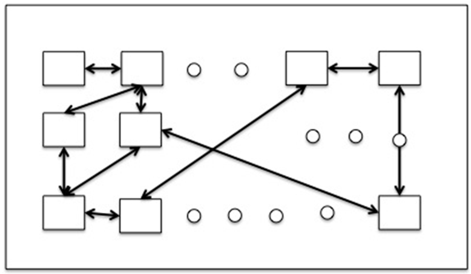
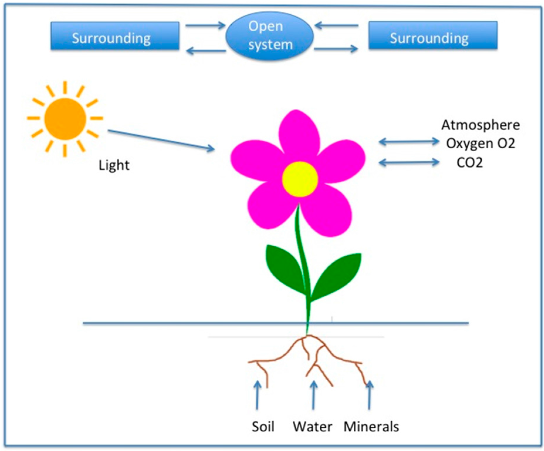
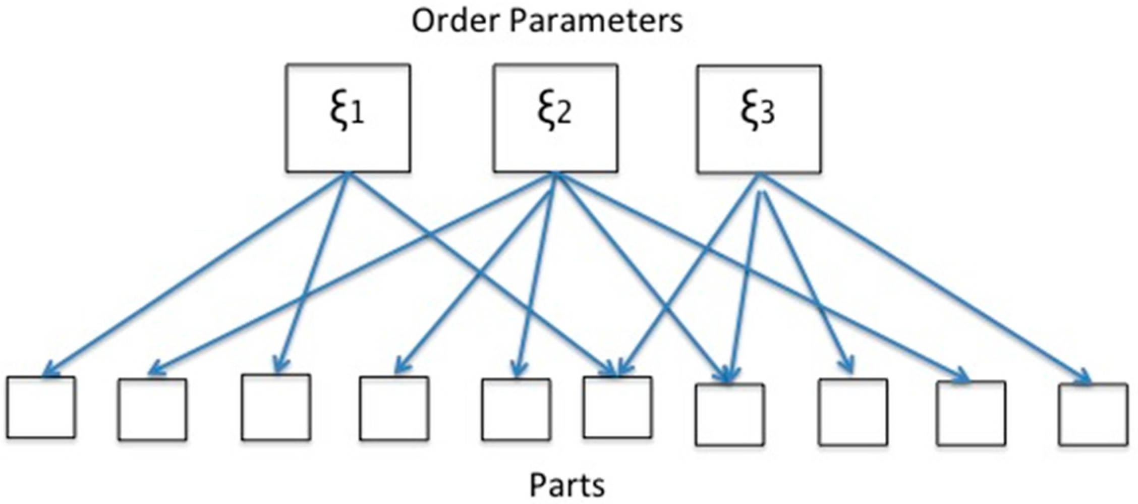
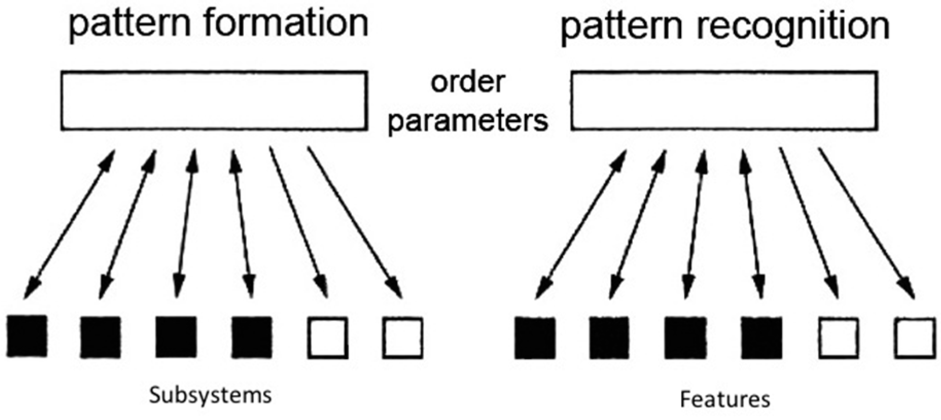
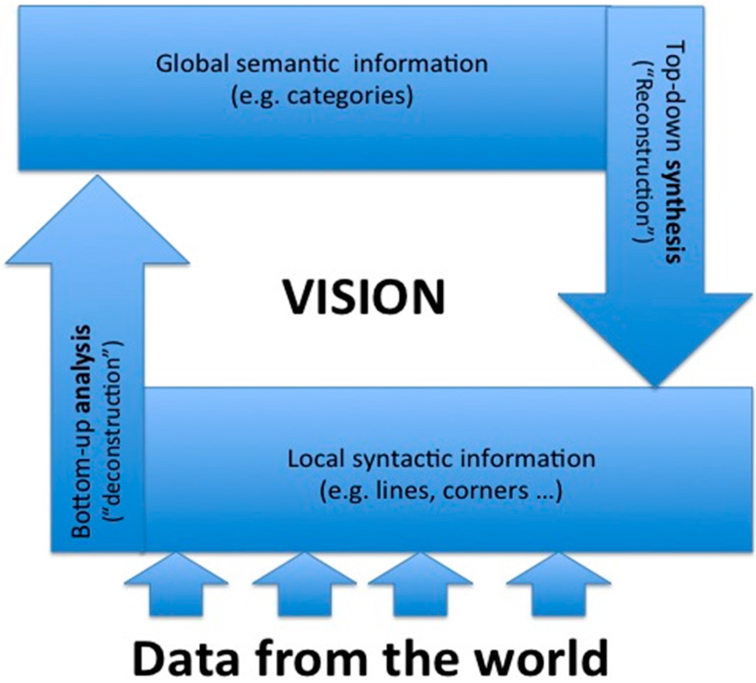
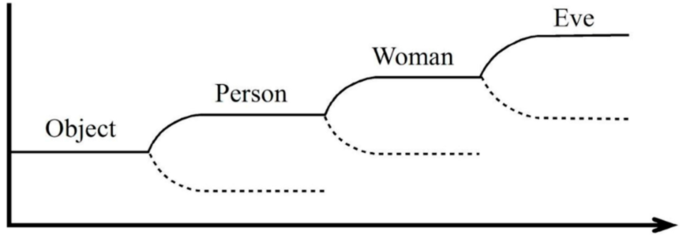
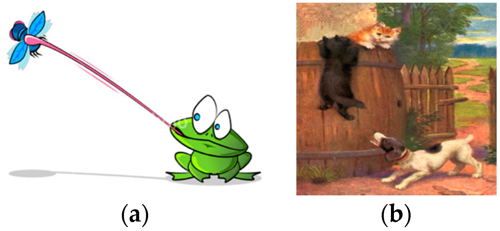
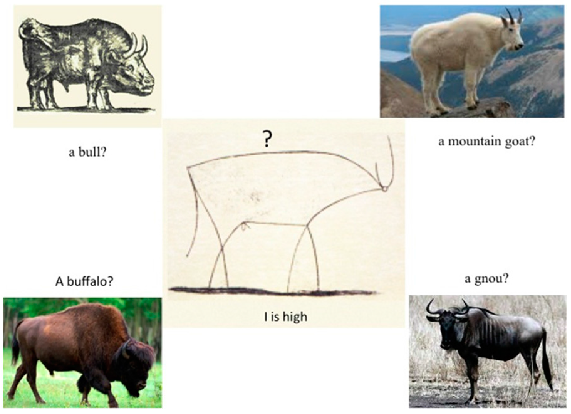
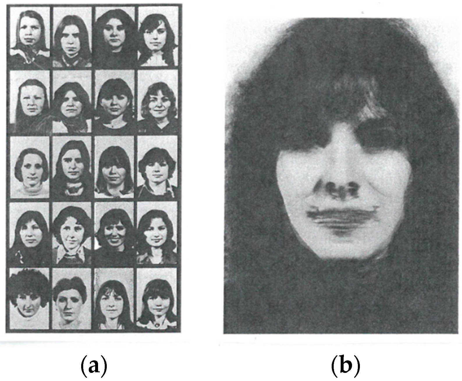
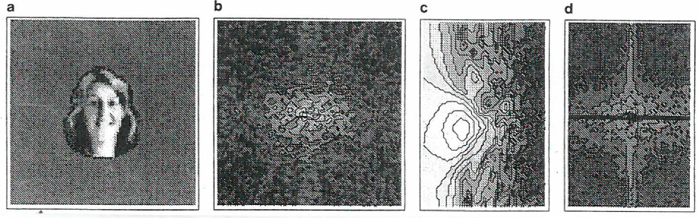
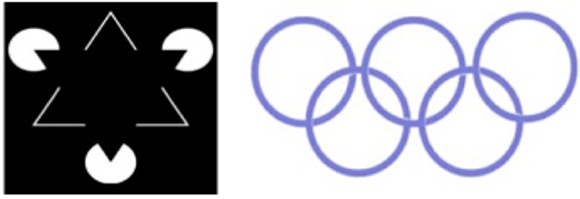
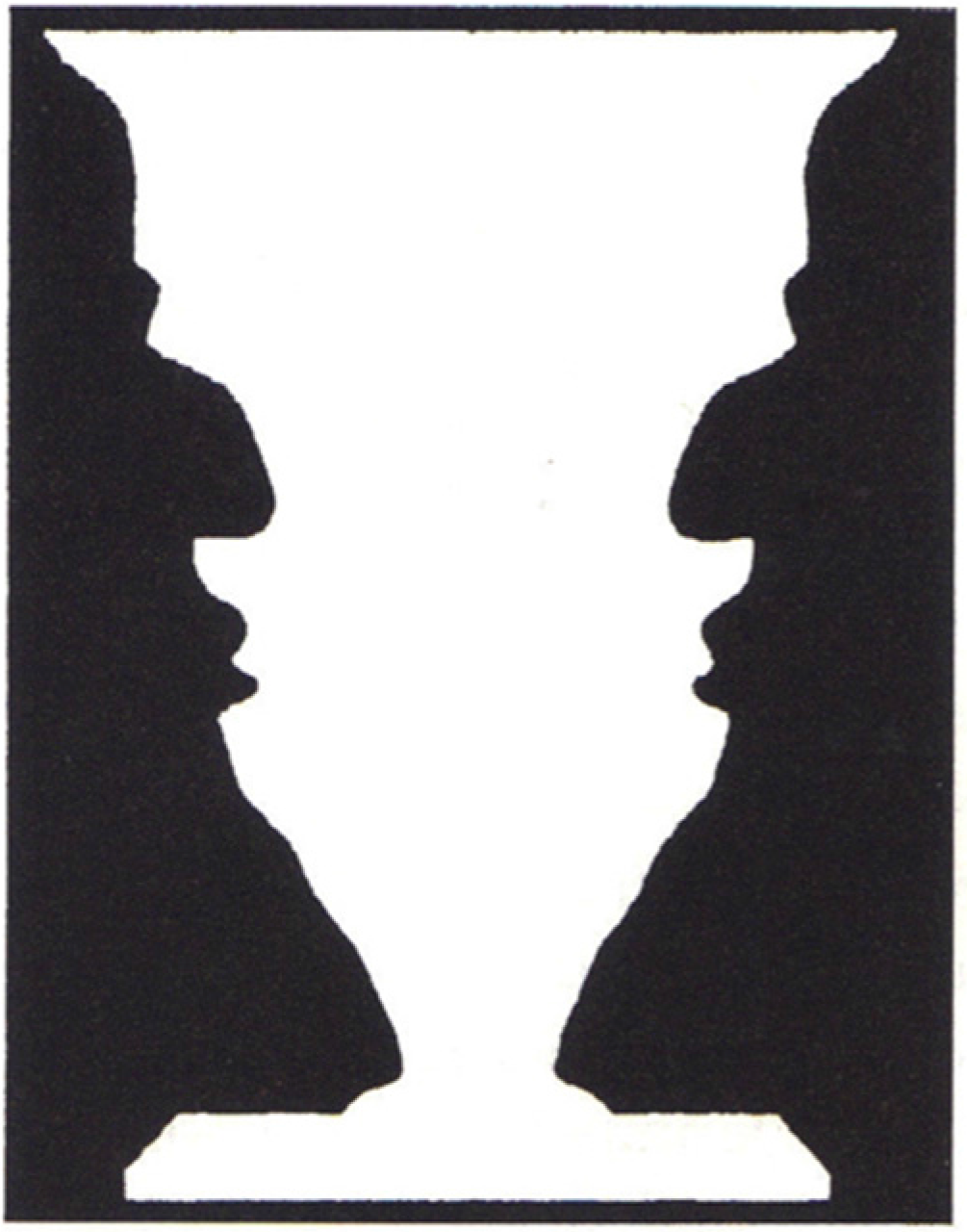
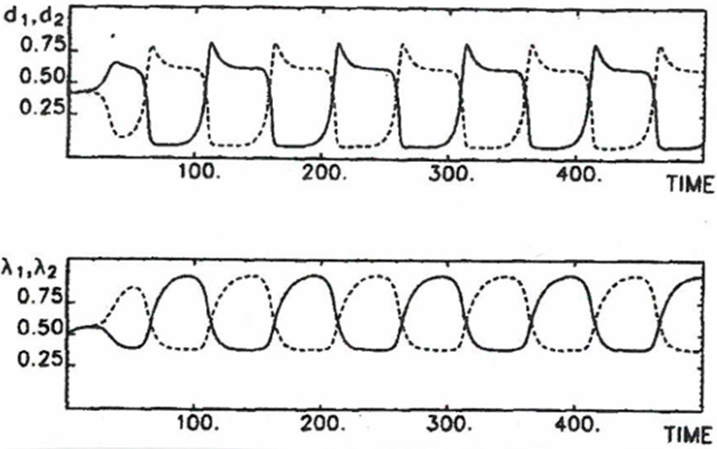
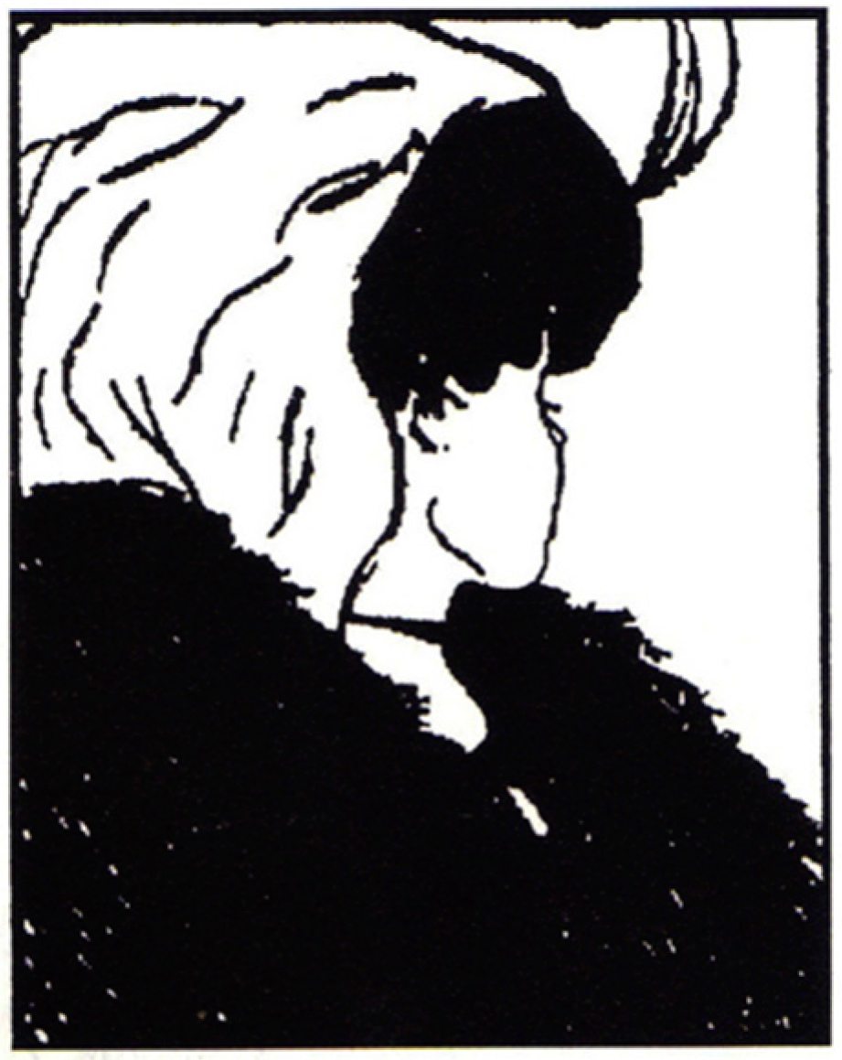
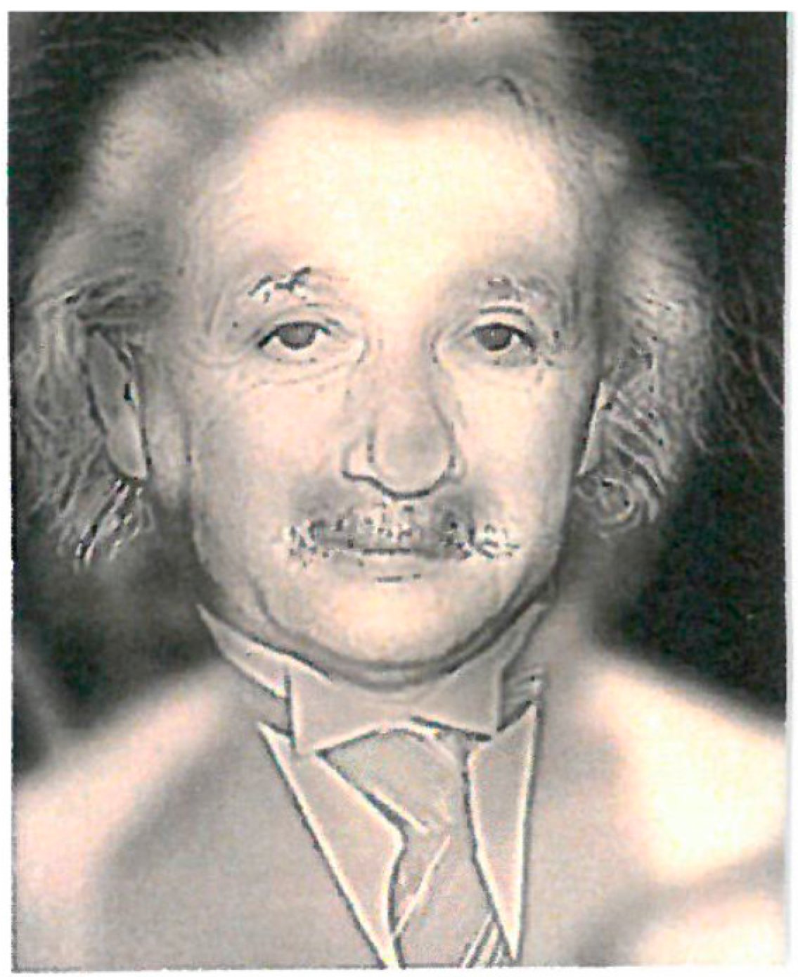
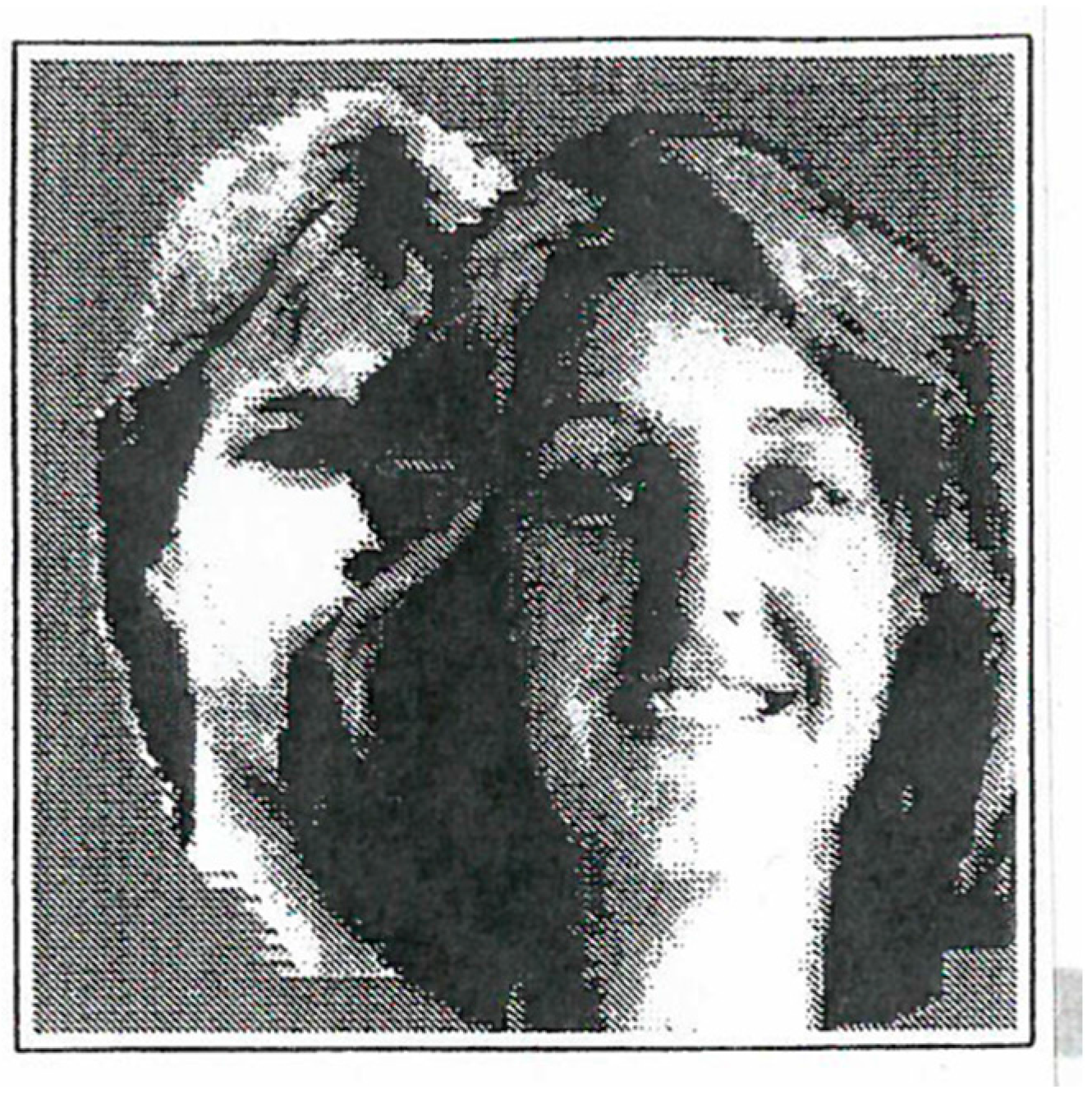
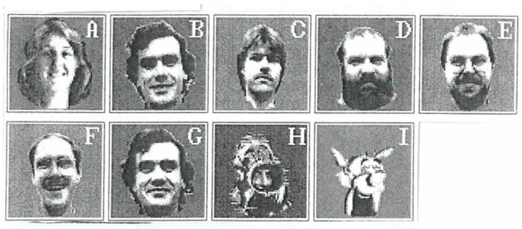
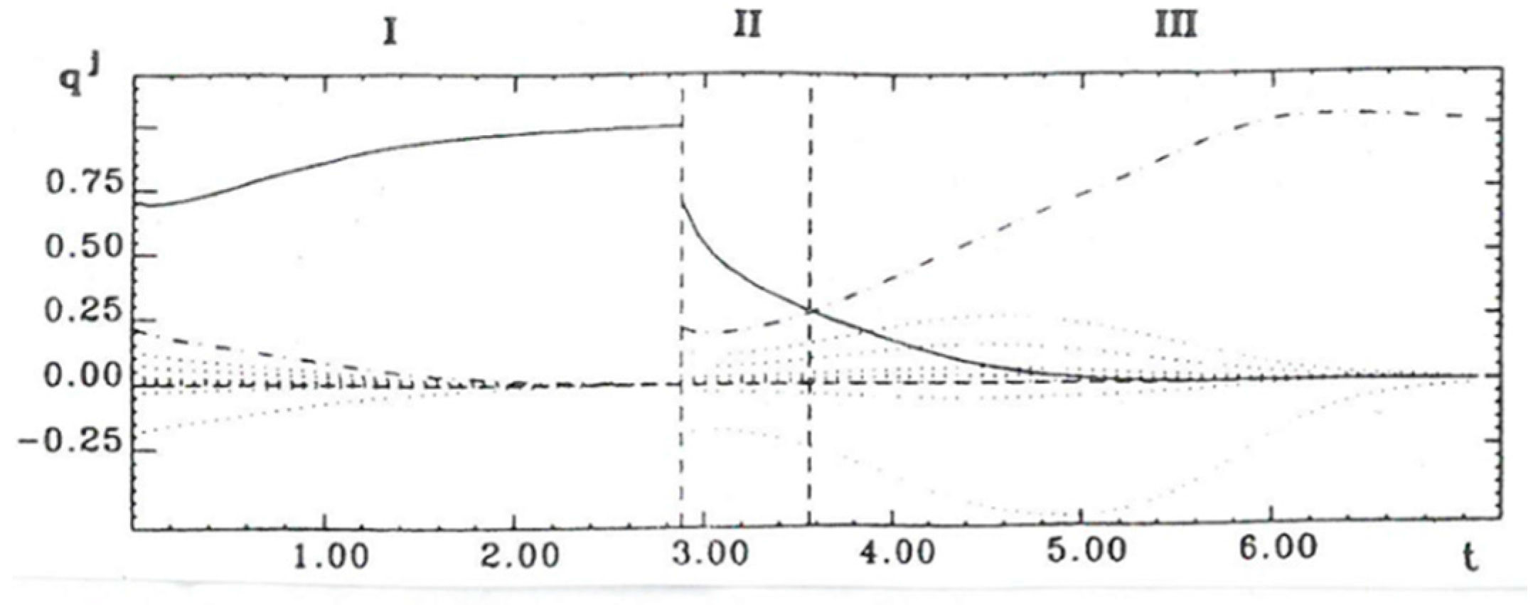
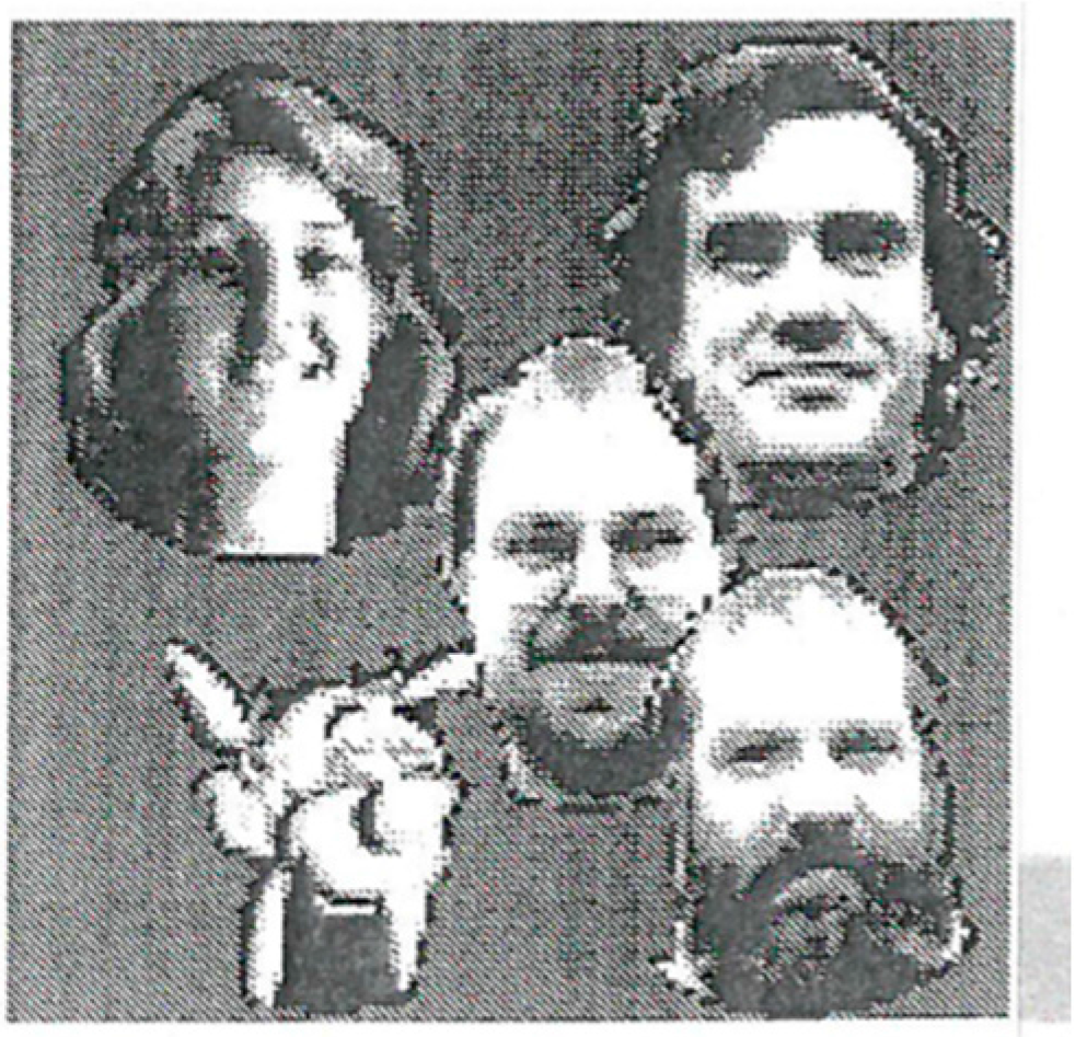
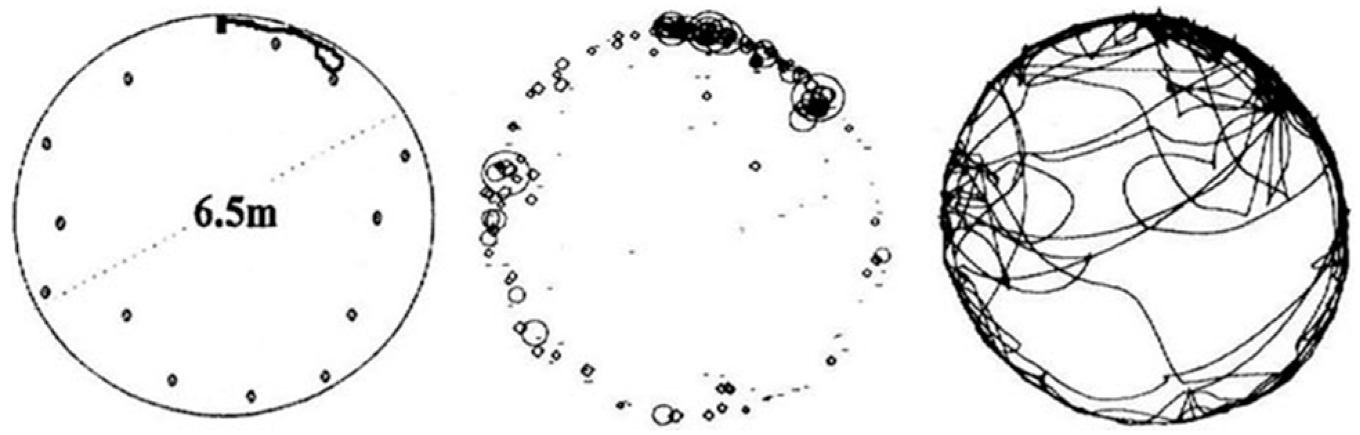
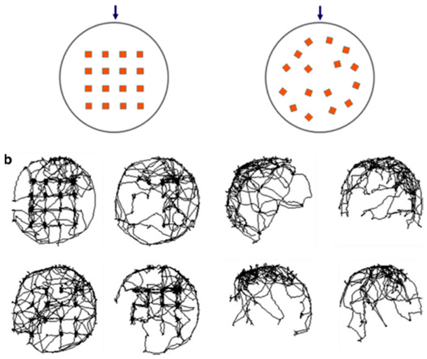
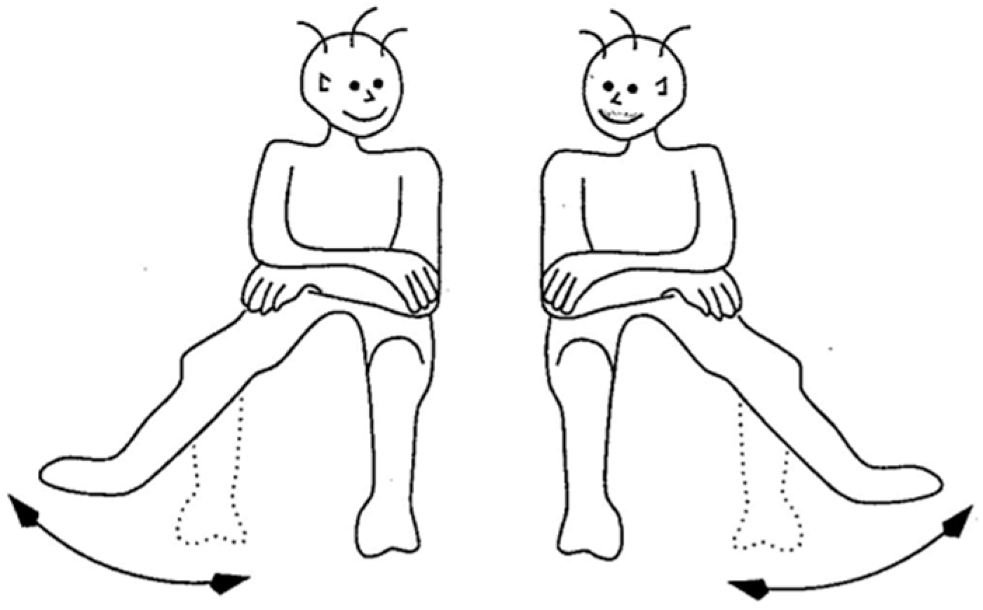
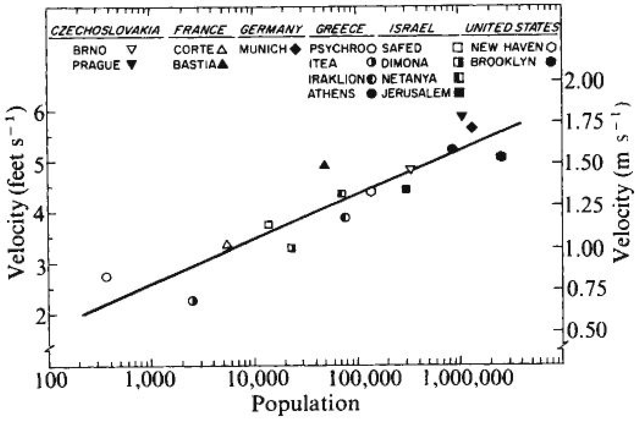
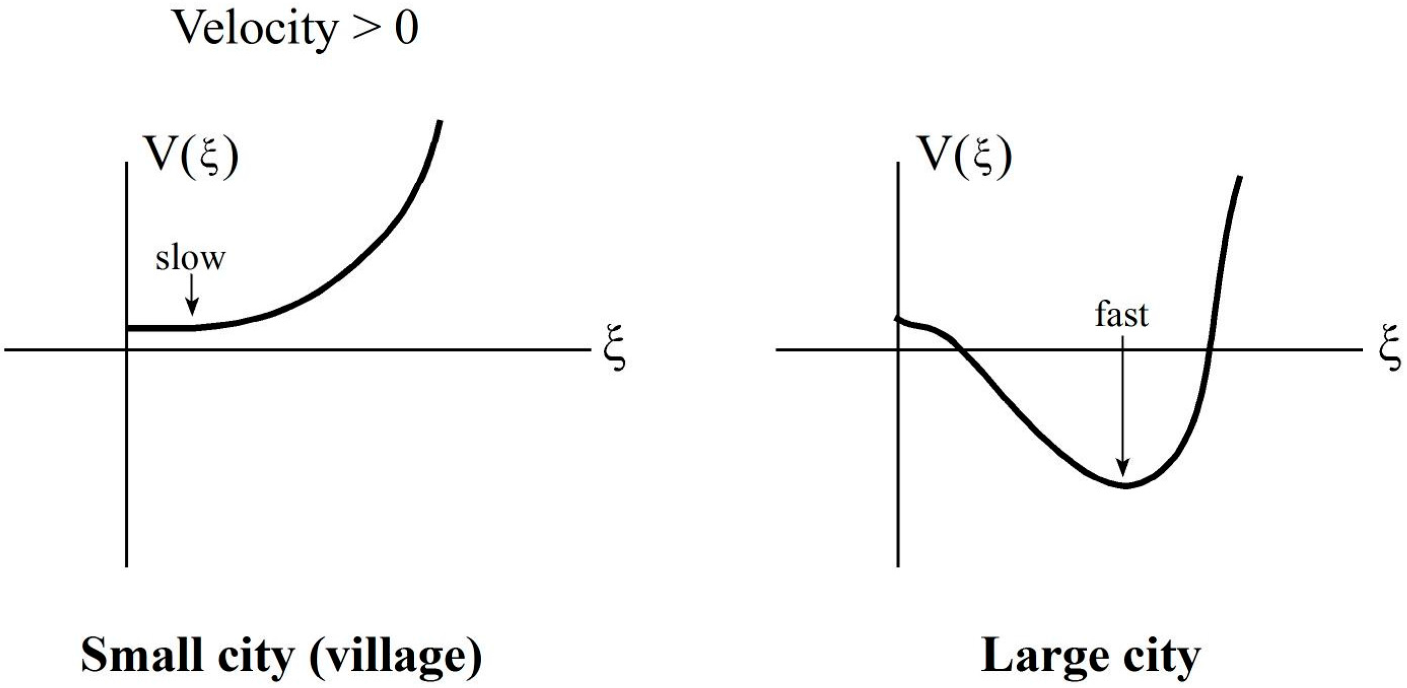
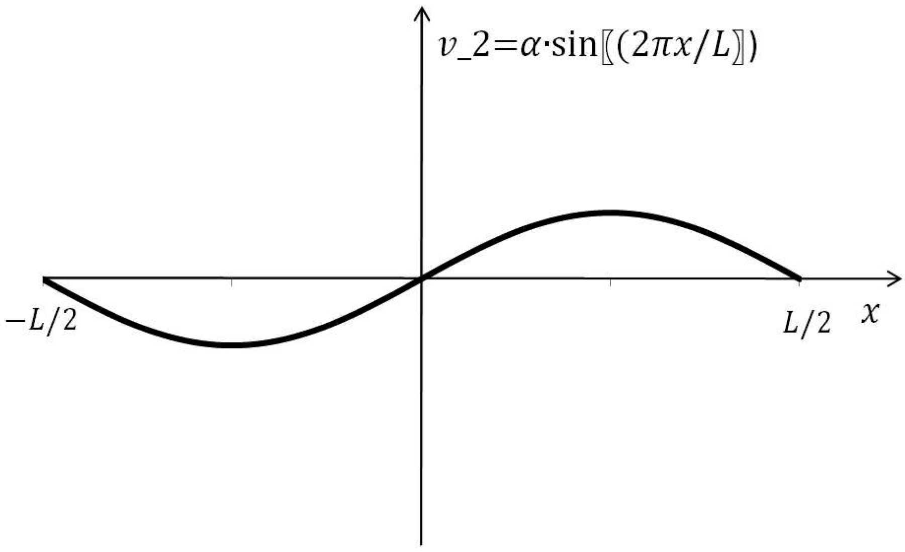
11. Concluding Notes

In our paper we have presented a small cross-section of the large field of information and self-organization from the point of view of algorithmic approaches, in particular inspired by Synergetics and the concept of information adaptation, both dealing with the interplay between microscopic and macroscopic levels. As could be seen, our article has relations to many fields, ranging from neuroscience and neuro-computing to psychophysics, psychology, cognition and urban dynamics. While each of the various fields naturally has a large number of papers on the issues discussed here, we were able to refer to only some key papers, which in turn contain numerous further references not quoted by us. Thus, our paper is not a historical overview and we surely did not quote papers, which would have deserved a quotation and it is likely that we may have overlooked relevant papers. Furthermore, while we have made contact with several fields and effects, we are aware that there are many important effects that we have not treated all. At the microscopic level we did not treat spiking neurons (including their synchronization which may play a role in explaining “binding” [98,99,100], nor the molecular level that, presumably is decisive for memory (cf. Kandel’s [101] early work on Aplysia and Hermissenda). At the macroscopic level we ignored the world of a “freely running” brain with its thoughts, not triggered by external stimuli, as well as the mysterious qualia problem.

References

1. Haken, H. Information and Self-Organization: A Macroscopic Approach to Complex Systems; Springer: Berlin, Germany, 2006. [Google Scholar]
2. Wiener, N. Cybernetics: Or Control and Communication in the Animal and the Machine; MIT Press: Cambridge, MA, USA, 1948. [Google Scholar]
3. Von Foerster, H. Understanding Understanding: Essays on Cybernetics and Cognition; Springer: New York, NY, USA, 2003. [Google Scholar]
4. Von Bertalanffy, L. General System Theory: Foundations, Development, Applications; George Braziller: New York, NY, USA, 1976. [Google Scholar]
5. Haken, H. Synergetic Computers and Cognition; Springer: Berlin, Germany, 2004. [Google Scholar]
6. Haken, H.; Portugali, J. Information Adaptation: The Interplay between Shannonian and Semantic Information in Cognition; Springer: Berlin, Germany, 2015. [Google Scholar]
7. Haken, H. Synergetics: Introduction and Advanced Topics; Springer: Berlin, Germany, 2003. [Google Scholar]
8. Aristotle. Metaphysics; Tufts University Library: Medford, MA, USA, Book 8, section 1045a; pp. 8–10.
9. Paslack, R. Urgeschichte der Selbstorganisation: Zur Archiiologie eines wissenschaftlichen Paradigmas; Friedr. Vieweg & Sohn Verlagsgesellschaft mbH: Braunschweig/Wiesbaden, Germany, 1991. (In German) [Google Scholar]
10. Ashby, W.R. Dynamics of the cerebral cortex automatic development of equilibrium in self-organizing systems. Psychometrika 1947, 12, 135–140. [Google Scholar] [CrossRef]
11. Nicolis, G.; Prigogine, I. Self-Organization in Nonequilibrium Systems: From Dissipative Structures to Order Through Fluctuations; Wiley: New York, NY, USA, 1977. [Google Scholar]
12. Haken, H. Synergetics—An Introduction. Nonequilibrium Phase Transition and Self-Organization in Physics, Chemistry and Biology; Springer: Berlin/Heidelberg, Germany, 1977. [Google Scholar]
13. Pelster, A.; Wunner, G. (Eds.) Self-organization in Complex Systems: The Past, Present, and Future of Synergetics; Springer: Cham, Switzerland, 2016.
14. Haken, H. A NonlinearTheory of Laser Noise and Coherence. Z. Phys. 1964, 181, 96–124. [Google Scholar] [CrossRef]
15. Bénard, H. Les tourbillons cellulaires dans une nappe liquide propageant de la chaleur par convection: En régime permanent. Rev. Gén. Sci. Pures Appl. 1900, 11, 1261–1271, 1309–1328. (In French) [Google Scholar]
16. Shannon, C.E. A Mathematical Theory of Communication. Bell Syst. Tech. J. 1948, 27, 379–423, 623–656. [Google Scholar] [CrossRef]
17. Floridi, L. The Philosophy of Information; Oxford University Press: Oxford, UK, 2011. [Google Scholar]
18. Floridi, L. Semantic Conceptions of Information; Stanford Encyclopedia of Philosophy: Stanford, CA, USA, 2015. [Google Scholar]
19. Graben, P. Pragmatic Information: Historical Exposition and General Overview. Mind Matter 2006, 4, 131–139. [Google Scholar]
20. Hubel, D.H.; Wiesel, T.N. Receptive fields of single neurons in the cat’s striate cortex. J. Physiol. 1959, 148, 574–591. [Google Scholar] [CrossRef] [PubMed]
21. Hubel, D.H.; Wiesel, T.N. Receptive fields, binocular interaction and functional architecture in the cat’s visual cortex. J. Physiol. 1962, 160, 106–154. [Google Scholar] [CrossRef] [PubMed]
22. Hubel, D.H.; Wiesel, T.N. Receptive fields and functional architecture in two nonstriate visual areas (18 and 19) of the cat. J. Neurophysiol. 1965, 28, 229–289. [Google Scholar] [PubMed]
23. Livingstone, M.S. Vision and Art: The Biology of Seeing; Harry N. Abrams: New York, NY, USA, 2002. [Google Scholar]
24. Freiwald, W.A.; Tsao, D.Y. Functional Compartmentalization and generalization Within the Macaque Face-Processing System. Science 2010, 330, 845–851. [Google Scholar] [CrossRef] [PubMed]
25. Kandel, E. The Age of Insight: The Quest to Understand the Unconscious in Art, Mind, and Brain, from Vienna 1900 to the Present; Random House: New York, NY, USA, 2012. [Google Scholar]
26. Latimer, K.W.; Yates, J.L.; Meister, M.L.R.; Huk, A.C.; Pillow, J.W. Single-trial spike trains in parietal cortex reveal discrete steps during decision-making. Science 2015, 349, 184–187. [Google Scholar] [CrossRef] [PubMed]
27. Wilson, R.A.; Foglia, L. Embodied Cognition; Stanford Encyclopedia of Philosophy: Stanford, CA, USA, 2011. [Google Scholar]
28. Klyubin, A.S.; Polani, D.; Nehaniv, C.L. Empowerment: A Universal Agent-Centric Measure of Control. In Proceedings of 2005 IEEE Congress on Evolutionary Computation, Edinburgh, Scotland, 5 September 2005.
29. Maturana, H.R.; Lettvin, J.Y.; McCulloch, W.S.; Pitts, W.H. Anatomy and Physiology of Vision in the Frog (Rana pipiens). J. Gen. Physiol. 1960, 43, 129–175. [Google Scholar] [CrossRef] [PubMed]
30. Haken, H.; Portugali, J. The face of the city is its information. J. Environ. Psychol. 2003, 23, 382–405. [Google Scholar] [CrossRef]
31. Portugali, J. Complexity, Cognition and the City; Springer: Berlin, Germany, 2011. [Google Scholar]
32. Haken, H.; Kelso, J.A.S.; Bunz, H. A theoretical model of phase transitions in human hand movements. Biol. Cybern. 1985, 51, 347–356. [Google Scholar] [CrossRef] [PubMed]
33. Jaynes, E.T. Information Theory and Statistical Mechanics. Phys. Rev. 1957, 106. [Google Scholar] [CrossRef]
34. Jaynes, E.T. Information Theory and Statistical Mechanics. II. Phys. Rev. 1957, 108, 171. [Google Scholar] [CrossRef]
35. Guckenheimer, J.; Holmes, P. Nonlinear Oscillations, Dynamical Systems, and Bifurcations of Vector Fields, 7th ed.; Springer: New York, NY, USA, 2002. [Google Scholar]
36. Risken, H. Distribution-and correlation functions for a laser amplitude. Z. Phys. 1965, 186, 85–98. [Google Scholar] [CrossRef]
37. De Giorgio, V.; Scully, M. Analogy between the Laser Threshold Region and a Second-Order Phase Transition. Phys. Rev. A 1970, 2, 1170. [Google Scholar] [CrossRef]
38. Graham, R.; Haken, H. Laserlight—First example of a second order phase transition far from thermal equilibrium. Z. Phys. 1970, 237, 31–46. [Google Scholar] [CrossRef]
39. Friston, K. A free energy principle for biological systems. Entropy 2012, 14, 2100–2121. [Google Scholar]
40. Gibson, J.J. The Ecological Approach to Visual Perception; Houghton-Mifflin: Boston, MA, USA, 1979. [Google Scholar]
41. Haken, H.; Portugali, J. Synergetics, Inter-representation networks and cognitive maps. In GeoJournal Library; Kluwer Academic Publishers: Dordrecht, The Netherlands, 1996; pp. 45–67. [Google Scholar]
42. Haken, H. Principles of Brain Functioning: A Synergetic Approach to Brain Activity, Behavior and Cognition; Springer: Berlin/Heidelberg, Germany, 1996. [Google Scholar]
43. Atmanspacher, H.; Demmel, G. Methodological issues in the study of complex systems. In Reproducibility: Principles, Problems, Practices, Prospects; Wiley: New York, NY, USA, 2015; pp. 233–250. [Google Scholar]
44. Atmanspacher, H.; Scheingraber, H. Pragmatic information and dynamical instabilities in a multimode continuous-wave dye laser. Can. J. Phys. 1990, 68, 728–737. [Google Scholar] [CrossRef]
45. Freeman, W.J. Origin, structure, and role of background EEG activity. Part 3. Neural frame classification. Clin. Neurophys. 2005, 116, 1118–1129. [Google Scholar] [CrossRef] [PubMed]
46. Haken, H. Brain dynamics; Springer: Berlin/Heidelberg, Germany, 2002. [Google Scholar]
47. Friston, K.; Adams, R.A.; Perrinet, L.; Breakspeare, M. Perceptions as hypotheses: Saccades as experiments. Front. Psychol. 2012, 3. [Google Scholar] [CrossRef] [PubMed]
48. Anselmi, F.; Leibo, J.Z.; Rosasco, L.; Mutch, J.; Tacchetti, A.; Poggio, T. Unsupervised learning of invariant representations with low sample complexity: the magic of sensory cortex or a new framework for machine learning? 2014; arXiv:1311.4158v5. [Google Scholar]
49. Haken, H. Synergetics as a tool for the Conceptionalization and Mathematization of Cognition and Behaviour—How Far can we go? In Synergetics of Cognition; Haken, H., Stadler, M., Eds.; Springer: Berlin, Germany, 1990; Volume 45, pp. 2–31. [Google Scholar]
50. Rentschler, I.; Herzberger, B.; Epstein, D. Beauty and the Brain: Biological Aspects of Aesthetics; Birkhäuser: Basel, Switzerland, 1988. [Google Scholar]
51. Fuchs, A.; Haken, H. Pattern Recognition and Associative Memory as Dynamical Processes in a Synergetic System. Biol. Cybern. 1988, 60, 17–22. [Google Scholar] [CrossRef] [PubMed]
52. Köhler, W. Dynamics in Psychology; Liveright: New York, NY, USA, 1940. [Google Scholar]
53. Wertheimer, M. Untersuchungen zur Lehre von der Gestalt, I: Prinzipielle Bemerkungen [Investigations in Gestalt Theory: I. The general theoretical situation]. Psychol. Forsch. 1922, 1, 47–58. (In German) [Google Scholar] [CrossRef]
54. Wertheimer, M. Untersuchungen zur Lehre von der Gestalt, II. [Investigations In Gestalt Theory: II. Laws of organization in perceptual forms]. Psychol. Forsch. 1923, 4, 301–350. (In German) [Google Scholar] [CrossRef]
55. Shephard, R.M.; Chipman, S. Second-order Isomorphism of Internal Representations: Shapes of States. Cogn. Psychol. 1970, 1, 1–17. [Google Scholar] [CrossRef]
56. Shephard, R.M.; Metzler, J. Mental Rotation of Three-dimensional Objects. Science 1971, 171, 701–703. [Google Scholar] [CrossRef]
57. Kosslyn, S.M. Image and Mind; Harvard University Press: Cambridge, MA, USA, 1980. [Google Scholar]
58. Pylyshyn, Z.W. Computation and Cognition: Toward a Foundation for Cognitive Science; MIT Press: Cambridge MA, USA, 1984. [Google Scholar]
59. Kosslyn, S.M.; Ball, T.M.; Reiser, B.J. Visual images preserve metric spatial information: Evidence from studies of image scanning. J. Exp. Psychol. Hum. Percept. Perform. 1978, 4, 47–60. [Google Scholar] [CrossRef] [PubMed]
60. Ditzinger, T.; Haken, H. The impact of fluctuations on the recognition of ambiguous patterns. Biol. Cybern. 1990, 63, 453–456. [Google Scholar] [CrossRef] [PubMed]
61. Ditzinger, T.; Haken, H. Oscillations in the perception of ambiguous patterns. Biol. Cybern. 1989, 61, 279–287. [Google Scholar] [CrossRef]
62. Oliva, A.; Schyns, P.F. Coarse Blobs or Fine Edges? Evidence That Information Diagnosticity Changes the Perception of Complex Visual Stimuli. Cogn. Psychol. 1997, 34, 72–107. [Google Scholar] [CrossRef] [PubMed]
63. Huang, G.T. Hybrid images: Now you see them. New Sci. 2007, 2597, 35–37. [Google Scholar] [CrossRef]
64. Findlay, J.; Walker, R. Human saccadic eye movements. Scholarpedia 2012, 7, 5095. [Google Scholar] [CrossRef]
65. Van der Stigchel, S.; Nijboer, T.C.W. The global effect: what determines where the eyes land? J. Eye Mov. Res. 2011, 4, 1–13. [Google Scholar]
66. Findlay, J.M.; Blythe, H.I. Saccade target selection: do distractors affect saccade accuracy? Vis. Res. 2009, 49, 1267–1274. [Google Scholar] [CrossRef] [PubMed]
67. Hepp, K.; Suzuki, Y.; Straumann, D.; Hess, B.J.M. On the 3-dimensional rapid eye movement generator in monkey. In Information Processing Underlying Gaze Control; Delgadio-Garcia, J.M., Godeaux, M., Vidal, P.P., Eds.; Pergamon: London, UK, 1994; pp. 65–74. [Google Scholar]
68. Heinzle, J.; Hepp, K.; Martin, K.A.C. A Biological Realistic Cortical Model of Eye Movement Control in Reading. Psychol. Rev. 2010, 117, 808–830. [Google Scholar] [CrossRef] [PubMed]
69. Yarbus, A.L. Eye Movements and Vision; Plenum Press: New York, NY, USA, 1967. [Google Scholar]
70. Hinton, G. E. Where do features come from? Cogn. Sci. 2014, 38, 1078–1101. [Google Scholar] [CrossRef] [PubMed]
71. Kullback, S. Letter to the Editor: The Kullback–Leibler distance. Am. Stat. 1987, 41, 340–341. [Google Scholar]
72. Pomplun, M.; Ritter, H.; Velichkovsky, B. Disambiguating complex visual information: Towards communication of personal views of a scene. Perception 1996, 25, 931–948. [Google Scholar] [CrossRef] [PubMed]
73. Henderson, J.M. Human gaze control during real-world scene perception. Trends Cogn. Sci. 2003, 7, 498–504. [Google Scholar] [CrossRef] [PubMed]
74. Coco, M.I.; Keller, F. Interplaying mechanisms of visual guidance in naturalistic language production. Cogn. Process. 2015, 16, 131–150. [Google Scholar] [CrossRef] [PubMed]
75. Golani, I.; Einat, C.; Tchernichovsky, O.; Teitelboum, P. Keeping the body straight in the locomotion of normal and dopamine stimulant treated rats. J. Motor Behav. 1997, 29, 99–112. [Google Scholar] [CrossRef] [PubMed]
76. Golani, I.; Kafkafi, N.; Drai, D. Phenotyping stereotypic behaviour: collective variables, range of variation and predictability. Appl. Anim. Behav. Sci. 1999, 65, 191–220. [Google Scholar] [CrossRef]
77. Yaski, O.; Portugali, J.; Eilam, D. City rats: Insight from rat spatial behavior into human cognition in urban environments. Anim. Cogn. 2011, 14, 655–663. [Google Scholar] [CrossRef] [PubMed]
78. Yaski, O.; Portugali, J.; Eilam, D. Arena geometry and path shape: When rats travel in straight or in circuitous paths? Behav. Brain Res. 2011, 225, 449–454. [Google Scholar] [CrossRef] [PubMed]
79. Gordon, G.; Fonio, E.; Ahissar, E. Emergent Exploration via Novelty Management. J. Neurosci. 2014, 34, 12646–12661. [Google Scholar] [CrossRef] [PubMed]
80. Schmidt, R.C.; Carello, C.; Turvey, M.T. Phase transitions and critical fluctuations in the visual coordination of rhythmic movements between people. J. Exp. Psychol. Hum. Percept. Perform. 1990, 16, 227–247. [Google Scholar] [CrossRef] [PubMed]
81. Bornstein, M.H.; Bornstein, H.G. The pace of life. Nature 1976, 259, 557–559. [Google Scholar] [CrossRef]
82. Walmsley, D.J.; Lewis, G.J. The pace of pedestrian flows in cities. Environ. Behav. 1989, 21, 123–150. [Google Scholar] [CrossRef]
83. Levine, R.; Norenzayan, A. The Pace of Life in 31 Countries. J. Cross Cult. Psychol. 1999, 30, 178–205. [Google Scholar] [CrossRef]
84. Bettencourt, L.M.A.; Lobo, J.; Helbing, D.; Kuhnert, C.; West, G.B. Growth, innovation, scaling, and the pace of life in cities. Proc. Natl. Acad. Sci. 2007, 104, 7301–7306. [Google Scholar] [CrossRef] [PubMed]
85. Gigerenzer, G. Simply Rational: Decision Making in the Real World; Oxford University Press: New York, NY, USA, 2015. [Google Scholar]
86. Milgram, S. The Experience of Living in Cities. Science 1970, 167, 1461–1468. [Google Scholar] [CrossRef] [PubMed]
87. Tononi, G. Integrated information theory of consciousness: An updated account. Arch. Ital. Biol. 2012, 150, 56–90. [Google Scholar] [PubMed]
88. Dehaene, S. Consciousness and the Brain; Viking Press: New York, NY, USA, 2014. [Google Scholar]
89. Crick, F.; Koch, C. Some Reflections on Visual Awareness. Cold Spring Harb. Symp. Quantative Biol. 1990, 55, 953–962. [Google Scholar] [CrossRef]
90. Crick, F.; Koch, C. Toward a neurobiological theory of consciousness. Semin. Neurosci. 1990, 2, 263–275. [Google Scholar]
91. Wheatstone, C. Contributions to the physiology of vision.—Part the First. On some remarkable, and hitherto unobserved, phenomena of binocular vision. Philos. Trans. R. Soc. Lond. 1838, 128, 371–394. [Google Scholar] [CrossRef]
92. Leopold, D.A.; Logothetis, N.K. Multistable phenomena: changing views in perception. Trends Cogn. Sci. 1999, 3, 254–264. [Google Scholar] [CrossRef]
93. Borsellino, A.; De Marco, A.; Allazetta, A.; Rinesi, S.; Bartolini, B. Reversal time distribution in the perception of visual ambiguous stimuli. Kybernetik 1972, 10, 139–144. [Google Scholar] [CrossRef] [PubMed]
94. Del Cul, A.; Baillet, S.; Dehaene, S. Brain dynamics underlying the nonlinear threshold for Access to Consciousness. PLoS Biol. 2007, 5. [Google Scholar] [CrossRef] [PubMed] [Green Version]
95. Haken, H. Advanced Synergetics; Springer: Berlin/Heidelberg, Germany; New York, NY, USA, 1983. [Google Scholar]
96. Haken, H. Pattern formation and pattern recognition—An attempt at a synthesis. In Pattern Formation by Dynamic Systems and Pattern Recognition; Haken, H., Ed.; Springer: Berlin/Heidelberg, Germany, 1979; pp. 2–13. [Google Scholar]
97. Dehaene, S.; Naccache, L. Towards a cognitive neuroscience of consciousness. Basic evidence and workspace frame work. Cognition 2001, 79, 1–37. [Google Scholar]
98. Gray, C.M.; Singer, W. Stimulus-dependent neuronal oscillations in the cat visual cortex area 17. IBRO Abstr. Neurosci. Lett. Suppl. 1987, 22, 1301P. [Google Scholar]
99. Gray, C.M. The temporal correlation hypothesis: Still alive and well. Neuron 1999, 24, 31–47. [Google Scholar] [CrossRef]
100. Singer, W. Neural synchrony: A versatile code for the definition of relation? Neuron 1999, 24, 49–65. [Google Scholar] [CrossRef]
101. Kandel, E.R. Behavioral Biology of Aplysia: A Contribution to the Comparative Study of Epistobranch Molluscs; W.H. Freeman: San Francisco, CA, USA, 1979. [Google Scholar]
102. Busemeyer, J.R.; Bruza, P.D. Quantum Models of Cognition and Decision; University Press: Cambridge, UK, 2012. [Google Scholar]
103. Ackley, D.H.; Hinton, G.E.; Sejnowski, T.J. Cogn. Sci. 1985, 9, 147–169.
Figure 1. A complex selforganizing system is composed of parts, elements, components, units, etc. Its network of interactions serves for exchange of matter, energy, and information. The open circles stand for further parts.
Entropy 18 00197 g001
Figure 2. Scheme of an open system: A plant with its surroundings.
Entropy 18 00197 g002
Figure 3. (a) and (b) Convection cells in rectangular vessel; (c) Convection cells in circular vessel.
Entropy 18 00197 g003
Figure 4. The behavior of many parts (bottom) is governed (“enslaved”) by very few order parameters (top). Note that in contrast to Figure 1 here the parts are no more connected by lines because in our formalism the direct interactions are replaced by the lines illustrating the slaving principle.
Entropy 18 00197 g004
Figure 5. Analogy between pattern formation (left) and pattern recognition (right). In pattern formation the subsystems are enslaved by the order parameters (OPs); in the case of pattern recognition it is the features that are enslaved by OPs. Based on [5] (p. 37), Figure 5.2. The unfilled squares symbolize parts that are not yet in the ordered state but will be pulled into it (“enslaved”).
Entropy 18 00197 g005
Figure 6. Schematic illustration of visual perception.
Entropy 18 00197 g006
Figure 7. Schematic (non-mathematical) description of the approaching lady (abscissa = amount of data vs. ordinate = recognized category/pattern). The broken line indicates the other dismissed options. The saltatory dynamics in Figure 7 are remarkably similar to empirical results that show similar (stepping) dynamics during evidence accumulations in the parietal cortex [26].
Entropy 18 00197 g007
Figure 8. (a) Frog’s reflective action; (b) Cat’s and dog’s perceptive action.
Entropy 18 00197 g008
Figure 9. If you are not familiar with Picasso’s Bull (Center), you might interpret it as a bull, mountain goat, buffalo a gnou or another similar animal. Source: [6], Figure 2.2.
Entropy 18 00197 g009
Figure 10. Phase transition in finger movement coordination.
Entropy 18 00197 g010
Figure 11. An illustration of Equation (114). This figure was originally created by H. Daucher 1979 and served as example of the formation of templates by statistical learning as presented by I. Eibl-Eibesfeld in Rentschler et al. [50]. Reproduced with permission from [50].
Entropy 18 00197 g011
Figure 12. The various transformations applied to a face. From left to right: (a) the original pattern in the (x,y) plane; (b) the absolute value of its Fourier transform in the ( k x , i k y ) plane. Light shading corresponds to large values of | c ( k z , i k y ) | ; (c) the logarithmic map; (d) the absolute square of the Fourier transform of pattern (c). From Fuchs and Haken [51].
Entropy 18 00197 g012
Figure 13. As in Figure 12 but with all transformations performed simultaneously. From [51]. Note that Figure 13 right coincides with Figure 12d.
Entropy 18 00197 g013
Figure 14. (Left): The Kaniza triangle illusion. (Right): The “Olympic rings” illusion. See discussion in [6].
Entropy 18 00197 g014
Figure 15. Vase or Faces?
Entropy 18 00197 g015
Figure 16. Order parameters and attention parameters vs. time. Source: [61].
Entropy 18 00197 g016
Figure 17. Old or Young woman?
Entropy 18 00197 g017
Figure 18. Example of a hybrid image: Einstein/Monroe. Reproduced with permission from [63].
Entropy 18 00197 g018
Figure 19. A complex scene to be recognized by the synergetic computer. From [51].
Entropy 18 00197 g019
Figure 20. The faces that are stored as the prototype patterns. The letters encode the names or identify the figures.In addition to the faces other figures were also included to check how the synergetic computer responds and what properties it displays when recognizing these patterns. From [51].
Entropy 18 00197 g020
Figure 21. Time evolution of the order parameters ξ 1 (woman), ξ 2 (man) corresponding to Figure 19. When ξ 1 has come close to unity, the attention parameter for the woman is switched to zero and then a new time evolution sets in as shown, eventually indicating that the man has been recognized. From [51].
Entropy 18 00197 g021
Figure 22. Example of a scene composed of five faces recognized by the computer using the procedure described in the text. From [51].
Entropy 18 00197 g022
Figure 23. A typical exploratory behavior experiment of a rat. Left: Line tracing the rat’s forward and backward movements in the first exploratory excursion. Right: Line tracing the rat’s movement in all progressing episodes. Center: The rat’s constructed space (arena): stopping locations (bases) with dwell time represented by circles’ size. Reproduced with permission from [75,76].
Entropy 18 00197 g023
Figure 24. Paths of progression of rats in grid versus irregular layouts.
Entropy 18 00197 g024
Figure 25. Paths of progression of four rats in grid and random layouts, during the 20 min of testing. The arrows indicate the starting point at which the rats were placed in the arena at the beginning of exploration.
Entropy 18 00197 g025
Figure 26. Upper part: potential vs order parameter. Left, “slow” motion case. Right “fast” motion case. Lower part: movement patterns of index fingers corresponding to upper part of Figure after Haken et al. [32].
Entropy 18 00197 g026
Figure 27. Coordination between legs’ movement.
Entropy 18 00197 g027
Figure 28. The Bornsteins’ correlation between population size of cities and walking speed of pedestrians in these cities.
Entropy 18 00197 g028
Figure 29. Potential V versus parameter ξ (velocity).
Entropy 18 00197 g029