Empirical Laws and Foreseeing the Future of Technological Progress

Abstract

The Moore’s law (ML) is one of many empirical expressions that is used to characterize natural and artificial phenomena. The ML addresses technological progress and is expected to predict future trends. Yet, the “art” of predicting is often confused with the accurate fitting of trendlines to past events. Presently, data-series of multiple sources are available for scientific and computational processing. The data can be described by means of mathematical expressions that, in some cases, follow simple expressions and empirical laws. However, the extrapolation toward the future is considered with skepticism by the scientific community, particularly in the case of phenomena involving complex behavior. This paper addresses these issues in the light of entropy and pseudo-state space. The statistical and dynamical techniques lead to a more assertive perspective on the adoption of a given candidate law.

1. Introduction

In 1965, the physical chemist Gordon E. Moore, co-founder of both Intel and Fairchild Semiconductor, wrote an article for the 35th anniversary issue of Electronics magazine about the evolution of the semiconductor industry [1]. Moore noted that the complexity of minimum cost semiconductor components had doubled per year since 1959, the date of production of the first chip [2]. Such exponential increase in the number of components on an integrated circuit became later the so-called Moore’s law (ML), predicting that the number of components that could be placed on a chip could be expected to double every year, and that such trend would continue for the foreseeable future [3,4,5].

Moore revised his first prediction in the year 1980 [6], stating that the exponential increase could approximately double every two years, rather than every year [6]. Since 1980, ML had successive revisions and reinterpretations that, in fact, ensured its survival. At the beginning of the 1980’s, ML meant “the number of transistors on a chip would double every 18 months”, in 1990 it became interpreted as “doubling of microprocessor power every 18 months”, and in the 1990’s it was reformulated to enunciate that “computing power at fixed cost would double every 18 months” [2], just to cite a few formulations. This apparent weakness of the empirical ML became its main strength, and made the law seem accurate until now [3].

The ML disseminated beyond semiconductor and computer technologies [3,7]. In a broader sense, the ML refers to the perceived increase in the rate of technological development throughout history, suggesting faster and more profound changes in the future, possibly accompanied by underlying economic, cultural and social changes [8,9,10,11,12,13].

Given the apparent ubiquity of the ML (here interpreted in the broad sense of “exponential growth”) [13,14,15], simple questions can be raised: Does ML describe technological development accurately? Can it be used for reliable forecasting?

The so-called exponential growth should be understood as an approximate empirical model for real data. During more than two decades, several authors foresaw the end of ML, arguing that technological limits were close [5,16,17]. Others defended that ML would survive for many years, as they envisaged the emergence of a new paradigm that could enlarge dramatically the existent technological bounds. Within such paradigm novel technologies would became available, such as quantum devices [18,19,20], biological [21], molecular [22], or heterotic computing [23]. Those technologies would thereafter keep ML alive.

Whatever one’s opinion, either forward-looking, or conservative, we should note that forecasting technological evolution for many years ahead from now is difficult. Technological innovation means by definition something that is new and, therefore, may be inherently unpredictable [24]. However, even a rough knowledge about technological evolution could be invaluable for helping decision makers to delineate adequate policies, seeking sustainability and improvement of individual and collective living [25,26].

In this paper we seek to contribute for the discussion of some the questions raised above. We illustrate our scheme with real data representative of technological progress in time. In that perspective, we adopt 4 performance indices: (i) the world inflation-adjusted gross domestic product (GDP), measured in 2010 billions of U.S. dollars; (ii) the performance of the most powerful supercomputers (PPS), expressed in tera FLOPS (floating-point operations per second); (iii) the number of transistors per microprocessor (TPM), and (iv) the number of U.S. patents granted (USP). Obviously, other data-series may be candidate for assessing the technological evolution. Data-series from economy, or from finance, can be thought as possible candidates since there is some relationship between them and scientific and technological progress. However, country economies evolve very slowly [27], while financial series are extremely volatile [28]. Since they reflect a plethora of phenomena, not directly related with our main objective, we do not consider them here.

We start by the usual algebraic, or “static”, perspective. In a first step, we adopt nonlinear least-squares to determine different candidate models for the real data. In a second step, we interpret the data-series as random variables. We adopt a sliding window to slice the data into overlapping time intervals and we evaluate the corresponding entropy. We then develop a “dynamical” perspective and we analyze the data by means of the pseudo-state space (PSS) technique. We conjecture about the usefulness of the entropy information and the PSS paths as complementary criteria for assessing the ability of the approximated models in the perspective of forecasting.

In this line of thought, the paper is organized as follows. In Section 2 we analyze the data and in Section 3 we discuss the results draw the main conclusions.

2. Data Analysis and Results

The 4 performance indices studied here are commonly referred as having exponential growth. The corresponding data-series have different time-lengths, with time resolution of 1 year. In some series we may have several samples for the same year, or a variable number of years between consecutive data points. For these cases, we calculate the annual mean value, or interpolate linearly between adjacent points. The data-series corresponding to the indices {GDP, PPS, TPM, USP} will be denoted by $y_i$ ($i=$ 1, ⋯, 4). The information is available at distinct sources. The World Bank database [29] was used for retrieving the GDP data. The PPS file is obtained from the TOP500 website [30]. The TPM data-series is available at Wikipedia [31]. The USP information was gathered from the U.S. Patent and Trademark Office [32].

Table 1. Features of the original data.

i	Performance Index	Time Range	Number of Points	Units
1	GDP	1970–2015	46	2010 US$ $\times {10}^9$
2	PPS	1994–2015	42	FLOPS $\times {10}^{12}$
3	TPM	1970–2015	102	Transistors
4	USP	1946–2015	70	Patents

summarizes the main features of the original data.

We study the data-series to determine whether there is any signature of determinism underlying the data. The existence (or absence) of determinism will point towards the adoption of deterministic models (or statistical approaches) for representing and analyzing the data [33]. For testing determinism, we use the autocorrelation function (ACF), due to its simplicity, but other methods can be chosen [34,35].

We apply a logarithm transformation ${\tilde{y}}_i=ln\left(y_i\right)$ to the data-series [36] and then we calculate the ACF of ${\tilde{y}}_i$. Figure 1 depicts the correlograms for {GDP, PPS, TPM, USP}. For each case the maximum lag corresponds to approximately $50\%$ of the total time span, expressed in years. An identical pattern is observed for all data-series, where the ACF gradually drops toward zero as the time lag increases. Such pattern is compatible with the existence of determinism.

We now test the data not only for the standard exponential growth (Exp), but also for 5 additional hypotheses, namely the logistic (Log), Morgan-Mercer-Flodin (MMF), rational (Rat), Richards (Ric) and Weibull (Wei) models, given by:

$$Exp:ln\left(y\right)=a+bt,$$

(1)

$$Log:ln\left(y\right)=\frac{a}{1+b{e}^{-ct}},$$

(2)

$$MMF:ln\left(y\right)=\frac{ab+c{t}^d}{b+t^d},$$

(3)

$$Rat:ln\left(y\right)=\frac{a+bt}{1+ct+d{t}^2},$$

(4)

$$Ric:ln\left(y\right)=\frac{a}{{(1+e^{b-ct})}^{1/d}},$$

(5)

$$Wei:ln\left(y\right)=a-b{e}^{-c{t}^d},$$

(6)

where t represents time and $\{a,b,c,d\}\in \mathbb{R}$ are parameters.

Exponential models describe well many natural and artificial phenomena for limited periods of time [37,38,39]. However, since it is not possible for any physical variable to grow indefinitely, we often consider that any growth process has an upper limit, or saturation, level [40,41]. The sigmoidal models reveal that kind of behavior and are considered here (i.e., models Log, MMF, Ric, Wei). The Rat equation is tested for their simplicity, yet good adaptability to different shapes. We can adopt other fitting functions, eventually with more parameters, that adjust better to some particular series. However, as we shall discuss in the sequel, the main idea is to test some possible “candidate laws” for predicting future events. Therefore, only simple analytical expressions, requiring a limited set of parameters, are considered.

In Subsection 2.1 and Subsection 2.2 we adopt nonlinear least-squares and entropy, respectively, as complementary tools for data analysis.

2.1. Nonlinear Least-Squares

We adopt the nonlinear least-squares [42,43] to fit the Models (1)–(6) to the logarithm of the data-series, ${\tilde{y}}_i$.

Figure 2 depicts the original values, ${\tilde{y}}_i$, and their estimated values, ${\widehat{y}}_i$, obtained from the Models (1)–(6). The plots were extended toward a 10 year period in the future, that is, until year 2025. We observe good fit of all models to each available data-series. Moreover, when the models are used for extrapolating beyond year 2015, it is difficult to argue in favor of a given one in detriment of others.

Table 2. Values of RMSD and $R^2$ for ${\tilde{y}}_i$ versus ${\widehat{y}}_i$, obtained by means of nonlinear least-squares.

	Exponential	Logistic	MMF	Rational	Richards	Weibull
	NRMSD, ${\mathit{R}}^{\mathbf{2}}$	NRMSD, ${\mathit{R}}^{\mathbf{2}}$	NRMSD, ${\mathit{R}}^{\mathbf{2}}$	NRMSD, ${\mathit{R}}^{\mathbf{2}}$	NRMSD, ${\mathit{R}}^{\mathbf{2}}$	NRMSD, ${\mathit{R}}^{\mathbf{2}}$
GDP	0.0138, 0.9976	0.0130, 0.9980	0.0124, 0.9982	0.0111, 0.9985	0.0131, 0.9979	0.0156, 0.9981
PPS	0.0186, 0.9962	0.0219, 0.9953	0.0159, 0.9973	0.0142, 0.9979	0.0163, 0.9973	0.0173, 0.9974
TPM	0.0713, 0.9521	0.0672, 0.9565	0.0669, 0.9578	0.0672, 0.9595	0.0672, 0.9594	0.0670, 0.9581
USP	0.0826, 0.8998	0.0796, 0.9040	0.0777, 0.9049	0.0760, 0.9124	0.0796, 0.9040	0.0779, 0.9047

summarizes the results in terms of the normalized root-mean-square deviation (NRMSD) and the coefficient of determination ($R^2$) for ${\tilde{y}}_i$ versus ${\widehat{y}}_i$, within the time span of the original data. Figure 3 depicts the residuals ${({\tilde{y}}_i-{\widehat{y}}_i)}^2$. As can be seen, those are reasonably symmetrical, tending to cluster towards the middle of the plot, and do not reveal clear patterns. For all fitting functions the GDP and the USP are the series that lead to the best and worst fitting, respectively. On the other hand, for all series, the Rat is the function leading to the best fit, closely followed by the MMF.

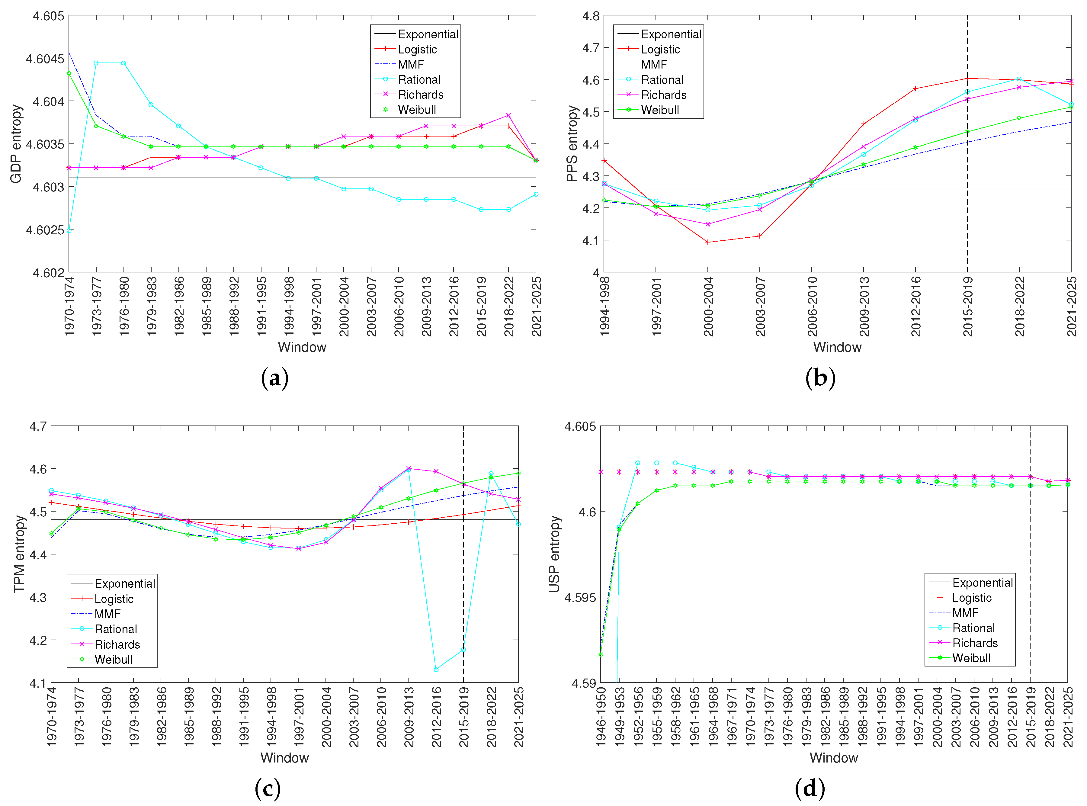
2.2. Entropy Analysis

We consider here that each data-series {GDP, PPS, TPM, USP} can be modeled as a random variable, $Y=g\left(X\right)$, where $g(·)$ represents a function given by Equations (1)–(6) and X is a random variable with probability density function (pdf) $f_x\left(x\right)$. This means that Y results from the transformation of the variable X by means of $g(·)$. The pdf of Y, $f_y\left(y\right)$, is determined by $g(·)$ and $f_x\left(x\right)$, by means of the so-called transformation technique, as follows [44].

Suppose that X is a continuous random variable with pdf $f_x(·)$, and $\mathcal{X}=\{x:f_x\left(x\right)>0\}$ denotes the set of all possible values of $f_x\left(x\right)$. Assuming that (i) function $y=g\left(x\right)$ defines a one-to-one transformation of $\mathcal{X}$ onto its domain $\mathcal{D}$, and that (ii) the derivative of $x=g^{-1}\left(y\right)$ is continuous and nonzero for $y\in \mathcal{D}$, where $g^{-1}\left(y\right)$ is the inverse function of $g\left(x\right)$, i.e., $g^{-1}\left(y\right)$ is that x for which $g\left(x\right)=y$, then $Y=g\left(X\right)$ is a continuous random variable with pdf:

$$f_y\left(y\right)=\left\{\begin{array}{c}\left|\frac{d}{dy}{g}^{-1}\left(y\right)\right|·f_x\left[g^{-1}\left(y\right)\right],\mathrm{if}y\in \mathcal{D}\hfill \\ 0,\mathrm{otherwise}\hfill \end{array}\right.$$

(7)

Once determined $f_y\left(y\right)$ we can then calculate the corresponding entropy. This scheme avoids problems that occur if we determine entropy directly based on the original data-series, since the reduced number of points available yield inaccurate histograms for estimating the pdf of the indices {GDP, PPS, TPM, USP}.

We generate a total of 10,000 points for each data-series by means of Models (1)–(6). We then adopt a sliding time window in order to slice {GDP, PPS, TPM, USP} into partially overlapping time intervals. For each window we obtain $f_y\left(y\right)$ by means of the histograms of relative frequencies with bin size $L=100$ and for a uniform pdf $f_x\left(x\right)$, where x stands for time. We then calculate the resulting Shannon entropy, S, defined by [45,46,47,48]:

$$S=-\sum _{k=1}^L{p}_{k}ln{p}_k.$$

(8)

We adopt a window length $\mathcal{W}=5$ years with $40\%$ overlap (i.e., 2 years) making a total of {18, 10, 18, 26} windows for the data-series {GDP, PPS, TPM, USP}, respectively. Alternative values for $\mathcal{W}$ were tested, but that revealed as a good compromise instantaneous and average behavior of the entropy evolution.

Figure 4 depicts the results obtained for the Exp, Log, MMF, Rat, Ric and Wei models. In general we verify a smooth variation of $S\left(t\right)$ for most cases, with exception of the Rat for the {GDP, TPM, USP}, and the MMF and Wei for the {GDP, USP}. So, the “static” methods of Subsection 2.1 and Subsection 2.2 reveal some limitations in evaluating the prediction performance of the candidate laws. In the next Section we discuss the results in the light of the dynamic behavior of these models.

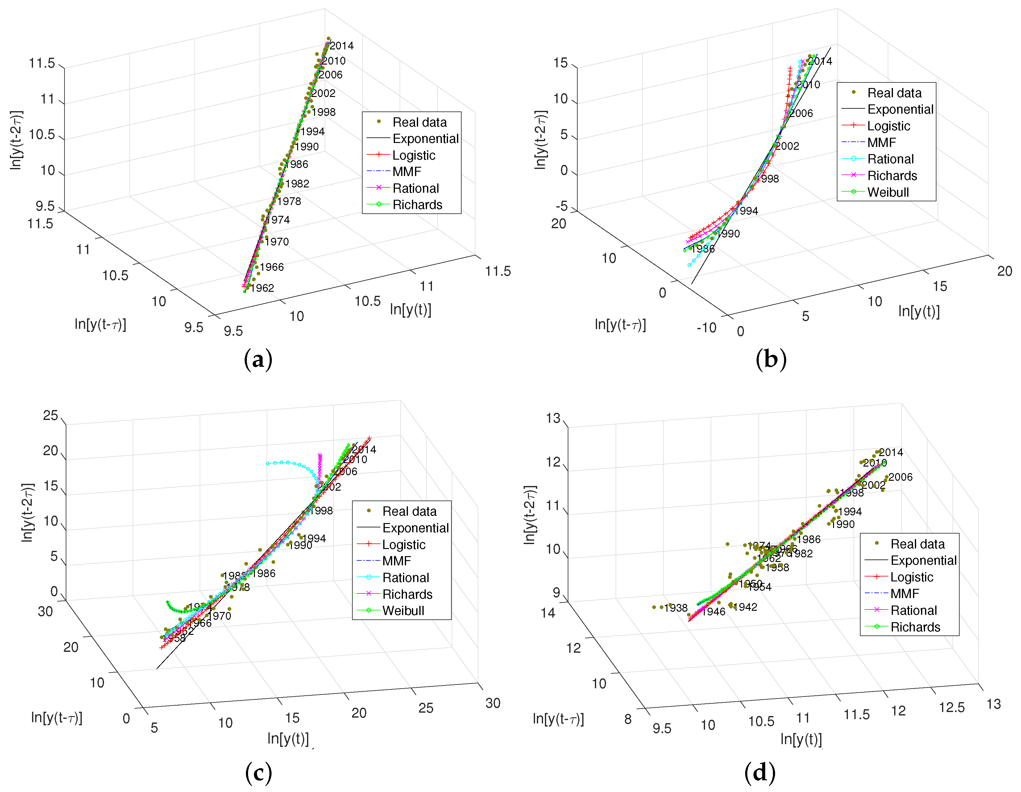
2.3. Pseudo-State Space

The PSS is a technique adopted in the context of non-linear dynamics, especially useful when there is a lack of knowledge about the system [49,50]. Generally speaking, the PSS allows a dynamical system to be represented in a higher dimensional space by taking a small sample of signals representing measurements of the system time history. The PSS is justified by Takens’ embedding theorem [51], which states that if a time series is one component of an attractor that can be represented by a smooth d-dimensional manifold. Then, the topological properties of the signal are equivalent to those of the embedding formed by the n-dimensional state space vectors:

$$\mathbf{u}\left(t\right)=\left[s\right(t),s(t-\tau ),s(t-2\tau ),\cdots ,s(t-(n-1)\tau \left)\right],$$

(9)

where $n>2d+1$, $\{d,n\}\in \mathbb{N}$ and $\tau \in {\mathbb{R}}^{+}$. Parameters τ and n denote the time delay and embedding dimension, respectively. The vector $\mathbf{u}\left(t\right)$ is commonly plotted in a n-dimensional graph, forming a trajectory. Usually we choose $n=3$, or $n=2$, in order to facilitate the interpretation of the graphs. The PSS produced by $\mathbf{u}\left(t\right)$ is expected to allow conclusions about the system dynamics [50].

A key issue in the PSS technique is the choice of τ. Intuitively, choosing τ too small will result in time series $s\left(t\right)$ and $s(t-\tau )$ close to each other, not providing two independent coordinates. On the other hand, choosing τ too large will lead to series $s\left(t\right)$ and $s(t-\tau )$ almost independent of each other, providing totally unrelated directions. Most criteria for choosing τ are based on the behavior of the autocorrelation, or the mutual information (MI), functions. The MI has the advantage of dealing well with nonlinear relations. Therefore, one possible criterion is to consider the value of τ corresponding to the first local minimum of the MI function.

The MI is a measure of how much information can be predicted about one time series, giving full information about the other [47,52]. Let X and Y represent two discrete random variables with alphabet $\mathcal{X}$ and $\mathcal{Y}$, respectively, then their mutual information $I(X,Y)$ is given by:

$$I(X,Y)=\sum _{y\in \mathcal{Y}}\sum _{x\in \mathcal{X}}p(x,y)·ln\left(\frac{p(x,y)}{p\left(x\right)·p\left(y\right)}\right),$$

(10)

where, $p\left(x\right)$ and $p\left(y\right)$ represent the marginal pdf of X and Y, respectively, and $p(x,y)$ denotes the joint pdf.

Given the real data representative of the indices {GDP, PPS, TPM, USP}, we start by calculating the MI between each data-series and their delayed versions, obtaining the minima for $\tau =\{4,4,6,4\}$ (years). In a second step, we use the Models (1)–(6) to generate year-spaced data points within the time span of the original data-series, as well as points for $2\tau$ years before and $2\tau$ after that period. These extrapolated points are then used for regenerating the data that is lost when we construct the PSS vectors in the 3-dimensional space. Therefore, each year regenerated is given by the median of the corresponding points extrapolated by the models.

Figure 5 depicts the PSS paths in log scales for $n=3$ and the indices {GDP, PPS, TPM, USP}. For the indices PPS and USP we do not include the Rat model, since it degenerates when extrapolating for certain years.

3. Discussion of the Results and Conclusions

Applied sciences are fertile in providing data that can be fitted by means of trendlines. In many cases we obtain heuristic “laws”, being particularly popular the trendlines of the exponential and power-law types [53,54,55,56,57,58,59]. The extrapolation of some “law” towards the future, as in the cases of R. Kurzweil [15] or E. Brynjolfsson [60], is often received with some skepticism by the scientific community, since future seems unpredictable a priori within present day paradigm of cause and effect. Nonetheless, the debate of predictability is out of the scope of the present paper that intends mainly to explore possible visions of the future complexity based on today’s available data.

We observe that the proposed trendlines fit well the data within the time period of the data-series. In fact, other expressions could be included in the set under analysis, that is kept to 6 just for the sake of parsimony. Therefore, the purpose of our study is to explore the behavior of such “laws” in the future and to design a scheme based on entropy to access such evolution.

Bearing these ideas in mind, adopting a time varying window and an entropy measure to evaluate the evolution of the trendline $g(·)$ can be interpreted in a probabilistic way. Time consists of an input random variable X that excites function $g\left(X\right)$ by means of a uniform pdf. Finally, the entropy measures the output random variable Y. Therefore, the real-world data-series can be interpreted as “noisy” measurements of the unknown trendline “law”.

In the present case with 4 data-series and 6 trendlines, we observe that the simple Exp function can be interpreted as a reasonable good, but not flexible, expression. In the TPM data-series the Rat function is clearly not adequate for future extrapolations, but seems to remain a valid option in the rest of the series. In what concerns the other trendlines, both the time and the entropy analysis do not lead to the emergence of one “best option”.

The 3D PSS inspired in dynamical systems seems more interesting to assess the performance of a given trendline than the 2D entropy-based approach. It is straightforward to point the Rat, Ric and Wei models for the TPM series as not adequate. Yet, in most cases we do not have an assertive criteria to decide for the “best” trendline. May be as pointed by the Danish philosopher Søren Kierkegaard “Life can only be understood backwards; but it must be lived forwards”.

References

1. Moore, G. Cramming More Components Onto Integrated Circuits. Electronics 1965, 38, 114–117. [Google Scholar] [CrossRef]
2. Tuomi, I. The lives and death of Moore’s Law. First Monday 2002, 7, 11. [Google Scholar] [CrossRef]
3. Mollick, E. Establishing Moore’s law. Ann. Histor. Comput. IEEE 2006, 28, 62–75. [Google Scholar] [CrossRef]
4. Bondyopadhyay, P.K. Moore’s law governs the silicon revolution. Proc. IEEE 1998, 86, 78–81. [Google Scholar] [CrossRef]
5. Schaller, R.R. Moore’s law: Past, present and future. Spectr. IEEE 1997, 34, 52–59. [Google Scholar] [CrossRef]
6. Moore, G. Progress in digital integrated electronics. In Proceedings of the International Electron Devices Meeting, Washington, DC, USA, 1–3 December 1975; Volume 21, pp. 11–13.
7. Sanders, T. The Moore’s Law of Moore’s Laws. MRS Bull. 2015, 40, 991–992. [Google Scholar] [CrossRef]
8. Zhang, L.; Powell, J.J.; Baker, D.P. Exponential Growth and the Shifting Global Center of Gravity of Science Production, 1900–2011. Chang. Mag. High. Learn. 2015, 47, 46–49. [Google Scholar] [CrossRef]
9. Bornmann, L.; Mutz, R. Growth rates of modern science: A bibliometric analysis based on the number of publications and cited references. J. Assoc. Inf. Sci. Technol. 2015, 66, 2215–2222. [Google Scholar] [CrossRef]
10. Korotayev, A. A compact macromodel of world system evolution. J. World Syst. Res. 2015, 11, 79–93. [Google Scholar] [CrossRef]
11. Lambert, D.R.; Joyce, M.L.; Krentler, K.A. The Multiplying Literature: Moore’s Law at Work in Marketing. In Assessing the Different Roles of Marketing Theory and Practice in the Jaws of Economic Uncertainty; Springer: Heidelberg/Berlin, Germany, 2015; pp. 114–120. [Google Scholar]
12. Chien, A.A.; Karamcheti, V. Moore’s Law: The first ending and a new beginning. Computer 2013, 48–53. [Google Scholar] [CrossRef]
13. Iyer-Biswas, S.; Crooks, G.E.; Scherer, N.F.; Dinner, A.R. Universality in stochastic exponential growth. Phys. Rev. Lett. 2014, 113, 028101. [Google Scholar] [CrossRef] [PubMed]
14. Lee, Y.; Amaral, L.A.N.; Canning, D.; Meyer, M.; Stanley, H.E. Universal features in the growth dynamics of complex organizations. Phys. Rev. Lett. 1998, 81, 3275. [Google Scholar] [CrossRef]
15. Kurzweil, R. The Law of Accelerating Returns; Springer: Heidelberg/Berlin, Germany, 2004. [Google Scholar]
16. Kim, N.S.; Austin, T.; Baauw, D.; Mudge, T.; Flautner, K.; Hu, J.S.; Irwin, M.J.; Kandemir, M.; Narayanan, V. Leakage current: Moore’s law meets static power. Computer 2003, 36, 68–75. [Google Scholar]
17. Kurzweil, R. The Singularity Is Near: When Humans Transcend Biology; Viking: New York, NY, USA, 2005. [Google Scholar]
18. Troyer, M. Beyond Moore’s law: Towards competitive quantum devices. In Proceedings of the 46th Annual Meeting of the APS Division of Atomic, Molecular and Optical Physics, Columbus, OH, USA, 8–12 June 2015; Volume 1, p. 2003.
19. Toumey, C. Less is Moore. Nat. Nanotechnol. 2016, 11, 2–3. [Google Scholar] [CrossRef] [PubMed]
20. Cavin, R.K.; Lugli, P., III; Zhirnov, V.V. Science and engineering beyond Moore’s law. Proc. IEEE 2012, 100, 1720–1749. [Google Scholar] [CrossRef]
21. Sheu, B.; Wilcox, K.; Keshavarzi, A.; Antoniadis, D. EP1: Moore’s law challenges below 10 nm: Technology, design and economic implications. In Proceedings of the 2015 IEEE International Solid-State Circuits Conference (ISSCC), San Francisco, CA, USA, 22–26 February 2015.
22. Varghese, S.; Elemans, J.A.; Rowan, A.E.; Nolte, R.J. Molecular computing: Paths to chemical Turing machines. Chem. Sci. 2015, 6, 6050–6058. [Google Scholar] [CrossRef] [Green Version]
23. Kendon, V.; Sebald, A.; Stepney, S. Heterotic computing: Exploiting hybrid computational devices. Phil. Trans. R. Soc. A 2015, 373, 20150091. [Google Scholar] [CrossRef] [PubMed]
24. Nagy, B.; Farmer, J.D.; Bui, Q.M.; Trancik, J.E. Statistical basis for predicting technological progress. PLoS ONE 2013, 8, e52669. [Google Scholar] [CrossRef] [PubMed] [Green Version]
25. Koh, H.; Magee, C.L. A functional approach for studying technological progress: Application to information technology. Technol. Forecast. Soc. Chang. 2006, 73, 1061–1083. [Google Scholar] [CrossRef]
26. Koh, H.; Magee, C.L. A functional approach for studying technological progress: Extension to energy technology. Technol. Forecast. Soc. Chang. 2008, 75, 735–758. [Google Scholar] [CrossRef]
27. Machado, J.A.T. Complex dynamics of financial indices. Nonlinear Dyn. 2013, 74, 287–296. [Google Scholar] [CrossRef]
28. Machado, J.A.T.; Mata, M.E. Pseudo phase plane and fractional calculus modeling of western global economic downturn. Commun. Nonlinear Sci. Numer. Simul. 2015, 22, 396–406. [Google Scholar] [CrossRef]
29. The World Bank. Available online: www.worldbank.org (accessed on 1 June 2016).
30. TOP500 Supercomputing Sites. Available online: http://www.top500.org/ (accessed on 1 June 2016).
31. Transistor Count. Available online: https://en.wikipedia.org/wiki/Transistor_count (accessed on 1 June 2016).
32. United States Patent and Trademark Office. Available online: http://www.uspto.gov/ (accessed on 1 June 2016).
33. Coelho, M.C.; Mendes, E.M.; Aguirre, L.A. Testing for intracycle determinism in pseudoperiodic time series. Chaos Interdiscip. J. Nonlinear Sci. 2008, 18, 023125. [Google Scholar] [CrossRef] [PubMed]
34. Kaplan, D.T.; Glass, L. Direct test for determinism in a time series. Phys. Rev. Lett. 1992, 68. [Google Scholar] [CrossRef] [PubMed]
35. Theiler, J.; Eubank, S.; Longtin, A.; Galdrikian, B.; Farmer, J.D. Testing for nonlinearity in time series: the method of surrogate data. Phys. D Nonlinear Phenom. 1992, 58, 77–94. [Google Scholar] [CrossRef]
36. Lütkepohl, H.; Xu, F. The role of the log transformation in forecasting economic variables. Empir. Econ. 2012, 42, 619–638. [Google Scholar] [CrossRef] [Green Version]
37. Fuller, S.H.; Millett, L.I. Computing performance: Game over or next level? Computer 2011, 44, 31–38. [Google Scholar] [CrossRef]
38. Hubbert, M.K. Exponential growth as a transient phenomenon in human history. In Valuing the Earth: Economics, Ecology Ethics, 2nd ed.; Daly, H.E., Townsend, K.N., Eds.; MIT Press: Cambridge, MA, USA, 1993; pp. 113–126. [Google Scholar]
39. Lopes, A.M.; Machado, J.A.T.; Pinto, C.M.; Galhano, A.M. Fractional dynamics and MDS visualization of earthquake phenomena. Comput. Math. Appl. 2013, 66, 647–658. [Google Scholar] [CrossRef]
40. Carrillo, M.; González, J.M. A new approach to modelling sigmoidal curves. Technol. Forecas. Soc. Chang. 2002, 69, 233–241. [Google Scholar] [CrossRef]
41. Tsoularis, A.; Wallace, J. Analysis of logistic growth models. Math. Biosci. 2002, 179, 21–55. [Google Scholar] [CrossRef]
42. Lawson, C.L.; Hanson, R.J. Solving Least Squares Problems; Society for Industrial and Applied Mathematics: Philadelphia, PA, USA, 1974; Volume 161. [Google Scholar]
43. Draper, N.R.; Smith, H. Applied Regression Analysis; Wiley: New York, NY, USA, 1998; Volume 3. [Google Scholar]
44. Mood, A.M.; Graybill, F.; Boes, D.C. Introduction to the Theory of Statistics; Mcgraw-Hill College: New York, NY, USA, 1974. [Google Scholar]
45. Balasis, G.; Daglis, I.A.; Papadimitriou, C.; Anastasiadis, A.; Sandberg, I.; Eftaxias, K. Quantifying dynamical complexity of magnetic storms and solar flares via nonextensive Tsallis entropy. Entropy 2011, 13, 1865–1881. [Google Scholar] [CrossRef]
46. Seely, A.J.; Newman, K.D.; Herry, C.L. Fractal Structure and Entropy Production within the Central Nervous System. Entropy 2014, 16, 4497–4520. [Google Scholar] [CrossRef]
47. Machado, J.A.T.; Lopes, A.M. Analysis and visualization of seismic data using mutual information. Entropy 2013, 15, 3892–3909. [Google Scholar] [CrossRef]
48. Machado, J.A.T.; Lopes, A.M. The persistence of memory. Nonlinear Dyn. 2014, 79, 63–82. [Google Scholar] [CrossRef]
49. Machado, J.A.T. Accessing complexity from genome information. Commun. Nonlinear Sci. Numer. Simul. 2012, 17, 2237–2243. [Google Scholar] [CrossRef]
50. Lopes, A.M.; Machado, J.A.T. Dynamic analysis of earthquake phenomena by means of pseudo phase plane. Nonlinear Dyn. 2013, 74, 1191–1202. [Google Scholar] [CrossRef]
51. Takens, F. Detecting Strange Attractors in Turbulence; Springer: Heidelberg/Berlin, Germany, 1981. [Google Scholar]
52. Shannon, C.E. A mathematical theory of communication. ACM SIGMOBILE Mob. Comput. Commun. Rev. 2001, 5, 3–55. [Google Scholar] [CrossRef]
53. Louhichi, S.; Ycart, B. Exponential growth of bifurcating processes with ancestral dependence. Adv. Appl. Probab. 2015, 47, 545–564. [Google Scholar] [CrossRef]
54. Hunt, A.G. Exponential growth in Ebola outbreak since May 14, 2014. Complexity 2014, 20, 8–11. [Google Scholar] [CrossRef]
55. Serbyn, M.; Papić, Z.; Abanin, D.A. Universal slow growth of entanglement in interacting strongly disordered systems. Phys. Rev. Lett. 2013, 110, 260601. [Google Scholar] [CrossRef] [PubMed]
56. Rodriguez-Brenes, I.A.; Komarova, N.L.; Wodarz, D. Tumor growth dynamics: Insights into evolutionary processes. Trends Ecol. Evol. 2013, 28, 597–604. [Google Scholar] [CrossRef] [PubMed]
57. Pinto, C.; Mendes Lopes, A.M.; Machado, J.A.T. A review of power laws in real life phenomena. Commun. Nonlinear Sci. Numer. Simul. 2012, 17, 3558–3578. [Google Scholar] [CrossRef]
58. Clauset, A.; Shalizi, C.R.; Newman, M.E. Power-law distributions in empirical data. SIAM Rev. 2009, 51, 661–703. [Google Scholar] [CrossRef]
59. Quine, M.; Robinson, J. A linear random growth model. J. Appl. Probab. 1990, 27, 499–509. [Google Scholar] [CrossRef]
60. Brynjolfsson, E.; McAfee, A. The Second Machine Age: Work, Progress, and Prosperity in a Time of Brilliant Technologies; W. W. Norton & Company: New York, NY, USA, 2014. [Google Scholar]
Figure 1. Correlogram for the data-series y ˜ i : (a) GDP; (b) PPS; (c) TPM; (d) USP.
Entropy 18 00217 g001
Figure 2. Time evolution of the logarithm of the data-series, y ˜ i , and the model approximations, y ^ i : (a) GDP; (b) PPS; (c) TPM; (d) USP.
Entropy 18 00217 g002aEntropy 18 00217 g002b
Figure 3. Residuals ( y ˜ i - y ^ i ) 2 of the fits generated by nonlinear least-squares: (a) GDP; (b) PPS; (c) TPM; (d) USP.
Entropy 18 00217 g003aEntropy 18 00217 g003b
Figure 4. Entropy per window for the 6 model approximations: (a) GDP; (b) PPS; (c) TPM; (d) USP.
Entropy 18 00217 g004
Figure 5. Real and model approximated PSS plots (in log units): (a) GDP; (b) PPS; (c) TPM; (d) USP.
Entropy 18 00217 g005