Single Neuron Stochastic Predictive PID Control Algorithm for Nonlinear and Non-Gaussian Systems Using the Survival Information Potential Criterion

Abstract

This paper presents a novel stochastic predictive tracking control strategy for nonlinear and non-Gaussian stochastic systems based on the single neuron controller structure in the framework of information theory. Firstly, in order to characterize the randomness of the control system, survival information potential (SIP), instead of entropy, is adopted to formulate the performance index, which is not shift-invariant, i.e., its value varies with the change of the distribution location. Then, the optimal weights of the single neuron controller can be obtained by minimizing the presented SIP based predictive control criterion. Furthermore, mean-square convergence of the proposed control algorithm is also analyzed from the energy conservation perspective. Finally, a numerical example is given to show the effectiveness of the proposed method.

1. Introduction

Since almost all the control systems are subject to random signals (such as those originating from system parameter variations and sensor noise, etc.), stochastic systems are widely encountered in control engineering design. Minimizing the randomness in the closed-loop system is one of the important practical issues in controller design. Therefore, minimum variance control [1] has been obtained significant attentions. Its purpose is to minimize variations in the controlled system outputs or the tracking errors. Indeed, even today, most stochastic control design methods have only focused on control of the output mean and the variance of stochastic systems. In general, these developments are done mostly based on the assumptions that the system variables are of Gaussian types. Such assumptions, although strict, allow control engineers to make use of the well-established stochastic theory to perform controller design and closed-loop system analysis.

In industrial processes, product quality data can be approximated by the Gaussian probability density function (PDF) when the system operates normally. However, when abnormality occurs along the production line, the variabilities of these quality variables would not follow Gaussian distributions. In this regard, actions need to be taken so that the manipulated variables can be tuned to bring these quality variables back to certain desired ones. In fact, most industrial processes have difficulty meeting the Gaussian assumption because of the mixture of different courses with Gaussian disturbances or other factors. Moreover, the nonlinearity in stochastic systems could lead to non-Gaussian randomness even if the disturbances follow a Gaussian distribution. Thus, controlling the mean and variance of system variables may be far from sufficiently characterizing the statistical property of the stochastic processes. It is known that, in many cases, the behavior of a stochastic process can be completely characterized by the shape of its statistical distribution represented by PDF. Therefore, for analysis and design purposes, it is important to consider the entire PDF. PDF-shaping control design accounts for the issues mentioned above by selecting a certain shape for the process PDF as the goal of the control design procedure would provide an accurate and flexible control strategy that can accommodate a wide class of objectives.

In order to solve the problems existing in paper-making processes, the stochastic distribution control (SDC) theory was proposed by Wang (1996) [2]. This theory aims at controlling the shape of the output PDF instead of the mean and variance for stochastic systems [3,4,5]. After that, SDC has been used to handle the stochastic systems with non-Gaussian disturbances. Then, a linear-matrix-inequality- based convex optimization algorithm was developed for control, filter design and fault detection in non-Gaussian systems [6,7,8]. Nevertheless, the PDFs of the output are not necessarily measurable; instead, a more general measure of uncertainty, namely the entropy, has been used to characterize the uncertainty of the output tracking error. Compared with SDC (PDF shaping strategy) proposed earlier, it is more straightforward to us a minimum error entropy (MEE) based stochastic control algorithm to design a controller for tracking errors. It is more appropriate than the traditional minimum mean square error (MSE) criterion when dealing with nonlinearities and non-Gaussian disturbances. Shannon entropy is the most important and commonly used method in MEE based stochastic control [9,10,11]. A well-known generalization of Shannon entropy is Renyi entropy. When the order of Renyi entropy approaches 1, Renyi entropy will reduce and become Shannon entropy. The argument of the log in Renyi entropy is named the information potential (IP) and used as an alternative entropy criterion because of its monotonic property. Puya et al. [12] applied the minimum Renyi entropy control scheme to decrease the closed-loop randomness of the output under an iterative learning control (ILC) basis for general nonlinear and unknown non-Gaussian stochastic systems. Besides, information potential (IP) based dynamic neural networks were used to perform the modeling and control of the plant. In [13], the quadratic IP of tracking errors was employed to design controllers for nonlinear multivariate and non-Gaussian systems. $(h,\varphi )\mathrm{-entropy}$ is the most generalized definition of entropy [14]. $(h,\varphi )\mathrm{-entropy}$ has been employed in stochastic control systems [15,16]. Ren et al. [15] proposed a new tracking control algorithm for a class of networked control systems (NCSs) with non-Gaussian random disturbances and delays. Zhang et al. [16] presented an improved single neuron controller for multivariable stochastic systems with non-Gaussianities and unmodeled dynamics by minimizing $(h,\varphi )\mathrm{-entropy}$ of tracking errors.

The Shannon and order-$\alpha$ Renyi entropies of a continuous random variable are both defined based on the probability density function. This kind of entropy has several drawbacks. (1) The definition will be ill-suited for the case in which PDF does not exist; (2) the value can be negative; (3) the approximation using empirical distribution is impossible in general. And the IP criterion is conservative. It should be maximized to achieve smaller errors only when $\alpha >1$. Some new definitions of entropy have been made to solve these problems. Rao et al. [17] proposed the cumulative residual entropy (CRE), which is defined based on the cumulative distribution function. In [18], Zografos and Nadarajah proposed the survival exponential and the generalized survival exponential entropies, both of which are broad entropy definitions based on the survival function and include CRE as a special case.

In this paper, survival information potential (SIP), proposed by Chen et al. [19], will be utilized to construct the performance index of stochastic control systems. Compared with the MEE criterion, adding a bias term to the tracking error [6,9,10,13] would not be necessary because of the shift-variance property of the SIP. In the previous work of MEE control [9,10,11,12,13,14,15,16], although the randomness of control input exists in practical conditions, the control input was considered as a deterministic variable for simplicity, which is unsuitable and conservative. Therefore, in this paper, the performance index with the integration of SIPs of the control input and the tracking error is proposed.

The predictive control idea was brought up as an industrial approach to process control in the 1970s. Today this technique is the most frequently applied advanced process control method in the industry. The stochastic distribution control algorithms have been extended by the advanced control algorithm to increase the control performance. So far mainly two classes of algorithms have been developed for systems affected by stochastic noise and subject to probabilistic state and/or input constraints. (1) The randomized, or scenario-based approach [20,21,22]: It is a very general methodology that can consider linear or nonlinear systems affected by noise with general distributions characterized by possibly unbounded and nonconvex support. (2) The probabilistic approximation approach [23,24,25,26,27,28]: It is based on the point-wise reformulation of probabilistic or expectation constraints in deterministic terms to be included in the MPC formulation. Reference [29] gave an overview of the main developments in the area of stochastic model predictive control (SMPC) in the past decade. It described different SMPC algorithms and the key theoretical challenges in stochastic predictive control without undue mathematical complexity. However, the above results were obtained under the assumption that the system variables obey Gaussian distribution, and only mean value and variance were considered. As presented above, PDF contains the whole characteristics of random variables. From this perspective, SMPC approaches to a class of nonlinear systems with unbounded stochastic uncertainties were proposed in [30,31]. In [30], the Fokker–Planck equation was used for describing the dynamic evolution of the states’ PDFs and the closed-loop stability was ensured by designing a stability constraint in terms of a stochastic control Lyapunov function. Polynomial chaos expansions were utilized to propagate the probabilistic parametric uncertainties through the system model in [31]. In the framework of SDC, SMPC was used to control the molecular weight distribution (MWD) [32,33] with the existence of non-Gaussian noises. As mentioned previously, considering the non-Gaussian SMPC in the statistical information framework may be an alternative and effective method.

Based on the preliminary work [19,34,35,36,37], in this paper, a single neuron stochastic predictive control method for nonlinear stochastic discrete systems affected by non-Gaussian noise is proposed. The proposed algorithm will be detailed in the rest of the sections. In Section 2, the models of the nonlinear stochastic system and single neuron controller are firstly presented. Then a new SIP-based predictive criterion, which contains both the randomness of tracking errors and the control input, is formulated. Based on the established models and the new criterion, the single neuron stochastic predictive control (SNSPC) algorithm is derived and the online computation procedure is also summarized. To analyze the convergence of the proposed control algorithm, the energy conversion principle is used in Section 3. A numerical simulation example is introduced to illustrate the efficiency of the proposed control strategy in Section 4. The last section concludes this paper.

2. Single Neuron Stochastic Predictive Control (SNSPC)

2.1. System Model and Single Neuron Controller

A general discrete, nonlinear dynamic system with process disturbances and measurement noises is considered here. It is described in the state-space form as:

$$\{\begin{array}{l}{x}_{k+1}=f\left(x_k,u_k,{\zeta }_k\right)\\ y_k=g\left(x_k,u_k,{\nu }_k\right)\end{array}$$

(1)

where $x_k\in {ℝ}^n$ is the state, $y_k\in ℝ$ is the measured output, and $u_k\in ℝ$ is the control input. ${\zeta }_k$ and ${\nu }_k$ are external disturbances in the input and the measurement channels, respectively and they may not follow Gaussian distributions. $f(\cdot )$ and $g(\cdot )$ are known nonlinear functions that represent the system dynamics.

The goal of the control design is to find the optimal control input to make the output track the desired set-point $r_k$ as soon as possible. Due to the nonlinearity and disturbances involved in the system (1), the traditional PID control algorithm cannot have excellent performance here. In the past work, a single neuron adaptive PID controller has the advantages of neural network intelligent control and PID control. Single neuron adaptive PID controller achieves control system’s self-organization, adaptive function by adjusting weighting coefficients with the changes of the control parameters [35]. The controller is a multiple input and single output nonlinear processing unit with self-learning ability. The output of the single neuron adaptive PID controller is shown as Equation (2):

$$u_k=u_{k-1}+K{\displaystyle \sum _{l=1}^3{w}_{lk}{x}_{lk}}/\Vert {\Sigma }_k\Vert$$

(2)

where ${\Sigma }_k={\displaystyle \sum _{l=1}^3{w}_{lk}}$, $K>0$ is the proportional coefficient of the neuron. $w_{lk}$ $(l=1,2,3)$ stands for the weight corresponding to each input. $x_{lk}(l=1,2,3)$ is the input of the neuron from the tracking error $e_k$ and it can be defined as:

$$\{\begin{array}{l}{x}_{1k}=e_k\\ x_{2k}=e_k-e_{k-1}\\ x_{3k}=e_k-2e_{k-1}+e_{k-2}\end{array}$$

(3)

Remark 1. $x_{lk}(l=1,2,3)$ is the input of the neuron from the tracking error $e_k$. The weights $x_{lk}(l=1,2,3)$ reflect the dynamic characteristics of the controlled object and the process response. The neuron weights can be updated through self-learning strategy, and the tracking error can be correspondingly eliminated and approach to the steady state effected by three kinds of control parts together.

2.2. SIP-Based Predictive Criterion

If noises ${\zeta }_k$ and ${\nu }_k$ are not Gaussian, the variance of the output tracking error $e_k=r_k-y_k$ would not be sufficient to characterize the randomness of the tracking error dynamic systems. Therefore, an alternative measure of uncertainty, survival information potential (SIP), is given to construct the performance index for measuring the dispersion of the stochastic systems.

Firstly, the definition and properties of SIP are presented as follows.

Definition 1. 

Definition of SIP [19]: For a random vector $X$ in ${ℝ}^m$, SIP of order $\alpha (\alpha >0)$ is defined by

$$S_{\alpha }\left(X\right)={\displaystyle {\int }_{{ℝ}_{+}^m}{\overline{F}}_{\left|X\right|}^{\alpha }\left(x\right)dx}$$

(4)

where ${\overline{F}}_{\left|X\right|}\left(x\right)=P\left(\left|X\right|>x\right)=E\left[I\left(\left|X\right|>x\right)\right]$ is the multivariate survival function (or equivalently, the distribution function) of the random vector $\left|X\right|$, and ${ℝ}_{+}^m=\{x\in {ℝ}^m:x=\left(x_1,\cdots ,x_m\right),x_i\ge 0,i=1,\cdots ,m\}$. Note that $\left|X\right|>x$ means $\left|X_i\right|>x_i,i=1,\dots ,m$ and $I(\cdot )$ is the indicator function. Similarly, when $\alpha =2$, SIP is called the quadratic survival information potential (QSIP).

Property 1. 

Property 1 of SIP [19]: $S_{\alpha }\left(X\right)\ge 0$, with equality if and only if $P\left(X=0\right)=1$.

Property 2. 

Property 2 of SIP [19]: Let $X$ be an m-dimensional random vector, and let another m-dimensional random vector $Y={(Y_1,Y_2,\cdots Y_m)}^{\mathrm{T}}$ with $Y_i=c_i{X}_i$, $c_i\in ℝ$, $i=1,2,\cdots m$, then $S_{\alpha }\left(Y\right)=\left({\displaystyle {\prod }_{i=1}^m\left|c_i\right|}\right)S_{\alpha }\left(X\right)$.

Remark 2. 

SIP has some advantages over the IP: (1) It has consistent definition in the continuous and discrete domains; (2) it is not shift-invariant (i.e., its value would vary with the location of distribution); (3) it can be computed more easily from the sample data (without kernel computation and the choice of the kernel width), and the estimation asymptotically converges to the true value; (4) it is a more robust measure since the distribution function is more regular than the density function. (Note that the density is computed as the derivative of the distribution.)

Because of the nonlinearity and noises involved in the system, the tracking error is a non-Gaussian stochastic variable at a typical instant. Therefore, the control input is also non-Gaussian according to the single neuron controller Equations (2) and (3). However, in the previous work on stochastic distribution control [9,10,11,12,13,15,16], the control input is considered as a deterministic variable, which is conservative. And moreover, the multi-step predictive control strategy which can achieve better performance in industrial processes is adopted to design the optimal control input here.

The cost function of a SIP-based predictive controller for set point control is similar to that of a conventional predictive control with a continuous actor, but the SIP criterion is used in the control design instead of the MSE criterion

$$J={\displaystyle \sum _{i=1}^P{S}_{\alpha }\left(e_{k+i-1}\right)}+\lambda {\displaystyle \sum _{j=1}^M{S}_{\alpha }\left(u_{k+j-1}\right)}$$

(5)

where $e_{k+i}$ is the i-step ahead prediction of the system tracking error. $P$ and $M$ are the prediction horizon and the control horizon, respectively, and $M\le P$. It is assumed that the control variable would not change after $M$ steps, i.e., $u_{k+j-1}=u_{k+M-1}(j>M)$.

2.3. SNSPC Algorithm

Based on the structure of the single neuron adaptive controller Equations (2) and (3) and the performance index Equation (5), the optimal weights of the single neuron can be solved by the stochastic gradient method

$$w_k^{*}=\underset{W_k\in {ℝ}^{3M}}{\arg \min } J=\underset{w_k\in {ℝ}^{3M}}{\arg \min }\left\{{\displaystyle \sum _{i=1}^P{S}_{\alpha }\left(e_{k+i-1}\right)}+\lambda {\displaystyle \sum _{j=1}^M{S}_{\alpha }\left(u_{k+j-1}\right)}\right\}$$

(6)

where $w_k={\left[w_{1k}{w}_{2k}{w}_{3k}{w}_{1,k+1}{w}_{2,k+1}{w}_{3,k+1}\cdots w_{1,k+M-1}{w}_{2,k+M-1}{w}_{3,k+M-1}\right]}^{\mathrm{T}}\in {ℝ}^{3M}$.

According to the definition of SIP, the optimal weights $w_k^{*}$ can be calculated from

$$\frac{\partial J}{\partial w_k}=\frac{\partial }{\partial w_k}\left\{{\displaystyle \sum _{i=1}^P{\displaystyle {\int }_{-\infty }^{+\infty }{\overline{F}}_{\left|e_{k+i-1}\right|}}\left(x\right)dx}+\lambda {\displaystyle \sum _{j=1}^M{\displaystyle {\int }_{-\infty }^{+\infty }{\overline{F}}_{\left|u_{k+j-1}\right|}}\left(z\right)dz}\right\}=0$$

(7)

where ${\overline{F}}_{\left|e_{k+i-1}\right|}$ and ${\overline{F}}_{\left|u_{k+j-1}\right|}$ are the survival functions of the tracking error $e_{k+i-1}$ and the control input $u_{k+j-1}$, respectively.

In the practical application, it is generally difficult to develop a comprehensive first-principle model to describe the distribution of the error $e_k$. Instead of the theoretical SIP, the data-driven empirical SIP used as the cost function would be useful alternative to timely online prediction of the errors. Given a sequence of error samples $\left(e_{1k},e_{2k},\cdots ,e_{\overline{N}k}\right)$, assuming, without the loss of generality, that $\left|e_{1k}\right|\le \left|e_{2k}\right|\le \left|e_{\overline{N}k}\right|$, the empirical SIP would be [20]

$${\widehat{S}}_{\alpha }\left(e_k\right)={\displaystyle \sum _{j=1}^{\overline{N}}{\mu }_j\left|e_{jk}\right|}$$

(8)

where ${\mu }_j={\left(\frac{\overline{N}-j+1}{\overline{N}}\right)}^{\alpha }-{\left(\frac{\overline{N}-j}{\overline{N}}\right)}^{\alpha }$.

Similarly, the empirical SIP of $u_{k+j-1}$, ${\widehat{S}}_{\alpha }\left(u_{k+j-1}\right)$, can also be formulated. The empirical cost Equation (8) is the weighted sum of the ordered absolute errors. One drawback of this empirical SIP criterion is that it is not smooth at $e_{jk}=0$ and $u_{jk}=0$. To address this problem, a more general cost can be defined using the empirical SIP of any mapped errors and inputs; that is,

$$\overline{J}\left(e_{k:k+P-1}\right)={\displaystyle \sum _{i=1}^P{\widehat{S}}_{\alpha }\left(\varphi \left(e_{k+i-1}^{}\right)\right)}+\lambda {\displaystyle \sum _{j=1}^M{\widehat{S}}_{\alpha }\left(\varphi \left(u_{k+j-1}^{}\right)\right)}={\displaystyle \sum _{i=1}^P{\displaystyle \sum _{l=1}^{\overline{N}}{\mu }_l\varphi \left(e_{l,k+i-1}\right)}}+\lambda {\displaystyle \sum _{j=1}^M{\displaystyle \sum _{l=1}^{\overline{N}}{\sigma }_l\varphi \left(u_{l,k+j-1}\right)}}$$

(9)

where $e_{k:k+P-1}={\left[\begin{array}{cccc}{e}_k& e_{k+1}& \cdots & e_{k+P-1}\end{array}\right]}^{\mathrm{T}}$, ${\mu }_l={\left(\frac{\overline{N}-l+1}{\overline{N}}\right)}^{\alpha }-{\left(\frac{\overline{N}-l}{\overline{N}}\right)}^{\alpha }$. The mapping function $\varphi (\cdot )$ usually satisfies

$$\{\begin{array}{l}(i)\mathrm{positivity}:\varphi (\cdot )\ge 0\\ (ii)\mathrm{symmetry}:\varphi \left(x\right)=\varphi \left(-x\right)\\ (iii)\mathrm{monotonicity}:\left|x_1\right|<\left|x_2\right|\Rightarrow \varphi \left(x_1\right)\le \varphi \left(x_2\right)\end{array}$$

(10)

Remark 3. As the data-driven empirical SIP-based performance index is not smooth at $e_{jk}=0$ and $u_{jk}=0$, a proper function transformation method can be used to establish an equivalent SIP-based criterion, which can be formulated as Equation (9) and (10). In the simulation, the empirical SIP of the square errors $\left(e_{1k}^2,e_{2k}^2,\cdots ,e_{\overline{N}k}^2\right)$ and the square control inputs $\left(u_{1k}^2,u_{2k}^2,\cdots ,u_{\overline{N}k}^2\right)$ as an alternative adaptation cost is used here, given by

$$\overline{J}={\displaystyle \sum _{i=1}^P{\widehat{S}}_{\alpha }\left(e_{k+i-1}^2\right)}+\lambda {\displaystyle \sum _{j=1}^M{\widehat{S}}_{\alpha }\left(u_{k+j-1}^2\right)}={\displaystyle \sum _{i=1}^P{\displaystyle \sum _{l=1}^{\overline{N}}{\mu }_l{e}_{l+i-1}^2}}+\lambda {\displaystyle \sum _{j=1}^M{\displaystyle \sum _{l=1}^{\overline{N}}{\sigma }_l{u}_{l+j-1}^2}}$$

The above cost is the weighted sum of the ordered square errors with the popular minimum mean square error (MSE) criterion as a special case (when α = 1).

Based on the general cost Equation (9), the weight update equation for adaptive system training is

$$w_{k+1}=w_k-\eta \frac{\partial \overline{J}}{\partial w_k}=w_k-\eta \frac{\partial e_{k:k+P-1}^{\mathrm{T}}}{\partial w_k}\frac{\partial \overline{J}}{\partial e_{k:k+P-1}}$$

(11)

where $\eta >0$ denotes the step-size (or adaptation gain).

According to the above presentation, the optimal input can be computed. The procedure below describes the steps of implementing SNSPC specifically.

Step 1: Initialize the weight vector of the single neuron $w_0$. Choose the α value, step-size $\eta$, and the sliding window length $\overline{N}$.

Step 2: Estimate the performance index using empirical SIPs of the output tracking error and the control input in (9).

Step 3: Solve the optimal weight vector $w_k^{*}$ by (11).

Step 4: Compute the next control input

$$u_k=u_{k-1}+\frac{K}{\Vert {\Sigma }_k\Vert }\left[\begin{array}{ccc}{x}_{1k}& x_{2k}& x_{3k}\end{array}\right]\left[\begin{array}{cc}{I}_{3\times 3}& 0_{3\times (3P-3)}\end{array}\right]w_k^{*}$$

(12)

and implement the input on the process.

Step 5: Collect the process outputs to update the SIPs of the output tracking error and the control input. Then repeat the procedure from Step 2 to Step 5 for the next time step, $k=k+1$.

Remark 4. 

The computations of the SIP-based performance index in Equation (9) are easier than the minimum error entropy (MEE) criterion, because the index is directly computed from the sample data without kernel computation and the choice of the kernel width, but the major computations of the partial derivative, $\frac{\partial e_{k:k+P-1}^{\mathrm{T}}}{\partial w_k}$, in the control algorithm Equation (12) would be done.

3. Mean-Square Stability

In order to analyze the convergence of the proposed control algorithm, the nonlinear stochastic system Equation (1) is firstly linearized as

$$\{\begin{array}{l}\Delta x_{k+1}={\frac{\partial f}{\partial x}|}_{x_{k-1}}\Delta x_k+{\frac{\partial f}{\partial u}|}_{u_{k-1}}\Delta u_k+{\frac{\partial f}{\partial \zeta }|}_{{\zeta }_{k-1}}\Delta {\zeta }_k\\ \Delta y_k={\frac{\partial g}{\partial x}|}_{x_{k-1}}\Delta x_k+{\frac{\partial g}{\partial u}|}_{u_{k-1}}\Delta u_k+{\frac{\partial g}{\partial \nu }|}_{{\nu }_{k-1}}\Delta {\nu }_k\end{array}$$

(13)

where $\Delta u_k=u_k-u_{k-1}$, $\Delta x_k=x_k-x_{k-1}={\tilde{x}}_k$, $\Delta {\zeta }_k={\zeta }_k-{\zeta }_{k-1}={\tilde{\zeta }}_k$, $\Delta y_k=y_k-y_{k-1}={\tilde{y}}_k$, and $\Delta {\nu }_k={\nu }_k-{\nu }_{k-1}={\tilde{\nu }}_k$. It can be simply denoted as

$$\{\begin{array}{l}{\tilde{x}}_{k+1}=A_k{\tilde{x}}_k+B_k\Delta u_k+N_{1k}{\tilde{\zeta }}_k\\ {\tilde{y}}_k=C_k{\tilde{x}}_k+D_k\Delta u_k+N_{2k}{\tilde{\nu }}_k\end{array}$$

(14)

where ${A_k=\frac{\partial f}{\partial x}|}_{x_{k-1}}$, ${B_k=\frac{\partial f}{\partial u}|}_{u_{k-1}}$, $C_k={\frac{\partial g}{\partial x}|}_{x_{k-1}}$, $D_k={\frac{\partial g}{\partial u}|}_{u_{k-1}}$, $N_{1k}={\frac{\partial f}{\partial \zeta }|}_{{\zeta }_{k-1}}$, $N_{2k}={\frac{\partial g}{\partial \nu }|}_{{\nu }_{k-1}}$.

Based on the state space representation, an extended state space model can be formulated as [36]

$$y_k^f=L_k^v{m}_k^p+L_k^u{u}_k^f+L_k^{\varsigma }{\varsigma }_k^f$$

(15)

where $y_k^f={\left[\begin{array}{ccc}{\tilde{y}}_k& \cdots & {\tilde{y}}_{k+M-1}\end{array}\right]}^{\mathrm{T}}$, $u_k^f={\left[\begin{array}{ccc}\Delta u_k& \cdots & \Delta u_{k+M-1}\end{array}\right]}^{\mathrm{T}}$, $m_k^p={\left[\begin{array}{cc}{\left(v_{1k}^p\right)}^{\mathrm{T}}& {\left(v_{2k}^p\right)}^{\mathrm{T}}\end{array}\right]}^{\mathrm{T}}$, $v_{1k}^p={\left[\begin{array}{ccc}{\tilde{y}}_{k-M}& \cdots & {\tilde{y}}_{k-1}\end{array}\right]}^{\mathrm{T}}$, $v_{2k}^p={\left[\begin{array}{ccc}\Delta u_{k-M}& \cdots & \Delta u_{k-1}\end{array}\right]}^{\mathrm{T}}$. $L_k^v$, $L_k^u$ and $L_k^{\varsigma }$ can be obtained from Equation (14); ${\varsigma }_k^f$ is the composite noise, including external noises (${\zeta }_k$ and ${\nu }_k$) and the model mismatch randomness, and it may be non-Gaussian noises.

From Equation (2), Equation (15) can be reformulated as

$$y_k^f=L_k^v{m}_k^p+L_k^u{\chi }_k{w}_k+L_k^{\varsigma }{\varsigma }_k^f$$

(16)

where ${\chi }_k$ is the input matrices of the single neural network, which consists of tracking errors:

$${\chi }_k=\left[\begin{array}{cccc}{z}_k& 0& 0& 0\\ z_k& z_{k+1}& 0& 0\\ ⋮& ⋮& \ddots & ⋮\\ z_k& z_{k+1}& \cdots & z_{k+M}\end{array}\right]$$

where $z_k=\left[\begin{array}{ccc}\frac{K}{\Vert {\Sigma }_k\Vert }{x}_{1k}& \frac{K}{\Vert {\Sigma }_k\Vert }{x}_{2k}& \frac{K}{\Vert {\Sigma }_k\Vert }{x}_{3k}\end{array}\right]$ and $0=\left[\begin{array}{ccc}0& 0& 0\end{array}\right]$.

Thus, the difference between the future predictions and the set-point trajectory is

$$e_k^f=L_k^v{m}_k^p+L_k^u{\chi }_k{w}_k+L_k^{\varsigma }{\varsigma }_k^f-\Delta r_k^f$$

(17)

where $\Delta r_k^f=r_k^f-r_{k-1}^f$ is the change of the set-point at time point $k$ and ${\mathsf{\theta }}_k=L_k^v{m}_k^p+L_k^{\varsigma }{\varsigma }_k^f-\Delta r_k^f$, which is a new random vector; then Equation (17) can be rewritten as

$$e_k^f=L_k^u{\chi }_k{w}_k+{\mathsf{\theta }}_k$$

(18)

Now a priori error vector and a posteriori error vector, $e_k^{af}$ and $e_k^{pf}$, are defined as:

$$\{\begin{array}{l}{e}_k^{af}=L_k^u{\chi }_k{w}_k\\ e_k^{pf}=L_k^u{\chi }_k{w}_{k+1}\end{array}$$

(19)

Obviously, $e_k^{af}$ and $e_k^{pf}$ have the following relationship

$$e_k^{pf}=e_k^{af}+L_k^u{\chi }_k\left(w_{k+1}-w_k\right)$$

(20)

By incorporating Equation (11), the following equation is gotten,

$$e_k^{pf}=e_k^{af}-L_k^u{\chi }_k\eta \frac{\partial {\left(e_k^f\right)}^{\mathrm{T}}}{\partial w_k}\frac{\partial \overline{J}}{\partial e_k^f}=e_k^{af}+\eta L_k^u{\chi }_k{\chi }_k^{\mathrm{T}}{L}_u^{\mathrm{T}}\overline{h}\left(e_k^f\right)$$

(21)

where $\overline{h}\left(e_k^f\right)=\frac{\partial \overline{J}}{\partial e_k^f}={\left[\begin{array}{cccc}\frac{\partial \overline{J}}{\partial e_k}& \frac{\partial \overline{J}}{\partial e_{k+1}}& \cdots & \frac{\partial \overline{J}}{\partial e_{k+M-1}}\end{array}\right]}^{\mathrm{T}}$. $R_k=L_k^u{\chi }_k{\left(L_k^u{\chi }_k\right)}^{\mathrm{T}}$ is an $M\times M$ -dimensional symmetric matrix. Assume $R_k$ is invertible (i.e., $\det R_k\ne 0$),

$$\begin{array}{l}{e}_k^{pf}=e_k^{af}+\eta R_k\overline{h}\left(e_k^f\right)\\ R_k^{-1}\left(e_k^{pf}-e_k^{af}\right)=\eta \overline{h}\left(e_k^f\right)\\ {\chi }_k^{\mathrm{T}}{\left(L_k^u\right)}^{\mathrm{T}}{R}_k^{-1}\left(e_k^{pf}-e_k^{af}\right)=\eta {\chi }_k^{\mathrm{T}}{\left(L_k^u\right)}^{\mathrm{T}}\overline{h}\left(e_k^f\right)\\ {\chi }_k^{\mathrm{T}}{\left(L_k^u\right)}^{\mathrm{T}}{R}_k^{-1}\left(e_k^{pf}-e_k^{af}\right)=\left(w_{k+1}-w_k\right)\end{array}$$

(22)

And hence

$$w_{k+1}=w_k+{\chi }_k^{\mathrm{T}}{\left(L_k^u\right)}^{\mathrm{T}}{R}_k^{-1}\left(e_k^{pf}-e_k^{af}\right)$$

(23)

Both sides of Equation (23) should have the same energy; that is

$$\begin{array}{l}{w}_{k+1}^{\mathrm{T}}{w}_{k+1}={\left[w_k+{\chi }_k^{\mathrm{T}}{\left(L_k^u\right)}^{\mathrm{T}}{R}_k^{-1}\left(e_k^{pf}-e_k^{af}\right)\right]}^{\mathrm{T}}\times \left[w_k+{\chi }_k^{\mathrm{T}}{\left(L_k^u\right)}^{\mathrm{T}}{R}_k^{-1}\left(e_k^{pf}-e_k^{af}\right)\right]\\ =w_k^{\mathrm{T}}{w}_k+2w_k^{\mathrm{T}}{\chi }_k^{\mathrm{T}}{\left(L_k^u\right)}^{\mathrm{T}}{R}_k^{-1}\left(e_k^{pf}-e_k^{af}\right)\\ +{\left(e_k^{pf}-e_k^{af}\right)}^{\mathrm{T}}{R}_k^{-\mathrm{T}}\left(L_k^u\right){\chi }_k{\chi }_k^{\mathrm{T}}{\left(L_k^u\right)}^{\mathrm{T}}{R}_k^{-1}\left(e_k^{pf}-e_k^{af}\right)\end{array}$$

(24)

From $R_k=L_k^u{\chi }_k{\left(L_k^u{\chi }_k\right)}^{\mathrm{T}}$, we have

$$\begin{array}{l}{w}_{k+1}^{\mathrm{T}}{w}_{k+1}=w_k^{\mathrm{T}}{w}_k+2w_k^{\mathrm{T}}{\chi }_k^{\mathrm{T}}{\left(L_k^u\right)}^{\mathrm{T}}{R}_k^{-1}\left(e_k^{pf}-e_k^{af}\right)+{\left(e_k^{pf}-e_k^{af}\right)}^{\mathrm{T}}{R}_k^{-1}\left(e_k^{pf}-e_k^{af}\right)\\ =w_k^{\mathrm{T}}{w}_k+2w_k^{\mathrm{T}}{\chi }_k^{\mathrm{T}}{\left(L_k^u\right)}^{\mathrm{T}}{R}_k^{-1}\left(e_k^{pf}-e_k^{af}\right)+{\left(e_k^{pf}\right)}^{\mathrm{T}}{R}_k^{-1}{e}_k^{pf}\\ -2{\left(e_k^{af}\right)}^{\mathrm{T}}{R}_k^{-1}{e}_k^{pf}+{\left(e_k^{af}\right)}^{\mathrm{T}}{R}_k^{-1}{e}_k^{af}\end{array}$$

(25)

Since $R_k^{-1}={\left(L_k^u\right)}^{-\mathrm{T}}{\chi }_k^{-\mathrm{T}}{\chi }_k^{-1}{\left(L_k^u\right)}^{-1}$, $e_k^{af}=L_k^u{\chi }_k{w}_k$, then

$$\begin{array}{l}{w}_{k+1}^{\mathrm{T}}{w}_{k+1}=w_k^{\mathrm{T}}{w}_k+2w_k^{\mathrm{T}}{\chi }_k^{\mathrm{T}}{\left(L_k^u\right)}^{\mathrm{T}}{\left(L_k^u\right)}^{-\mathrm{T}}{\chi }_k^{-\mathrm{T}}{\chi }_k^{-1}{\left(L_k^u\right)}^{-1}\left(e_k^{pf}-L_k^u{\chi }_k{w}_k\right)\\ +{\left(e_k^{pf}\right)}^{\mathrm{T}}{R}_k^{-1}{e}_k^{pf}-2{\left(L_k^u{\chi }_k{w}_k\right)}^{\mathrm{T}}{\left(L_k^u\right)}^{-\mathrm{T}}{\chi }_k^{-\mathrm{T}}{\chi }_k^{-1}{\left(L_k^u\right)}^{-1}{e}_k^{pf}+{\left(e_k^{af}\right)}^{\mathrm{T}}{R}_k^{-1}{e}_k^{af}\\ =w_k^{\mathrm{T}}{w}_k+2w_k^{\mathrm{T}}{\chi }_k^{-1}{\left(L_k^u\right)}^{-1}{e}_k^{pf}-2w_k^{\mathrm{T}}{\chi }_k^{-1}{\left(L_k^u\right)}^{-1}{L}_k^u{\chi }_k{w}_k\\ +{\left(e_k^{pf}\right)}^{\mathrm{T}}{R}_k^{-1}{e}_k^{pf}-2w_k^{\mathrm{T}}{\chi }_k^{-1}{\left(L_k^u\right)}^{-1}{e}_k^{pf}+{\left(e_k^{af}\right)}^{\mathrm{T}}{R}_k^{-1}{e}_k^{af}\\ =-w_k^{\mathrm{T}}{w}_k+{\left(e_k^{pf}\right)}^{\mathrm{T}}{R}_k^{-1}{e}_k^{pf}+{\left(e_k^{af}\right)}^{\mathrm{T}}{R}_k^{-1}{e}_k^{af}\end{array}$$

(26)

Adding ${\left(e_k^{af}\right)}^{\mathrm{T}}{R}_k^{-1}{e}_k^{af}$ to both sides of the above equation and substituting $e_k^{af}=L_k^u{\chi }_k{w}_k$ and $R_k^{-1}={\left(L_k^u\right)}^{-\mathrm{T}}{\chi }_k^{-\mathrm{T}}{\chi }_k^{-1}{\left(L_k^u\right)}^{-1}$ into it, one can calculate the energy conservation relation of $w_{k+1}^{\mathrm{T}}{w}_{k+1}$ and $w_k^{\mathrm{T}}{w}_k$:

$$\begin{array}{l}{w}_{k+1}^{\mathrm{T}}{w}_{k+1}+{\left(e_k^{af}\right)}^{\mathrm{T}}{R}_k^{-1}{e}_k^{af}\\ =-w_k^{\mathrm{T}}{w}_k+{\left(e_k^{pf}\right)}^{\mathrm{T}}{R}_k^{-1}{e}_k^{pf}+2{\left(L_k^u{\chi }_k{w}_k\right)}^{\mathrm{T}}\left[{\left(L_k^u\right)}^{-\mathrm{T}}{\chi }_k^{-T}{\chi }_k^{-1}{\left(L_k^u\right)}^{-1}\right]\left(L_k^u{\chi }_k{w}_k\right)\\ w_{k+1}^{\mathrm{T}}{w}_{k+1}+{\left(e_k^{af}\right)}^{\mathrm{T}}{R}_k^{-1}{e}_k^{af}=w_k^{\mathrm{T}}{w}_k+{\left(e_k^{pf}\right)}^{\mathrm{T}}{R}_k^{-1}{e}_k^{pf}\\ {\Vert w_{k+1}\Vert }^2+{\Vert e_k^{af}\Vert }_{R_k^{-1}}^2={\Vert w_k\Vert }^2+{\Vert e_k^{pf}\Vert }_{R_k^{-1}}^2\end{array}$$

(27)

where ${\Vert w_k\Vert }^2=w_k^{\mathrm{T}}{w}_k$, ${\Vert e_k^{af}\Vert }_{R_k^{-1}}^2\triangleq {\left[e_k^{af}\right]}^{\mathrm{T}}{R}_k^{-1}{e}_k^{af}$, and ${\Vert e_k^{pf}\Vert }_{R_k^{-1}}^2\triangleq {\left[e_k^{pf}\right]}^{\mathrm{T}}{R}_k^{-1}{e}_k^{pf}$. To study the mean-square behavior of the algorithm, one takes expectations of both sides of (27) and write

$$E\left[{\Vert w_{k+1}\Vert }^2\right]+E\left[{\Vert e_k^{af}\Vert }_{R_k^{-1}}^2\right]=E\left[{\Vert w_k\Vert }^2\right]+E\left[{\Vert e_k^{pf}\Vert }_{R_k^{-1}}^2\right]$$

(28)

By substituting $e_k^{pf}=e_k^{af}+\eta R_k\overline{h}\left(e_k^f\right)$ into Equation (28), the following equation can be obtained.

$$E\left[{\Vert w_{k+1}\Vert }^2\right]=E\left[{\Vert w_k\Vert }^2\right]+2\eta E\left[{\left(e_k^{af}\right)}^{\mathrm{T}}\overline{h}\left(e_k^f\right)\right]+{\eta }^{2}E\left[{\overline{h}}^{\mathrm{T}}\left(e_k^f\right)R_k\overline{h}\left(e_k^f\right)\right]$$

(29)

In order to evaluate the expectations $E\left[{\left(e_k^{af}\right)}^{\mathrm{T}}\overline{h}\left(e_k^f\right)\right]$ and $E\left[{\overline{h}}^{\mathrm{T}}\left(e_k^f\right)R_k\overline{h}\left(e_k^f\right)\right]$, the following assumptions [37] are used in this paper:

Assumption 1. 

The noise ${\mathsf{\theta }}_k$ is independent, identically distributed (i.i.d.), and independent of the input $L_k^u{\chi }_k$.

Assumption 2. 

The a priori error vector $e_k^{af}$ is jointly Gaussian distributed.

Assumption 3. 

The input vectors $L_k^u{\chi }_k$ are zero-mean independent, identically distributed (i.i.d.).

Assumption 4. 

$\forall ij\in \left\{1,\cdots ,M\right\}$, $R_k\left(ij\right)$ is independent of $\left\{e_i,e_j\right\}$.

Based on the above assumptions, we have

$$\begin{array}{l}E\left[{\left(e_k^{af}\right)}^{\mathrm{T}}\overline{h}\left(e_k^f\right)\right]=E\left[{\left(e_k^{af}\right)}^{\mathrm{T}}\overline{h}\left(e_k^{af}+{\mathsf{\theta }}_k\right)\right]\\ ={\left(\frac{1}{\sqrt{2\pi {\sigma }_k^2}}\right)}^N{\displaystyle \int {\gamma }_{{\mathsf{\theta }}_k}\left({\mathsf{\theta }}_k\right)d{\mathsf{\theta }}_k}\times \\ {\displaystyle \int {\left(e_k^{af}\right)}^{\mathrm{T}}\overline{h}\left(e_k^{af}-L_k^{\varsigma }{\varsigma }_k^f\right){\displaystyle \prod _{i=1}^N\exp \left(-\frac{{\left(e_{k+i-1}^a\right)}^2}{2{\sigma }_k^2}\right)}\mathrm{d}{e}_k^{af}}\end{array}$$

(30)

where ${\gamma }_{{\mathsf{\theta }}_k}\left({\mathsf{\theta }}_k\right)$ is the density distribution of ${\mathsf{\theta }}_k$ and ${\sigma }_k=\sqrt{E\left[{\left(e_{k+i-1}^a\right)}^2\right]}$.

Therefore, the expectation $E\left[{\left(e_k^{af}\right)}^{\mathrm{T}}\overline{h}\left(e_k^f\right)\right]$ can be expressed as a function of ${\sigma }_k^2$. Define the following function

$$h_G\left({\sigma }_k^2\right)\triangleq \frac{E\left[{\left(e_k^{af}\right)}^{\mathrm{T}}\overline{h}\left(e_k^f\right)\right]}{{\sigma }_k^2}$$

(31)

and then yields

$$E\left[{\left(e_k^{af}\right)}^{\mathrm{T}}\overline{h}\left(e_k^f\right)\right]=h_G\left({\sigma }_k^2\right){\sigma }_k^2$$

(32)

We now evaluate the expectation $E\left[{\overline{h}}^{\mathrm{T}}\left(e_k^f\right)R_k\overline{h}\left(e_k^f\right)\right]$.

$$\begin{array}{l}E\left[{\overline{h}}^{\mathrm{T}}\left(e_k^f\right)R_k\overline{h}\left(e_k^f\right)\right]={\displaystyle \sum _{i=1}^N{\displaystyle \sum _{j=1}^{N}E\left[{\overline{h}}_i\left(e_k^f\right){\overline{h}}_j\left(e_k^f\right)R_k\left(ij\right)\right]}}\\ ={\displaystyle \sum _{i=1}^{N}E\left[{\overline{h}}_i^2\left(e_k^f\right)\right]E\left[R_k\left(ii\right)\right]}\end{array}$$

(33)

where:

$$h_I\left({\sigma }_k^2\right)\triangleq {\displaystyle \sum _{i=1}^{N}E\left[{\overline{h}}_i^2\left(e_k^f\right)\right]}$$

(34)

Then it is gotten:

$$E\left[{\overline{h}}^{\mathrm{T}}\left(e_k^f\right)R_k\overline{h}\left(e_k^f\right)\right]=h_I\left({\sigma }_k^2\right)E\left[R_k\left(ii\right)\right]$$

(35)

By substituting Equations (32) and (35) into Equation (29), the following equation is gotten.

$$E\left[{\Vert w_{k+1}\Vert }^2\right]=E\left[{\Vert w_k\Vert }^2\right]+2\eta h_G\left({\sigma }_k^2\right){\sigma }_k^2+{\eta }^2{h}_I\left({\sigma }_k^2\right)E\left[R_k\left(ii\right)\right]$$

(36)

Then the convergent condition for the sequence $E\left[{\Vert w_k\Vert }^2\right]$ (i.e., $E\left[{\Vert w_{k+1}\Vert }^2\right]\le E\left[{\Vert w_k\Vert }^2\right]$) would be:

$$\eta \le \frac{-2}{E\left[R_k\left(ii\right)\right]}\underset{k\ge 0}{\sup }\left\{\frac{{\sigma }_k^2{h}_G\left({\sigma }_k^2\right)}{h_I\left({\sigma }_k^2\right)}\right\}$$

(37)

Remark 5. Since the nonlinear system can be approximated by a linear system at the equilibrium, the convergence of the nonlinear system Equation (1) using the linearizing method is studied here.

4. Simulation Results

In order to illustrate the efficiency of the presented SNSPC algorithm, consider a nonlinear stochastic system described by

$$\{\begin{array}{l}{x}_{k+1}=\frac{1}{{\left(1+x_k\right)}^2}+1.2u_k+\sqrt{{\zeta }_k}\\ y_k=x_k+0.1\sin x_k+v_k\end{array}$$

(38)

At each time point $k$, PDFs of ${\zeta }_k$ and $v_k$ are given by

$$\begin{array}{l}{\gamma }_{\zeta }\left(x\right)=\{\begin{array}{ll}{\beta }^{-1}\left({\alpha }_1+1,{\lambda }_1+1\right)x^{{\alpha }_1}{\left(1-x\right)}^{{\lambda }_1}& ,x\in \left(0,1\right)\\ 0,& \mathrm{otherwise}\end{array}\\ {\gamma }_v\left(x\right)=\{\begin{array}{ll}{\left[2^{{\alpha }_2+{\lambda }_2+1}\beta \left({\alpha }_1+1,{\lambda }_1+1\right)\right]}^{-1}{x}^{{\alpha }_2}{\left(2-x\right)}^{{\lambda }_2}& ,x\in \left(0,2\right)\\ 0,& \mathrm{otherwise}\end{array}\end{array}$$

(39)

where $\beta \left(\alpha +1,\lambda +1\right)={\displaystyle {\int }_0^1{x}^{\alpha }{\left(1-x\right)}^{\lambda }\mathrm{d}x}$, ${\alpha }_1=1$, ${\lambda }_1=2$, ${\alpha }_2=2$, ${\lambda }_2=1$.

In this example, the set point of the system Equation (38) is set to be $r_k=\{\begin{array}{l}1,0s\le k<50s\\ 2,50s\le k<100s\\ 3,k\ge 100s\end{array}$. The prediction horizon and control horizon, $P=M=5$, are chosen. The sampling period is $T=1$. The initial control input ($u_0=0$) and the state variable ($x_0=0$) are selected. The step size in Equation (12) is $\eta =0.0001$. In the performance function Equation (9), we choose $\varphi \left(x\right)=x^2$, $\alpha =2$ and $\lambda =0.5$.

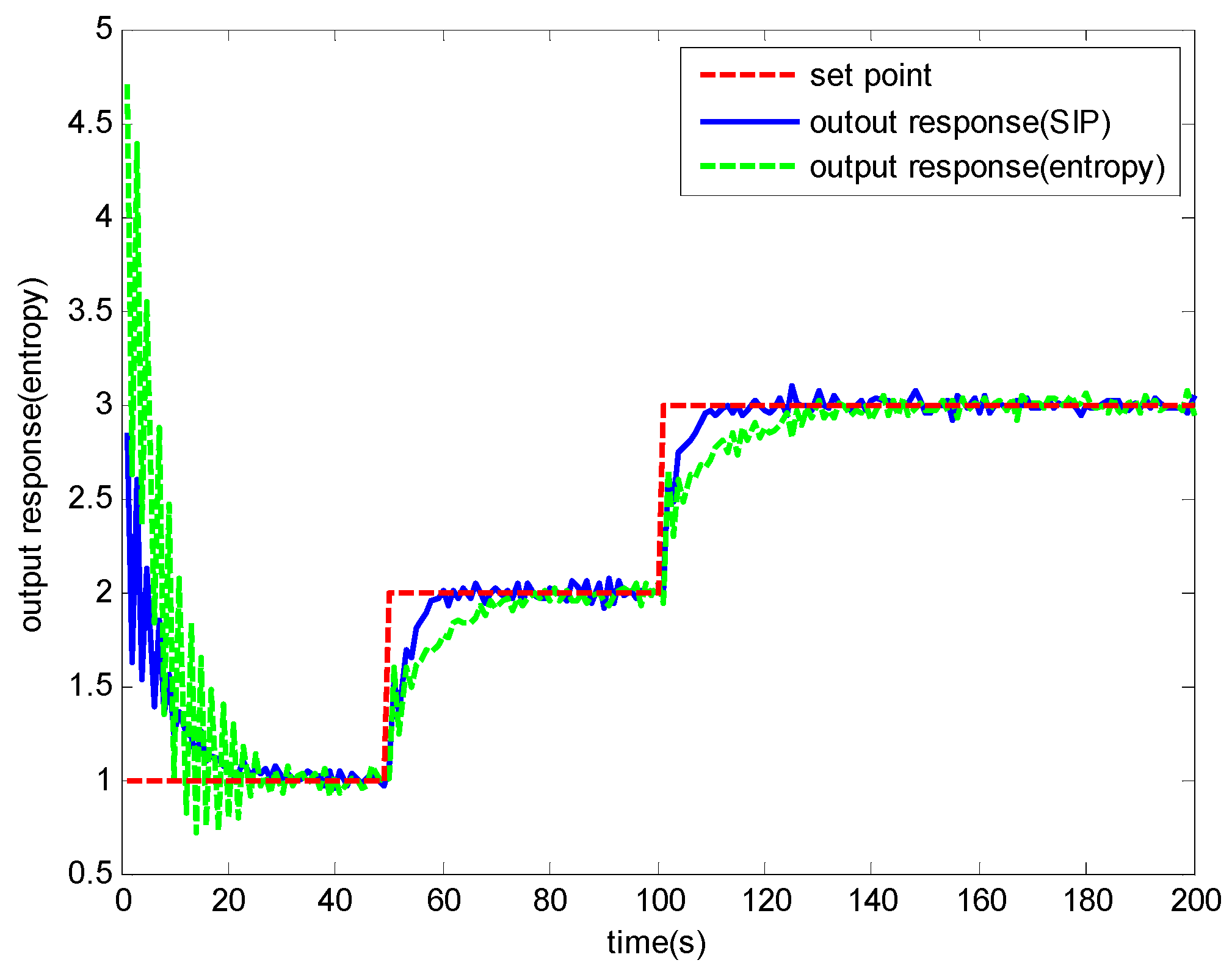
In this simulation, the corresponding control inputs based on SIP and entropy criteria respectively are implemented on the system Equation (38) at each time point. Some comparative results are given to illustrate the superiority of the proposed SIP based stochastic predictive tracking control algorithm. In Figure 1, it is clear that the proposed control algorithm based on the SIP criterion has better performance, the fluctuation of the output response is smaller, and the response is quicker using the SIP method. 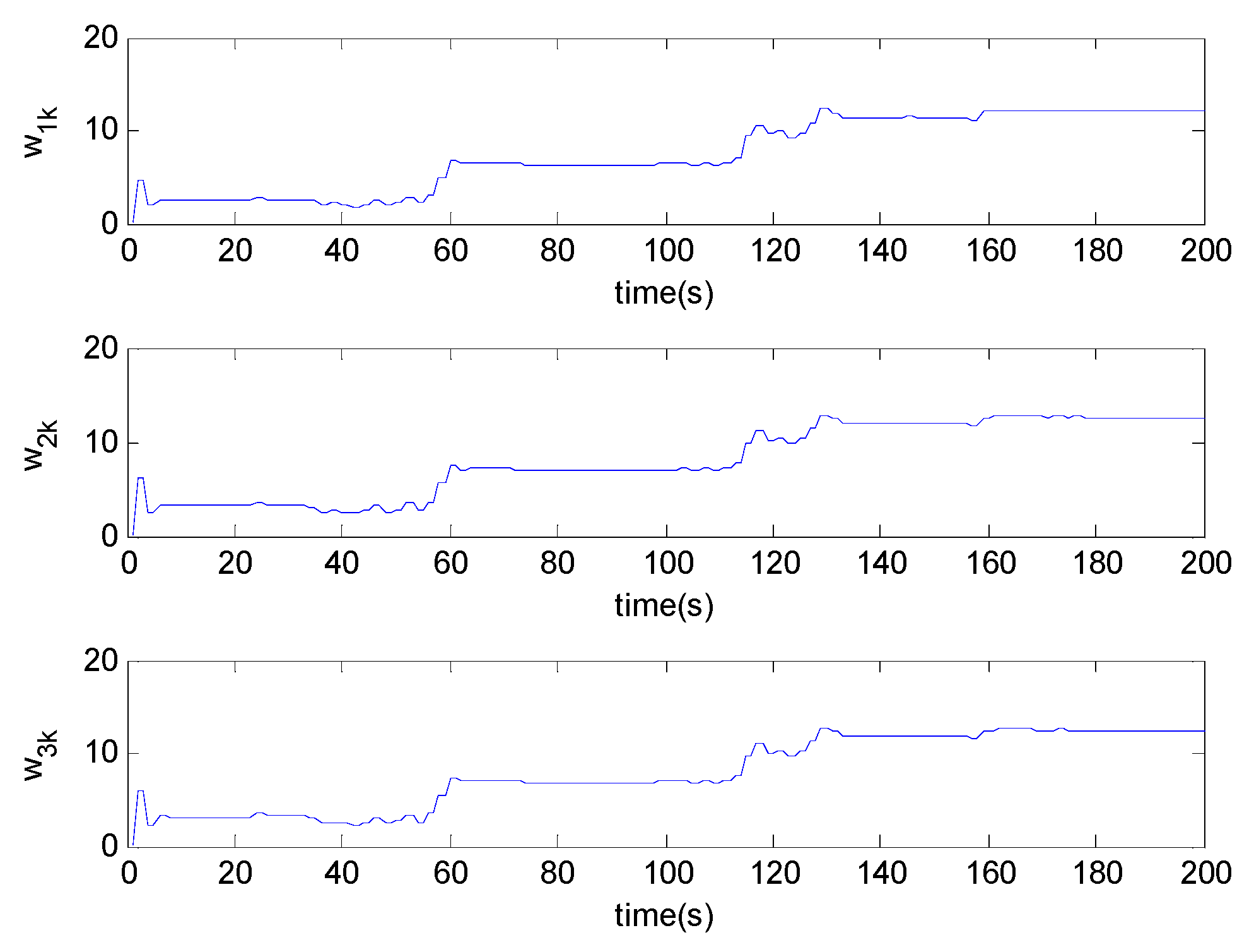In Figure 2, the trend of the performance index Equation (9) is presented. It is found that the performance index is overall decreasing with the progress of the time although some small variations can be recorded. The variances of the single neuron weights are presented in Figure 3. 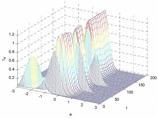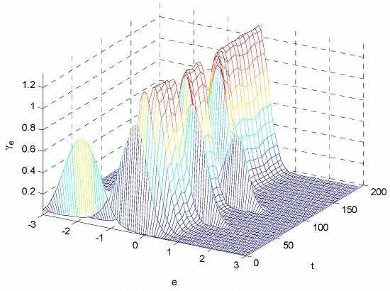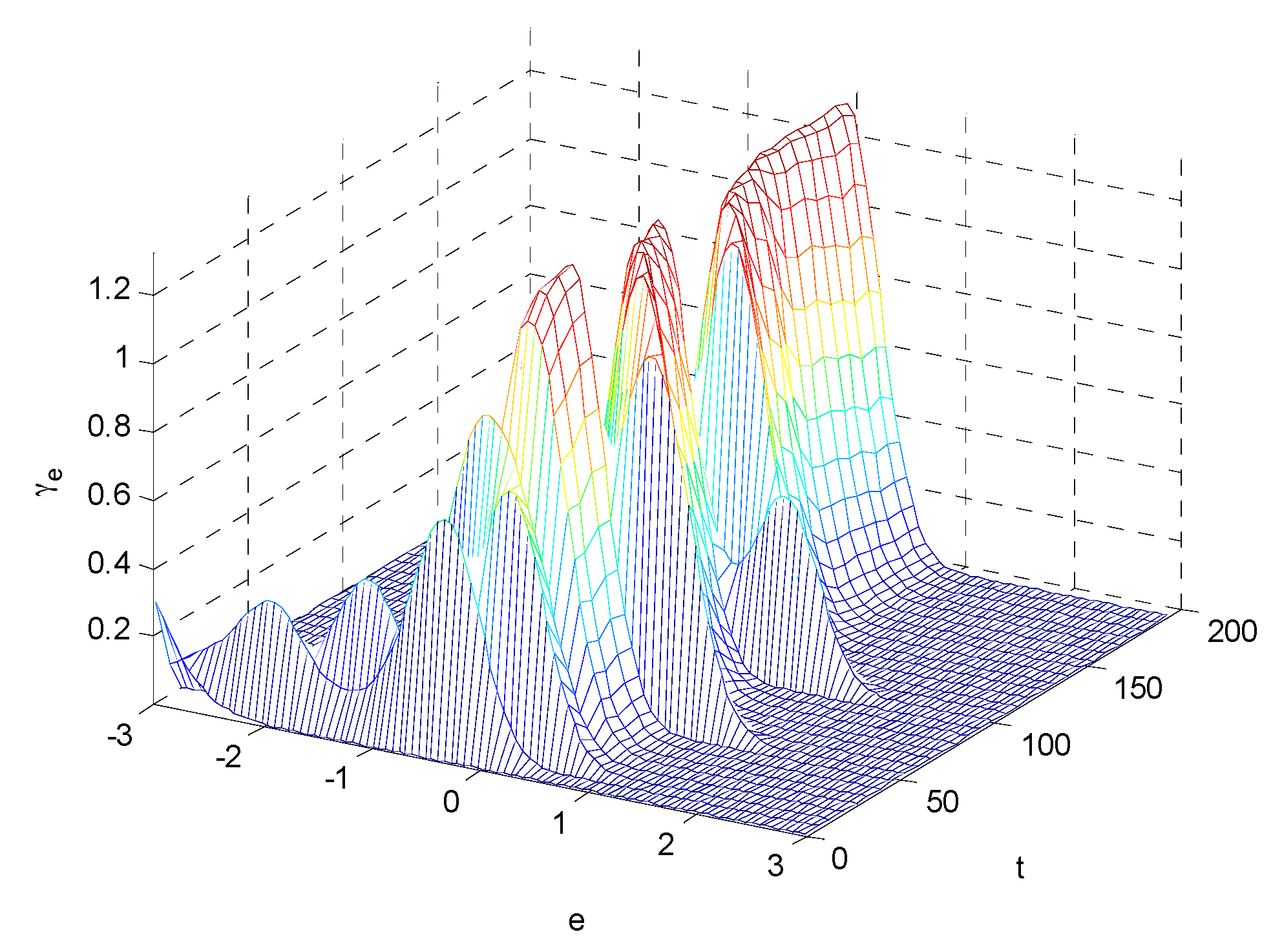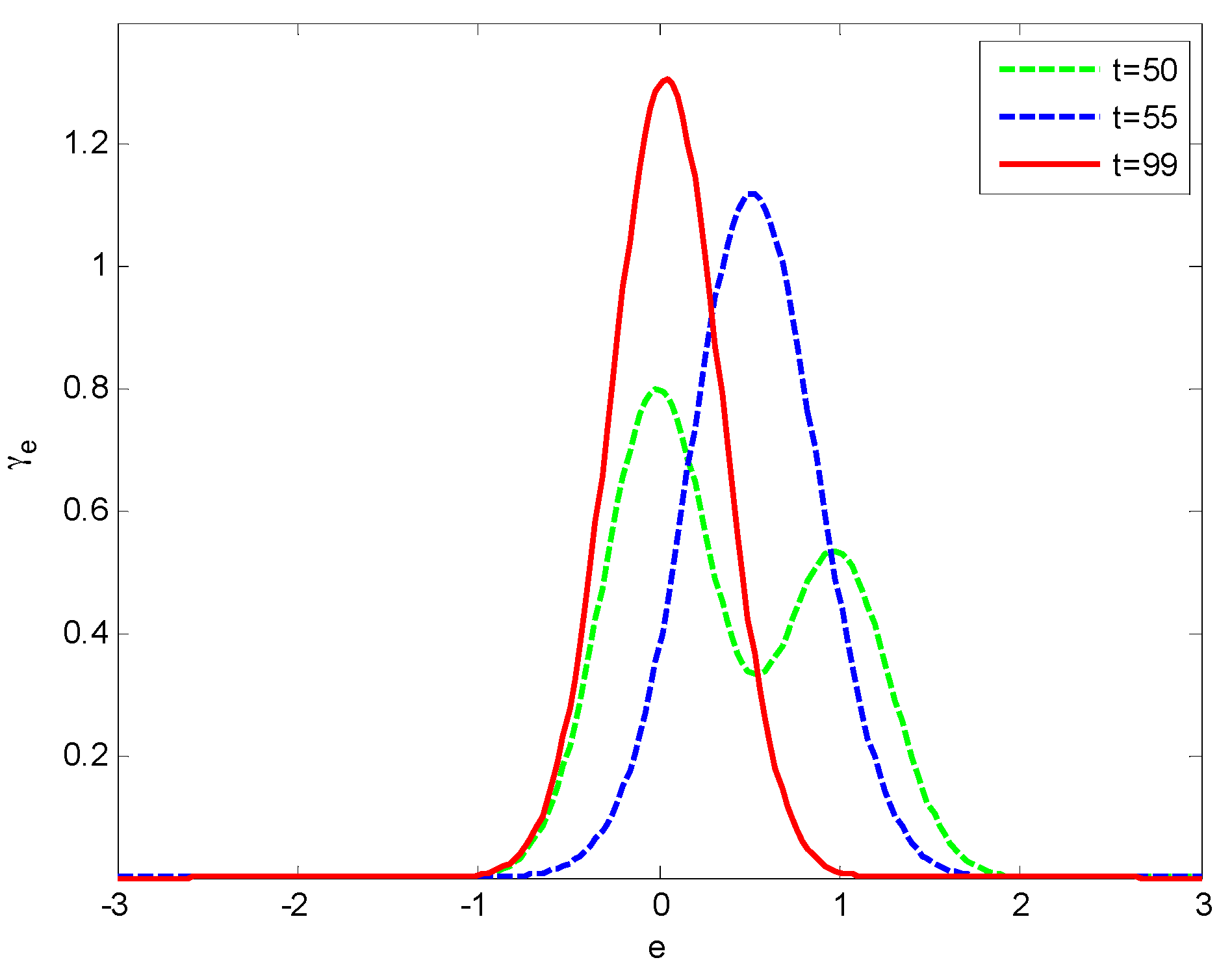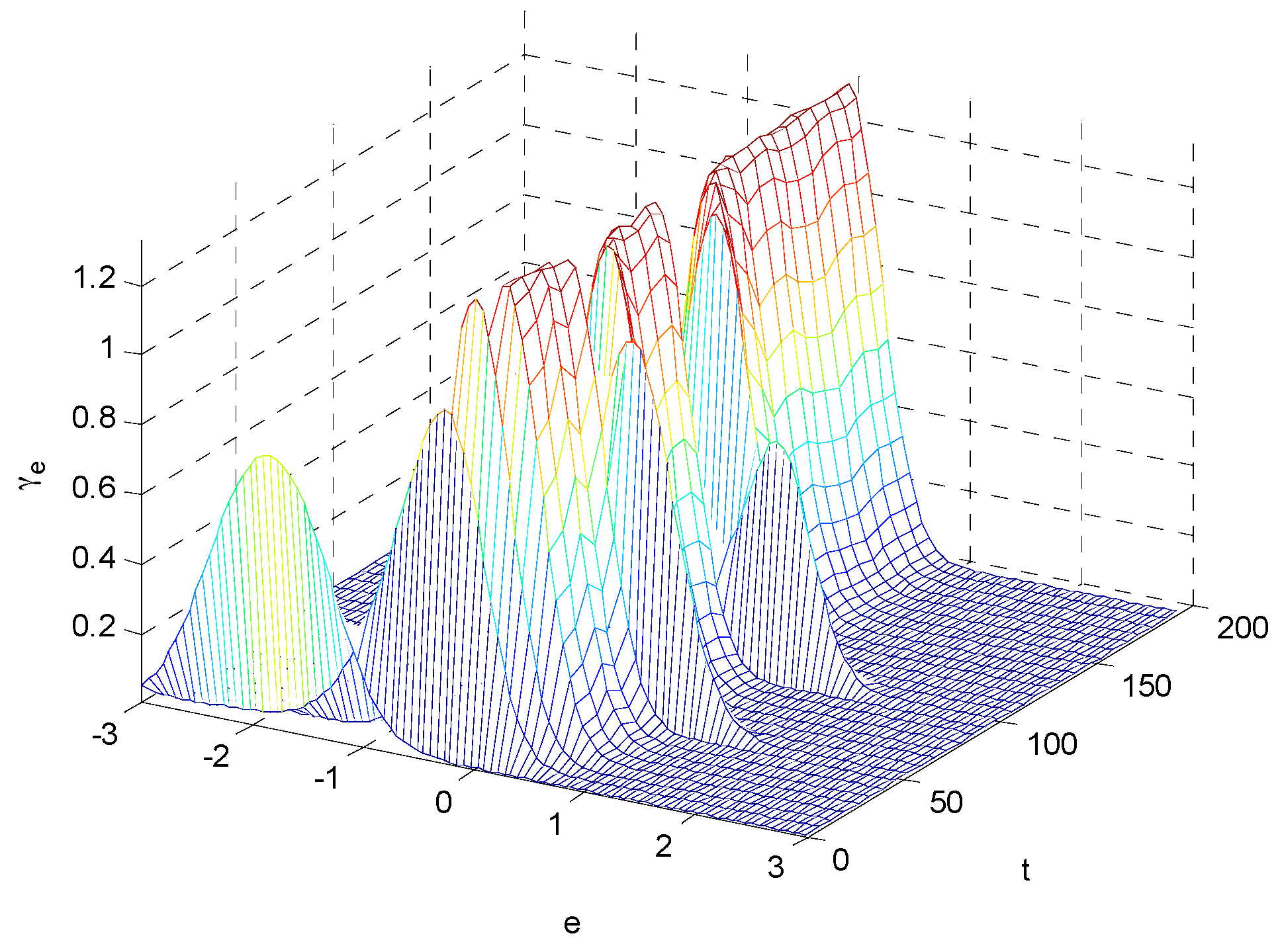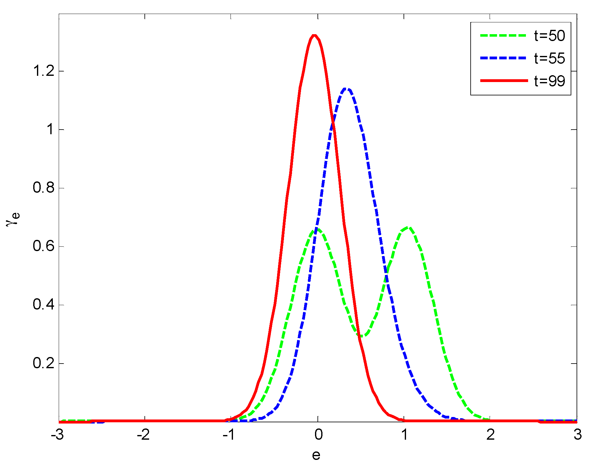Figure 4 and Figure 5 demonstrate the PDFs of the output tracking errors using the entropy-based controller, while Figure 6 and Figure 7 illustrate the PDFs of the tracking errors using the proposed SNSPC method. Compared with Figure 4, the shape of the PDF of the tracking error in Figure 6 turns to be narrower and sharper over the control process, which indicates that the proposed SNSPC control system has achieved a smaller uncertainty in the tracking error distribution. In addition, it can also be seen that the peak of the tracking error PDF locates in the vicinity of zero using the proposed method. In Figure 8, the final PDF of the tracking error under the proposed control law is sharper and narrower than that under the entropy-based control law.

5. Conclusions

In the past, several different approaches, such as PDF shaping control, minimum entropy control, generalized minimum entropy control, etc. have been proposed to solve the control problem for non-Gaussian stochastic systems. These control strategies can achieve good performance, but there are still two main issues to be further improved: (1) The entropy value can be negative and it is shift-invariant. More suitable statistical information that describes objective functions is necessary; (2) Control input in a stochastic system is also a random variable. The randomness of control input should be considered.

In this work, a convergent SNSPC algorithm is presented for the controlled system with non-Gaussian disturbance. The proposed SNSPC is obtained by minimizing a SIP-based predictive criterion, in which the randomness of the control input is also considered besides randomness of the tracking error. Compared with the entropy or IP, the randomness measure SIP has some advantages, such as validity in a wide range of distributions, robustness, and the simplicity in computation. Moreover, the multistep predictive control strategy, rather than single step control is developed in this paper as it is more robust to disturbances and nonlinearities involved in the systems. Also, the convergent condition of the proposed SNSPC based on the energy conservation principle is proposed. The proposed control strategy is applied in a nonlinear and non-Gaussian stochastic numerical example. The simulation results confirm that this new SIP based predictive control method can achieve a good tracking performance.

Compared with the previous work in the field of stochastic distribution control, the contributions of this paper are three folds: (1) the randomness of control inputs is considered for the first time; (2) instead of the instantaneous performance index, a novel SIP-based cumulative criterion is formulated; (3) a single neuron multi-step predictive control algorithm is obtained, and it is much better than the single-step control method. However, most of the practical industrial processes have multi-inputs and multi-outputs, and there are also many constraints when the controller is designed. Future research should be focused on such problems.