Entropy Generation on Nanofluid Flow through a Horizontal Riga Plate

Abstract

In this article, entropy generation on viscous nanofluid through a horizontal Riga plate has been examined. The present flow problem consists of continuity, linear momentum, thermal energy, and nanoparticle concentration equation which are simplified with the help of Oberbeck-Boussinesq approximation. The resulting highly nonlinear coupled partial differential equations are solved numerically by means of the shooting method (SM). The expression of local Nusselt number and local Sherwood number are also taken into account and discussed with the help of table. The physical influence of all the emerging parameters such as Brownian motion parameter, thermophoresis parameter, Brinkmann number, Richardson number, nanoparticle flux parameter, Lewis number and suction parameter are demonstrated graphically. In particular, we conferred their influence on velocity profile, temperature profile, nanoparticle concentration profile and Entropy profile.

1. Introduction

During recent years, nanofluids with heat transfer have received much interest due to their wide range of applications in engineering and industrial processes. Such types of applications include: thermal therapy for the treatment of cancer diseases, metallurgical sectors and chemical process, power generation, transportation, micro-production, cooling, heating, air-conditioning, and ventilation. In fact, they depict very high thermal conductivity compared to the conventional coolants, even when the particle concentration is very low. It is very well known that conventional heat transfer is poor in various types of fluids such as ethylene glycol, water, and oil that have lower thermal conductivity. Nanofluids are very helpful in handling the cooling problems in different thermal systems. Such kinds of high thermal conductivity can be useful in the automatic transmission of fluids, lubricants, coolants and engine oils. However, fluids that have lower thermal conductivity can be improved by adding solid nanoparticles. Nanoparticles consist of metallic or nonmetallic particles of nanometer-size in the conventional fluids. Nanofluids are also very much significant and important in nano/microchannel electronic devices, heat exchangers, cooling system in industrial process and evaporators, etc. Nanofluids are secure and do not involve any other issues, i.e., erosion, rheological characteristics, sedimentation and pressure drop, etc. This is due to the fact that a nanoparticle consists of very small nano sized particles. Ahmad et al. [1] studied the viscous fluid flow of nanofluid through a Riga plate to consider the effects of Lorentz force. Kuznetsov and Nield [2] examined the natural convection on boundary layer flow of nanofluid towards a vertical plate. Sheikholeslami et al. [3] explored the simultaneous impact of thermal radiation and MHD on nanofluids using a two phase model with heat transfer. Sheikholeslami and Ganji [4] studied the heat transfer with the combination of copper water nanofluids flow between parallel plates. Zeeshan et al. [5] examined the viscous flow of a nanofluid through concentric cylinders. Pantzali et al. [6] investigated the influence of nanofluids with modulated surface to analyze the performance of a miniature plate heat exchanger. Sheikholeslami and Ellahi [7] studied the impact of electrohydrodynamic nanofluids with the help of hydrothermal treatment through an enclosure with a wavy upper wall. Rahman et al. [8] considered the combined effects of slip and nanoparticles on the non-Newtonian Jeffrey fluid model towards a tapered artery with mild stenosis. Zeeshan et al. [9] considered the influence of magnetic dipole on Newtonian nanofluids through a stretching surface having thermal radiation. Some more relevant studies on this topic can be found in references [10,11,12,13,14,15].

The study of entropy generation with heat and mass transfer have been investigated by various researchers. In a thermodynamical system, friction forces, diffusion process, and chemical reaction between solid surfaces and fluid viscosity within a system provide an energy loss and entropy generation induction in the system. Different thermal systems are associated with the phenomena of irreversibility which can be defined by entropy generation and is relevant to viscous dissipation function, heat transfer, and mass transfer, etc. To enhance the irreversibilities mechanism, the second law of thermodynamics is a well known and powerful method that has been utilized by various researchers. However, initially, the first law of thermodynamics was used by many researchers and they observed that it is not efficient compared to the second law of thermodynamics. Due to this, entropy generation has received a significant interest in various fields such as turbomachinery, heat exchangers, and electronic cooling. Ellahi et al. [16] studied the shape effects of nanoparticles in copper water nanofluids with entropy generation. Zeeshan et al. [17] examined the non-Darcy mixed convection flow under the effect of magnetic field through permeable a stretching surface. He also considered the effects of ohmic heating and obtained a numerical solution with the help of the shooting method. Rashidi et al. [18] investigated the entropy generation in steady MHD flow of nanofluid through a porous rotating disk. They observed that disk is the important source of entropy generation. Nawaz et al. [19] applied the genetic algorithm and Nelder mead method to analyze the influence of Joule and Newtonian heating through a stretching surface. Abolbashari et al. [20] studied the entropy generation on unsteady MHD flow of nanofluid towards a permeable stretching surface. Later, Abolbashari et al. [21] investigated analytically the entropy generation on Casson nanofluid past a stretching surface. Qing et al. [22] studied numerically the entropy generation on MHD Casson nanofluid through a porous stretching surface. They found that entropy generation enhances due to the influence of all the physical parameters. Some more pertinent studies on this topic can be found in references [23,24,25]. According to the best of our knowledge, entropy generation on viscous nanofluid flow through a horizontal Riga plate has not been reported before.

Drawing motivation from the above studies, the aim of the present study is to analyze the entropy generation on viscous nanofluid flow through a horizontal Riga plate. The governing flow problem is modeled by taking the approximation of Oberbeck-Boussinesq. Numerical solution has been obtained by means of shooting method (SM) of the coupled nonlinear partial differential equations. The physical influence of all the parameters is discussed with the help of graphs and tables. This paper is summarized in the following way; after the introduction in Section 1. Mathematical formulation of governing flow problem is described in Section 2. Section 3 deals with the formulation of entropy generation. Section 4 characterize the solution methodology and finally, Section 5 is devoted to the graphical and numerical results.

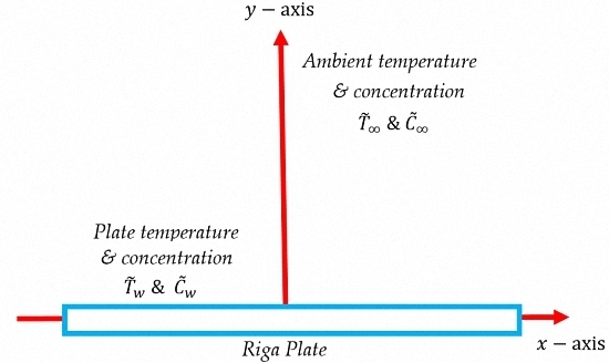
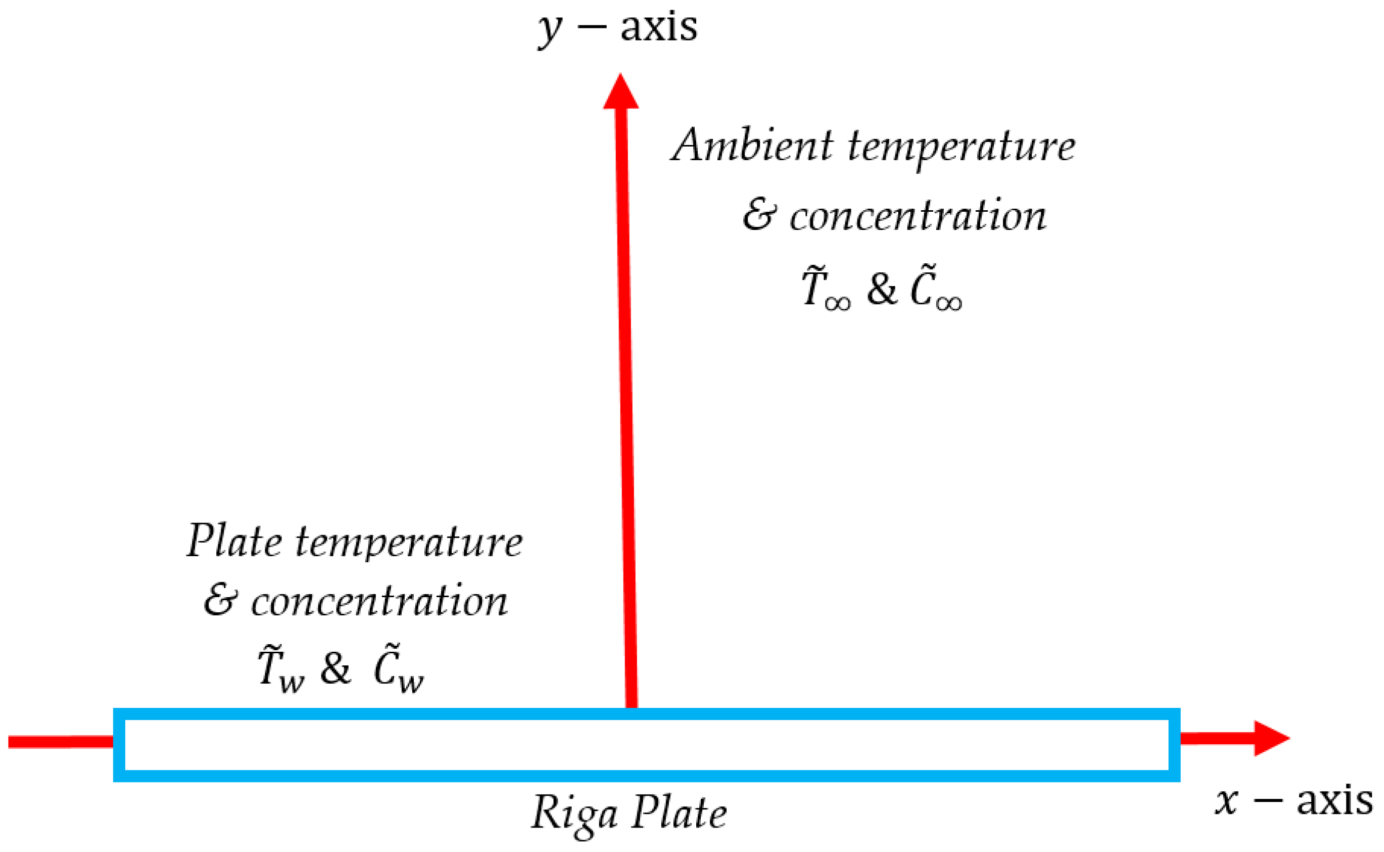
2. Mathematical Formulation

Let us consider the viscous flow of nanofluids with mixed convection boundary layer flow induced by a Riga plate situated at $y=0$ and taking the $x$-axis along the axial direction. The plate is moving with a constant velocity in a viscous nanofluid with suction velocity ${\tilde{v}}_0$. The temperature $(\tilde{T})$ and nanoparticle concentration $(\tilde{C})$ of the sheet have constant values ${\tilde{T}}_w$ and ${\tilde{C}}_w$, respectively. The ambient temperature and nanoparticle concentration are denoted as ${\tilde{T}}_{\infty }$ and ${\tilde{C}}_{\infty }$ as shown in Figure 1.

With the help of Oberbeck-Boussinesq approximation, let us consider that nanoparticle is dilute, and then the boundary layer equations for continuity, linear momentum, thermal energy and concentration equation can be written as [24]

$$\frac{\partial \tilde{u}}{\partial \tilde{x}}+\frac{\partial \tilde{v}}{\partial \tilde{y}}=0,$$

(1)

$$\tilde{u}\frac{\partial \tilde{u}}{\partial \tilde{x}}+\tilde{v}\frac{\partial \tilde{v}}{\partial \tilde{y}}=\frac{\mu }{{\rho }_f}\frac{{\partial }^2\tilde{u}}{\partial {\tilde{y}}^2}+(1+{\tilde{\varphi }}_{\mathsf{\infty }})g{\beta }^{*}(\tilde{T}-{\tilde{T}}_{\mathsf{\infty }})-\frac{{\mathsf{\rho }}_p-{\mathsf{\rho }}_f}{{\mathsf{\rho }}_f}(\tilde{\mathsf{\varphi }}-{\tilde{\mathsf{\varphi }}}_{\mathsf{\infty }}),$$

(2)

$$\tilde{u}\frac{\partial \tilde{T}}{\partial \tilde{x}}+\tilde{v}\frac{\partial \tilde{T}}{\partial \tilde{y}}=\overline{\mathsf{\alpha }}\frac{{\partial }^2\tilde{T}}{\partial {\tilde{y}}^2} +\mathsf{\tau }\left(D_B\frac{\partial \tilde{C}}{\partial \tilde{y}}\frac{\partial \tilde{T}}{\partial \tilde{y}}+\frac{D_T}{T_{\mathsf{\infty }}}{\left(\frac{\partial \tilde{T}}{\partial \tilde{y}}\right)}^2\right),$$

(3)

$$\tilde{u}\frac{\partial \tilde{C}}{\partial \tilde{x}}+\tilde{v}\frac{\partial \tilde{C}}{\partial \tilde{y}}=D_B\frac{{\partial }^2\tilde{C}}{\partial {\tilde{y}}^2}+\frac{D_T}{T_{\infty }}\frac{{\partial }^2\tilde{T}}{\partial {\tilde{y}}^2}.$$

(4)

With their respective boundary conditions are

$$\tilde{u}=u_w, v=v_w, \tilde{T}={\tilde{T}}_w, \tilde{C}={\tilde{C}}_w\text{ at }\tilde{y}=0,$$

(5)

$$\tilde{u}=0, \tilde{T}\to {\tilde{T}}_{\mathsf{\infty }}, \tilde{C}\to {\tilde{C}}_{\mathsf{\infty }} as \tilde{y}\to \mathsf{\infty }.$$

(6)

In the above equations, $\left(\tilde{u},\tilde{v}\right)$ are in the velocity components in $\tilde{x}$-axis and $\tilde{y}$-axis respectively, ${\mathsf{\rho }}_f$ is the density of base fluid, $\mathsf{\mu }, \overline{\mathrm{\alpha }}$ and ${\beta }^{*}$are fluid viscosity, thermal conductivity and volumetric volume coefficient of the nanofluid, ${\mathsf{\rho }}_p$ is the density of the particles. Moreover, $D_B$ and $D_T$ are the Brownian motion and thermos diffusion coefficients and $\overline{\mathsf{\alpha }}$ and $\mathsf{\tau }$ are defined as

$$\overline{\mathsf{\alpha }}=\frac{k}{{\left(\mathsf{\rho }c\right)}_f},\mathsf{\tau }=\frac{{\left(\mathsf{\rho }c\right)}_p}{{\left(\mathsf{\rho }c\right)}_f}.$$

(7)

Let us consider the following non-dimensional quantities

$$\begin{array}{l}\tilde{x}=xl,\tilde{y}=yl,u{u}_w=\tilde{u},v{\tilde{v}}_0=\tilde{v},\mathsf{\theta }=\frac{\tilde{T}-{\tilde{T}}_{\mathsf{\infty }} }{{\tilde{T}}_w-{\tilde{T}}_{\mathsf{\infty }}},\mathsf{\varphi }=\frac{\tilde{C}-{\tilde{C}}_{\mathsf{\infty }} }{{\tilde{C}}_w-{\tilde{C}}_{\mathsf{\infty }}},l\nu =u_w{L}^2,{\tilde{v}}_{0}a=\nu \mathsf{\pi },\\ \mathsf{\lambda }=\frac{a^2\mathrm{\Delta }\tilde{T}}{{\mathsf{\pi }}^2\nu u_w}\left(1-{\tilde{\varphi }}_{\mathsf{\infty }}\right)g{\mathsf{\beta }}^{*},N_R=\frac{a^2\mathrm{\Delta }\tilde{\varphi }}{{\mathsf{\pi }}^2\nu u_w}g\left(\frac{{\mathsf{\rho }}_p-{\mathsf{\rho }}_f}{{\mathsf{\rho }}_f}\right),z=\frac{a^2{j}_0{M}_0}{8\mathsf{\pi }\nu u_w{\mathsf{\rho }}_f},N_b=\frac{\mathsf{\tau }{D}_B\mathrm{\Delta }\varphi }{\nu },\\ N_t=\frac{\mathsf{\tau }{D}_T\mathrm{\Delta }\tilde{T}}{\nu {\tilde{T}}_{\mathsf{\infty }}}, \nu =\frac{\mathsf{\mu }}{{\mathsf{\rho }}_f}, {\mathrm{P}}_{\mathrm{r}}=\frac{v}{\overline{\alpha }}, L_e=\frac{\nu }{D_B}.\end{array}$$

(8)

Using Equation (8) in to Equations (2)–(6), we get

$$u\frac{\partial u}{\partial x}+v\frac{\partial v}{\partial y}-\frac{{\partial }^{2}u}{\partial y^2}+N_R\mathsf{\varphi }-\mathsf{\lambda }\mathsf{\theta }=0,$$

(9)

$$u\frac{\partial \mathsf{\theta }}{\partial x}+v\frac{\partial \mathsf{\theta }}{\partial y}-\frac{1}{P_r}\frac{{\partial }^2\mathsf{\theta }}{\partial y^2}-N_b\frac{\partial \mathsf{\theta }}{\partial y}\frac{\partial \mathsf{\varphi }}{\partial y}-N_t{\left(\frac{\partial \mathsf{\theta }}{\partial y}\right)}^2=0,$$

(10)

$$u\frac{\partial \mathsf{\varphi }}{\partial x}+v\frac{\partial \mathsf{\varphi }}{\partial y}-\frac{1}{L_e}\frac{{\partial }^2\mathsf{\varphi }}{\partial y^2}-\frac{N_t}{L_e{N}_b}\frac{{\partial }^2\mathsf{\theta }}{\partial y^2}=0.$$

(11)

Their boundary conditions takes the new form

$$u=1, v=v_w, \mathsf{\theta }=1, \mathsf{\varphi }=1 \text{at }y=0,$$

(12)

$$u\to 0, \mathsf{\theta }=0, \mathsf{\varphi }=0 at y\to \mathsf{\infty },$$

(13)

where $\mathsf{\lambda }$ is the Richardson number, $N_t$ is the thermophoresis parameter, $N_R$ is the nanoparticle concentration flux parameter, $\nu$ is the kinematic viscosity, ${\mathrm{P}}_r$ is the Prandtl number, $L_e$ is the Lewis number, $N_b$ is the Brownian motion parameter, respectively. Using the assumption of strong suction, the problem can be re-written in the following form as

$$\frac{\partial v}{\partial y}=0,$$

(14)

$$v\frac{\partial u}{\partial y}-\frac{{\partial }^{2}u}{\partial y}-\mathsf{\lambda }\mathsf{\theta }+N_R\mathsf{\varphi }=0,$$

(15)

$$u\frac{\partial \mathsf{\theta }}{\partial x}+v\frac{\partial \mathsf{\theta }}{\partial y}-\frac{1}{{\mathrm{P}}_{\mathrm{r}}}\frac{{\partial }^2\mathsf{\theta }}{\partial y^2}-N_b\frac{\partial \mathsf{\theta }}{\partial y}\frac{\partial \varphi }{\partial y}-N_t{\left(\frac{\partial \mathsf{\theta }}{\partial y}\right)}^2=0,$$

(16)

$$u\frac{\partial \mathsf{\varphi }}{\partial x}+v\frac{\partial \mathsf{\varphi }}{\partial y}-\frac{1}{L_e}\frac{{\partial }^2\mathsf{\varphi }}{\partial y^2}-\frac{N_t}{L_e{N}_b}\frac{{\partial }^2\mathsf{\theta }}{\partial y^2}=0.$$

(17)

With the help of continuity equation and the corresponding condition$v\left(0\right)=v_w$, the governing equations can be rewritten as

$$v_w\frac{\partial u}{\partial y}-\frac{{\partial }^{2}u}{\partial y}-\mathsf{\lambda }\mathsf{\theta }+N_R\mathsf{\varphi }=0,$$

(18)

$$v_w\frac{\partial \mathsf{\theta }}{\partial y}-\frac{1}{{\mathrm{P}}_{\mathrm{r}}}\frac{{\partial }^2\mathsf{\theta }}{\partial y^2}-N_b\frac{\partial \mathsf{\theta }}{\partial y}\frac{\partial \mathsf{\varphi }}{\partial y}-N_t{\left(\frac{\partial \mathsf{\theta }}{\partial y}\right)}^2=0,$$

(19)

$$v_w\frac{\partial \mathsf{\varphi }}{\partial y}-\frac{1}{L_e}\frac{{\partial }^2\mathsf{\varphi }}{\partial y^2}-\frac{N_t}{L_e{N}_b}\frac{{\partial }^2\mathsf{\theta }}{\partial y^2}=0.$$

(20)

The physical quantities of interest for the governing flow problem are local Nusselt number and local Sherwood number in dimensionless form can be written as [21]

$$N{u}_x=-{\mathsf{\theta }}^{\prime }\left(0\right), S{h}_x=-{\mathsf{\varphi }}^{\prime }\left(0\right).$$

(21)

3. Entropy Generation Analysis

The volumetric entropy generation of the viscous fluid is given by [25]

$$S_{gen}^{‴}=\frac{k}{{\tilde{T}}_{\mathsf{\infty }}^2}{\left(\frac{\partial \tilde{T}}{\partial \tilde{y}}\right)}^2+\frac{{\mathsf{\mu }}_f}{{\tilde{T}}_{\mathsf{\infty }}}{\left(\frac{\partial \tilde{u}}{\partial \tilde{y}}\right)}^2+\frac{RD}{C_{\mathsf{\infty }}}{\left(\frac{\partial \tilde{C}}{\partial \tilde{y}}\right)}^2+\frac{RD}{{\tilde{T}}_{\mathsf{\infty }}}\left(\frac{\partial \tilde{T}}{\partial \tilde{y}}\frac{\partial \tilde{C}}{\partial \tilde{y}}\right).$$

(22)

In the above equation, entropy generation is due to the two factors, (a) conduction effect which is also known as Heat Transfer Irreversibility (HTI); (b) Fluid friction Irreversibility (FFI) and (c) Diffusive irreversibility (DI). The characteristics entropy generation can be described as

$$S_0^{‴}=\frac{k{\left(\mathrm{\Delta }\tilde{T}\right)}^2}{l^2{\tilde{T}}_{\mathsf{\infty }}^2}.$$

(23)

The entropy generation in dimensionless form can be written as

$$N_G=\frac{S_{gen}^{‴}}{S_0^{‴}}={\left(\frac{\partial \mathsf{\theta }}{\partial y}\right)}^2+\frac{{\mathrm{B}}_{\mathrm{r}}}{\mathsf{\Omega }}{\left(\frac{\partial u}{\partial y}\right)}^2+\Lambda {\left(\frac{\mathsf{\Gamma }}{\mathsf{\Omega }}\right)}^2{\left(\frac{\partial \mathsf{\varphi }}{\partial y}\right)}^2+\Lambda \left(\frac{\mathsf{\Gamma }}{\mathsf{\Omega }}\right)\left(\frac{\partial \mathsf{\varphi }}{\partial y}\frac{\partial \mathsf{\theta }}{\partial y}\right),$$

(24)

where ${\mathrm{B}}_{\mathrm{r}}$ is the Brinkmann number and $\mathsf{\Omega }$ and $\mathsf{\zeta }$ are the dimensionless temperature and concentration difference and $\Lambda$ is the diffusion coefficient, respectively. These numbers are given in the following form

$${\mathrm{B}}_{\mathrm{r}}=\frac{{\mathsf{\mu }}_f{u}_w^2}{k\mathrm{\Delta }\tilde{T}}, \mathsf{\Omega }=\frac{\mathrm{\Delta }\tilde{T}}{{\tilde{T}}_{\mathsf{\infty }}}, \mathsf{\Gamma }=\frac{\mathrm{\Delta }\tilde{\mathrm{C}}}{{\tilde{\mathrm{C}}}_{\mathsf{\infty }}}, \Lambda =\frac{RD}{{\tilde{C}}_{\mathsf{\infty }}}.$$

(25)

4. Numerical Method

We apply the shooting method in Equations (18)–(20) with their boundary conditions in Equations (12) and (13). Initially, Equations (18)–(20) reduces to initial value problem in the following form

$$\frac{\partial u}{\partial y}=U_1, \frac{\partial U_1}{\partial y}=v_w{U}_1-\mathsf{\lambda }\mathsf{\theta }+N_R\mathsf{\varphi }$$

(26)

$$\frac{\partial \mathsf{\theta }}{\partial y}=U_2, \frac{\partial U_2}{\partial y}={\mathrm{P}}_{\mathrm{r}}\left(v_w{U}_2-N_b{U}_3{U}_2-N_t{U}_2^2\right),$$

(27)

$$\frac{\partial \mathsf{\varphi }}{\partial y}=U_3, \frac{\partial U_3}{\partial y}=L_e\left(v_w{U}_3-\frac{N_t}{N_b{L}_e}\frac{\partial U_2}{\partial y}\right).$$

(28)

Along with their boundary conditions

$$u=1, U_1=S_1, \mathsf{\theta }=1, U_2=S_2, \mathsf{\varphi }=1, U_3=S_3\text{ at }y=0,$$

(29)

where for the suction velocity we take$v_w=-s\left(s>0\right)$. To solve the above equations, a suitable initial guess is chosen for $S_1, S_2$ and $S_3$ for numerical computations. The step size is chosen $\mathrm{\Delta }y=0.001$ and $y_{\mathsf{\infty }}=3$ at their given boundary conditions.

5. Numerical Results and Discussion

This section deals with numerical and graphical results of all the emerging parameters involved in the governing flow problem. For this purpose, Figure 2, Figure 3, Figure 4, Figure 5, Figure 6, Figure 7, Figure 8, Figure 9, Figure 10 and Figure 11 are sketched against velocity, temperature, nanoparticle concentration and entropy profile. In particular, the influence of Brownian motion parameter, thermophoresis parameter, Richardson number, Prandtl number, nanoparticle flux parameter, Lewis number, Brinkmann number, suction parameter, Brinkmann number and entropy parameters respectively are taken into account. Furthermore, the expression for Nusselt number and Sherwood number are also undertaken for different values of Prandtl number, Lewis number, Brownian motion parameter and thermophoresis parameter as given in

Table 1. Numerical values of reduced Nusselt number $\left(N{u}_x\right)$ and Sherwood number $\left(S{h}_x\right)$ for various values of${\mathrm{P}}_{\mathrm{r}}, L_e, N_b \text{and }{N}_t$.

$P_r$	${\mathit{L}}_{\mathit{e}}$	${\mathit{N}}_{\mathit{b}}$	${\mathit{N}}_{\mathit{t}}$	$\mathit{N}{\mathit{u}}_{\mathit{x}}$	$\mathit{S}{\mathit{h}}_{\mathit{x}}$
$1$	$1$	$0.3$	$0.3$	$3.1759$	$0.8204$
$1.5$	-	-	-	$4.5276$	$-0.5339$
$2$	-	-	-	$5.8211$	$-1.8261$
-	$2$	-	-	$2.9494$	$5.0388$
-	$2.5$	-	-	$2.8916$	$7.0573$
-	$3$	-	-	$2.8531$	$8.9940$
-	-	$0.1$	-	$3.5277$	$-6.5947$
-	-	$0.2$	-	$3.3485$	$-1.0285$
-	-	$0.4$	-	$3.0097$	$1.7400$
-	-	-	$0.1$	$3.3422$	$2.8841$
-	-	-	$0.2$	$3.2579$	$1.8250$
-	-	-	$0.4$	$3.0961$	$0.1317$

. From this table, we can see that the influence of thermophoresis parameter causes a reduction in Nusselt number and Sherwood number. Moreover, by increasing Brownian motion parameter, the Nusselt number decreases and Sherwood number increases.

Figure 2 and Figure 3 are sketched for velocity profile against Richardson number $\mathsf{\lambda }$, nanoparticle flux parameter$N_R$, suction parameter $S$ and Prandtl number ${\mathrm{P}}_{\mathrm{r}}$. It depicts from Figure 2 that Richardson $\mathsf{\lambda }$ enhances the velocity profile. In this figure, we can also observe that when $\mathsf{\lambda }=1$ then it is known as buoyancy driven flow and when $\mathsf{\lambda }>1$then buoyancy gets more dominating. Moreover, we can also analyze here that nanoparticle flux parameter $N_R$ opposes the flow and causes a reduction in the velocity profile. From Figure 3, we can analyze that when the suction parameter $S$ increases then the velocity of the fluid decreases. However, Prandtl number ${\mathrm{P}}_{\mathrm{r}}$ shows the opposite behavior and enhances the velocity profile. Physically, the ratio of the thickness is controlled by Prandtl number and we can examine here that when ${\mathrm{P}}_{\mathrm{r}}=1$than both the boundary layer are of same thickness; however, with the increment in Prandtl number ${\mathrm{P}}_{\mathrm{r}}>1,$ the thermal boundary layer gets thinner as compared to the velocity boundary layer.

Figure 4 and Figure 5 are prepared for temperature profile against Brownian motion parameter $N_b$, thermophoresis parameter $N_t$, Prandtl number ${\mathrm{P}}_{\mathrm{r}}$ and suction parameter $S$. It is clear from Figure 4 that thermophoresis parameter $N_t$ enhances the temperature profile and its boundary layer thickness. Moreover, we can also observe here that suction parameter $S$ shows the opposite behavior in temperature profile and causes reduction. It can be observed from Figure 4 that Brownian motion parameter also enhances the temperature and its boundary layer thickness. Here, we can notice that Prandtl number ${\mathrm{P}}_{\mathrm{r}}$ causes a reduction in temperature profile and its boundary layer thickness. In fact, this is due to weaker thermal diffusivity. Those fluids having weaker thermal diffusivity contain lower temperatures, and such kinds of weaker thermal diffusivity diminish the temperature profile and boundary layer thickness.

Figure 6, Figure 7 and Figure 8 are sketched for concentration profile against Lewis number $L_e,$ suction parameter $S$, Brownian motion parameter $N_b$, thermophoresis parameter $N_t$ and Prandtl number ${\mathrm{P}}_{\mathrm{r}}$, respectively. It is depicted in Figure 6 that, with the increment in Lewis number $L_e$ and suction parameter $S$ there tends to be a reduction in the concentration profile and its associated boundary layer thickness. It can be noticed from Figure 7 that Brownian motion parameter $N_b$ causes a reduction in the concentration profile and its related boundary layer thickness, however, Prandtl number ${\mathrm{P}}_r$ shows an enhancement in concentration profile when $\left(y<0.5\right)$, but when $\left(y>0.5\right)$ it causes a decrement in the nanoparticle concentration profile. Figure 8 shows that thermophoresis parameter $N_t$ enhances the nanoparticle concentration profile and its boundary layer thickness. Figure 9, Figure 10 and Figure 11 shows the behavior of entropy profile against different values of $B_r$, $\mathsf{\zeta },\mathsf{\Omega },\mathsf{\Gamma },{\mathrm{P}}_{\mathrm{r}}$ and $S.$ In all these figures we can conclude that all these parameters enhance the entropy profile.

6. Conclusions

In this article, entropy generation on viscous nanofluid through a horizontal Riga plate has been analyzed. The governing flow problem is modeled with the help of Oberbeck-Boussinesq approximation. The resulting nonlinear coupled partial differential equations are solved numerically by means of shooting method (SM). The major outcomes of the present study are summarized below:

(i)

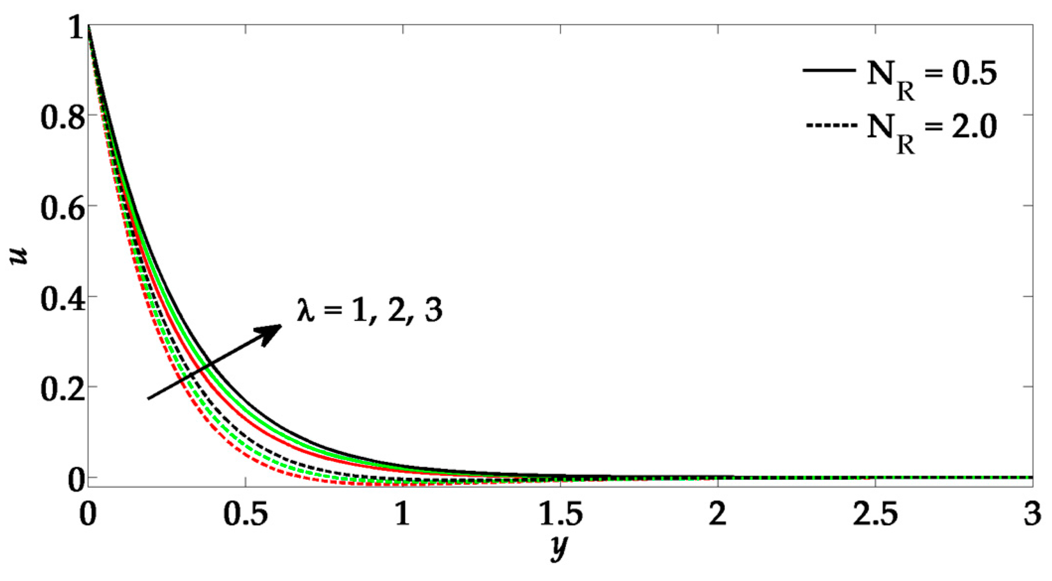
The Richardson number enhances the velocity; however, nanoparticle flux parameter opposes the flow.

(ii)

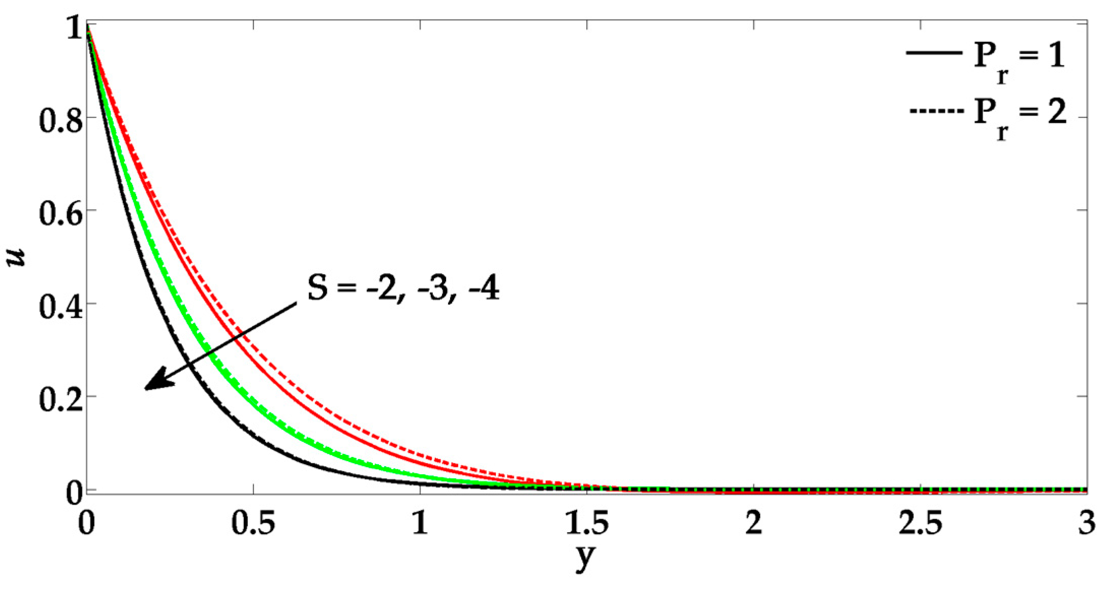
By increasing Prandtl number, the velocity profile tends to rise.

(iii)

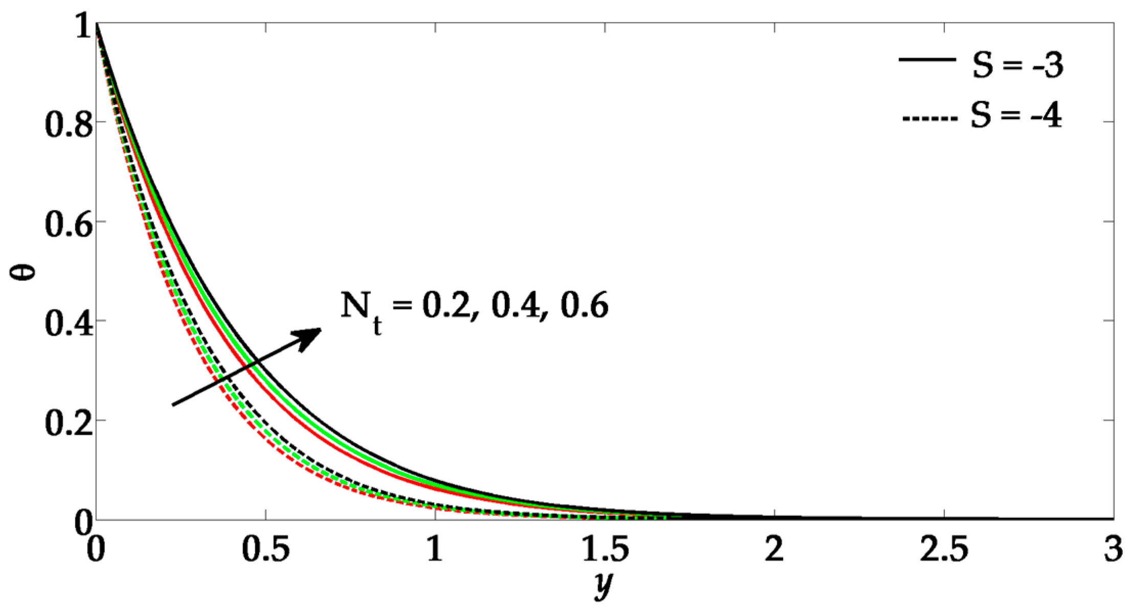
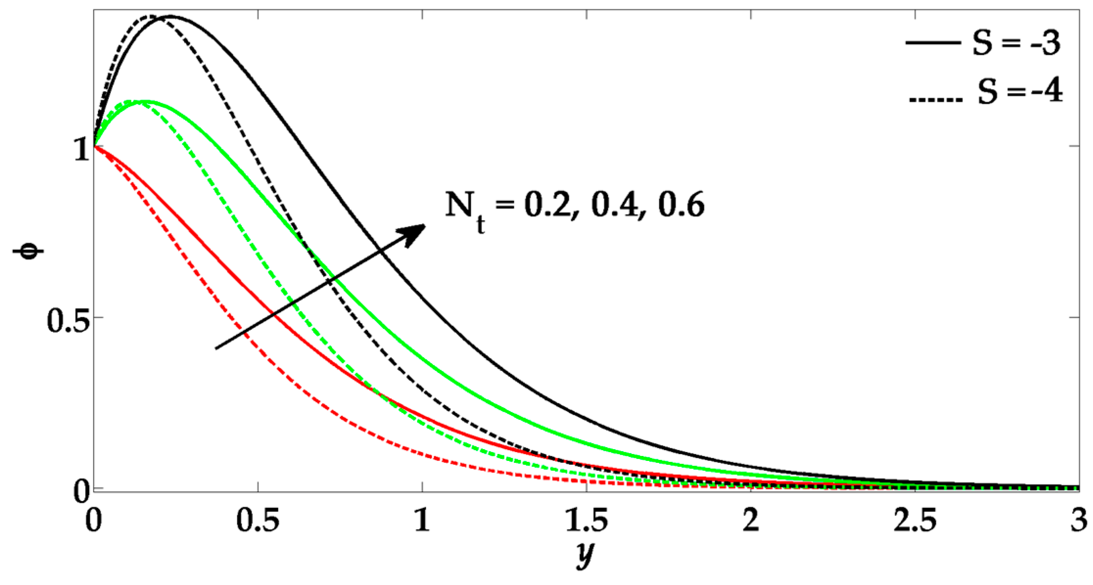
The Brownian motion parameter and thermophoresis parameter also enhances the temperature profile and its boundary layer thickness.

(iv)

Due to a greater influence of Prandtl number and suction parameter, the temperature profile tends to diminish.

(v)

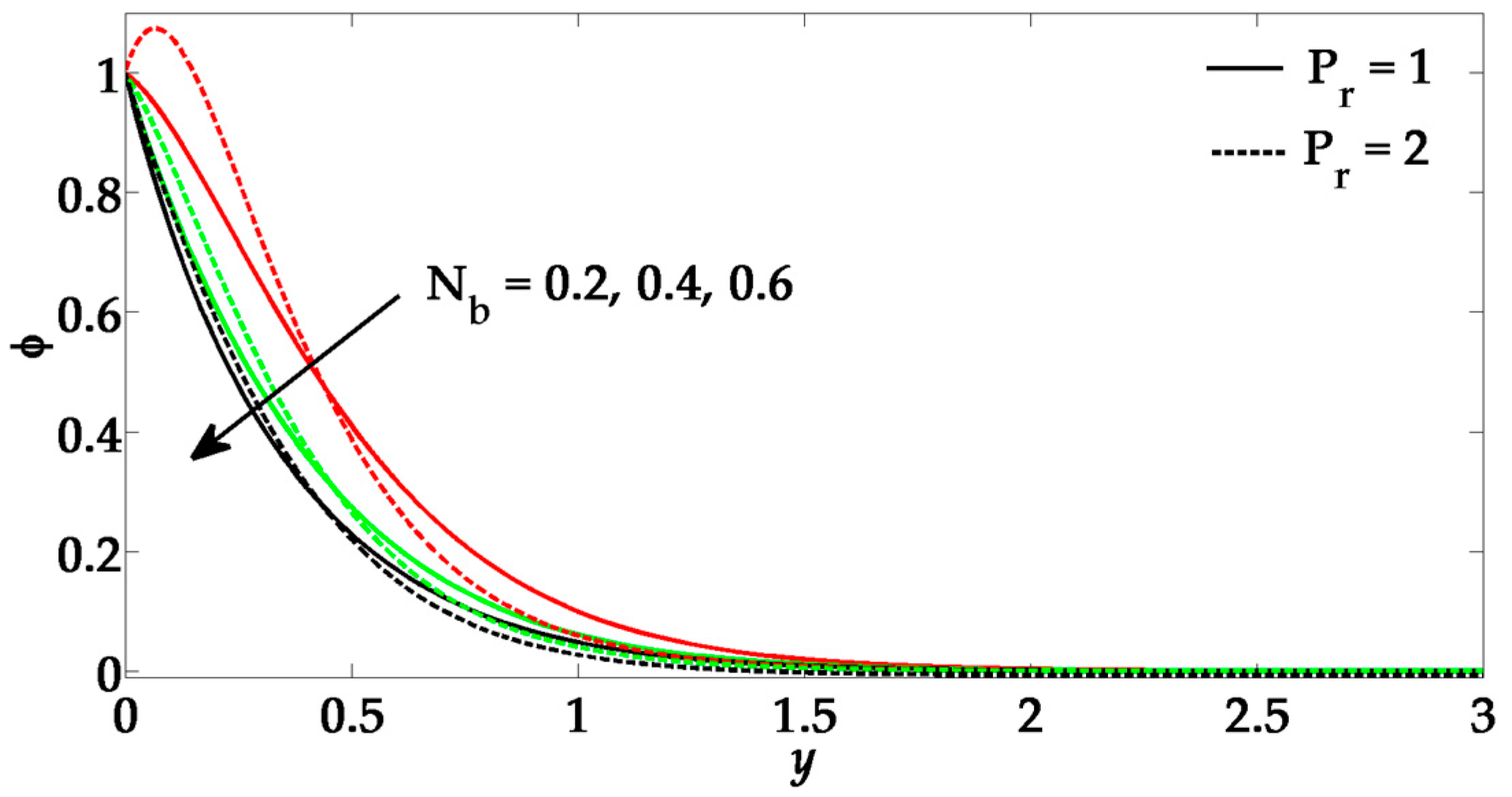
The Prandtl number enhances the nanoparticle concentration profile and its boundary layer thickness.

(vi)

The thermophoresis parameter and Brownian motion parameter show alternate behavior on nanoparticle concentration profile.

(vii)

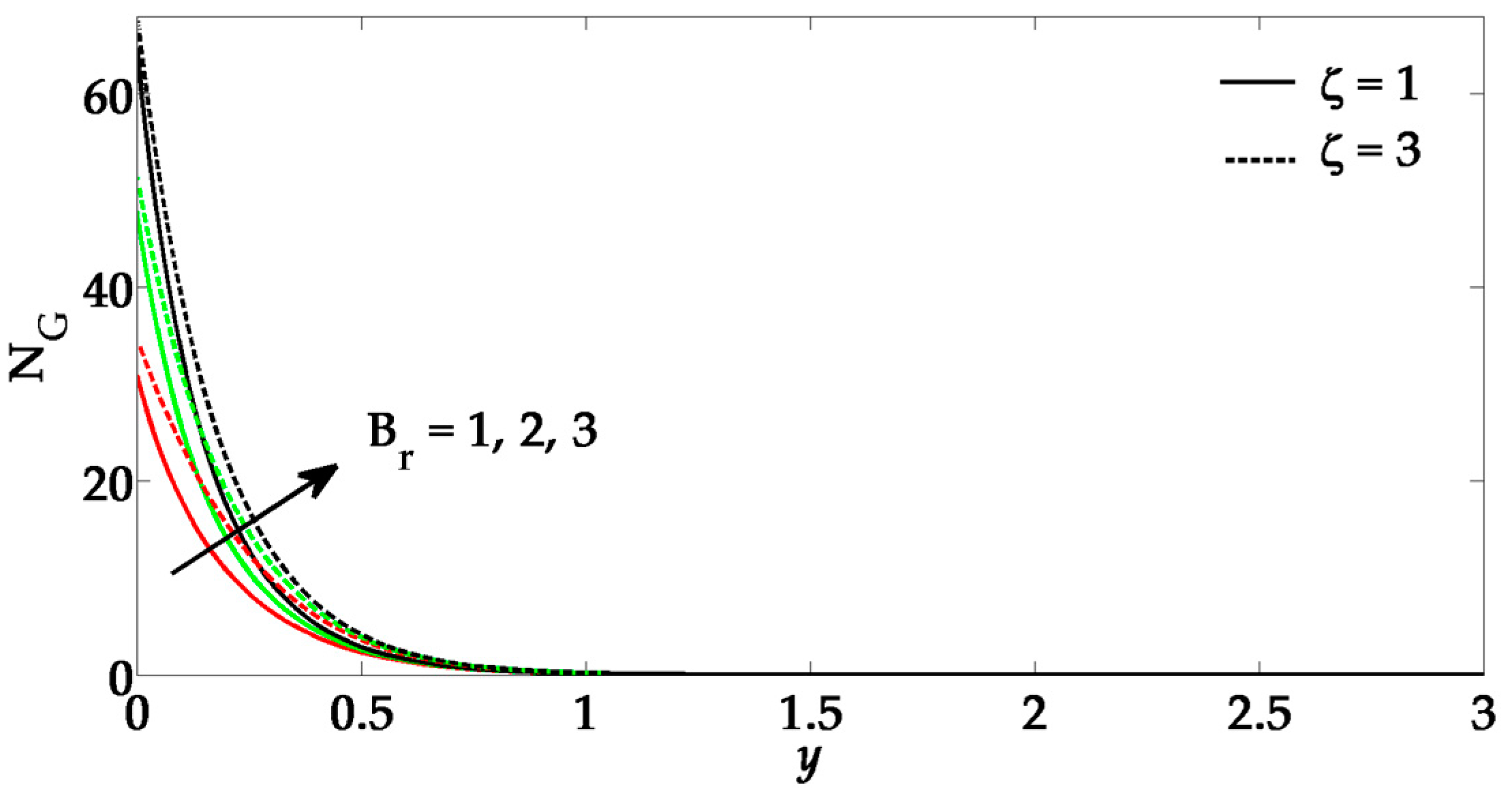
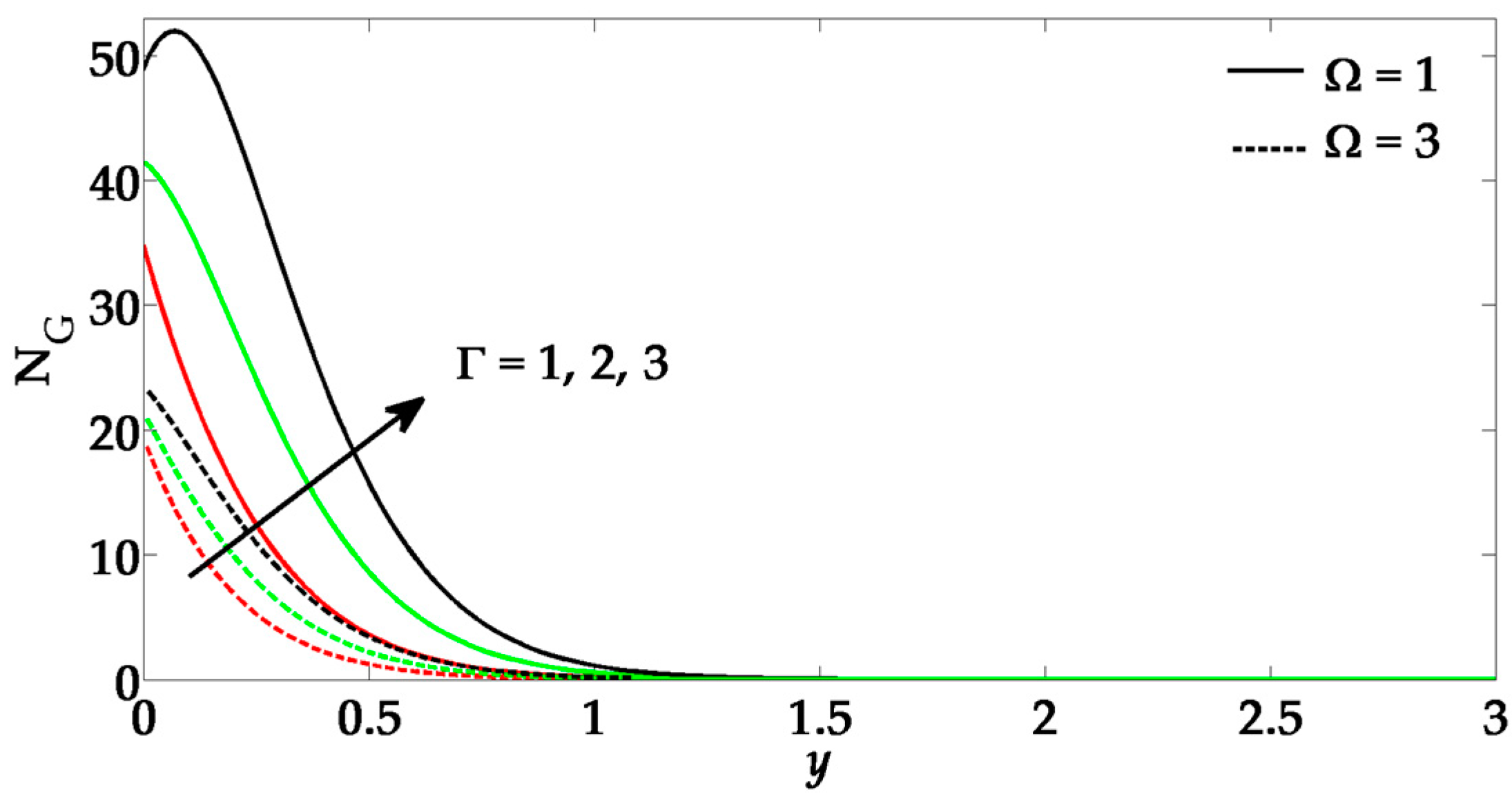
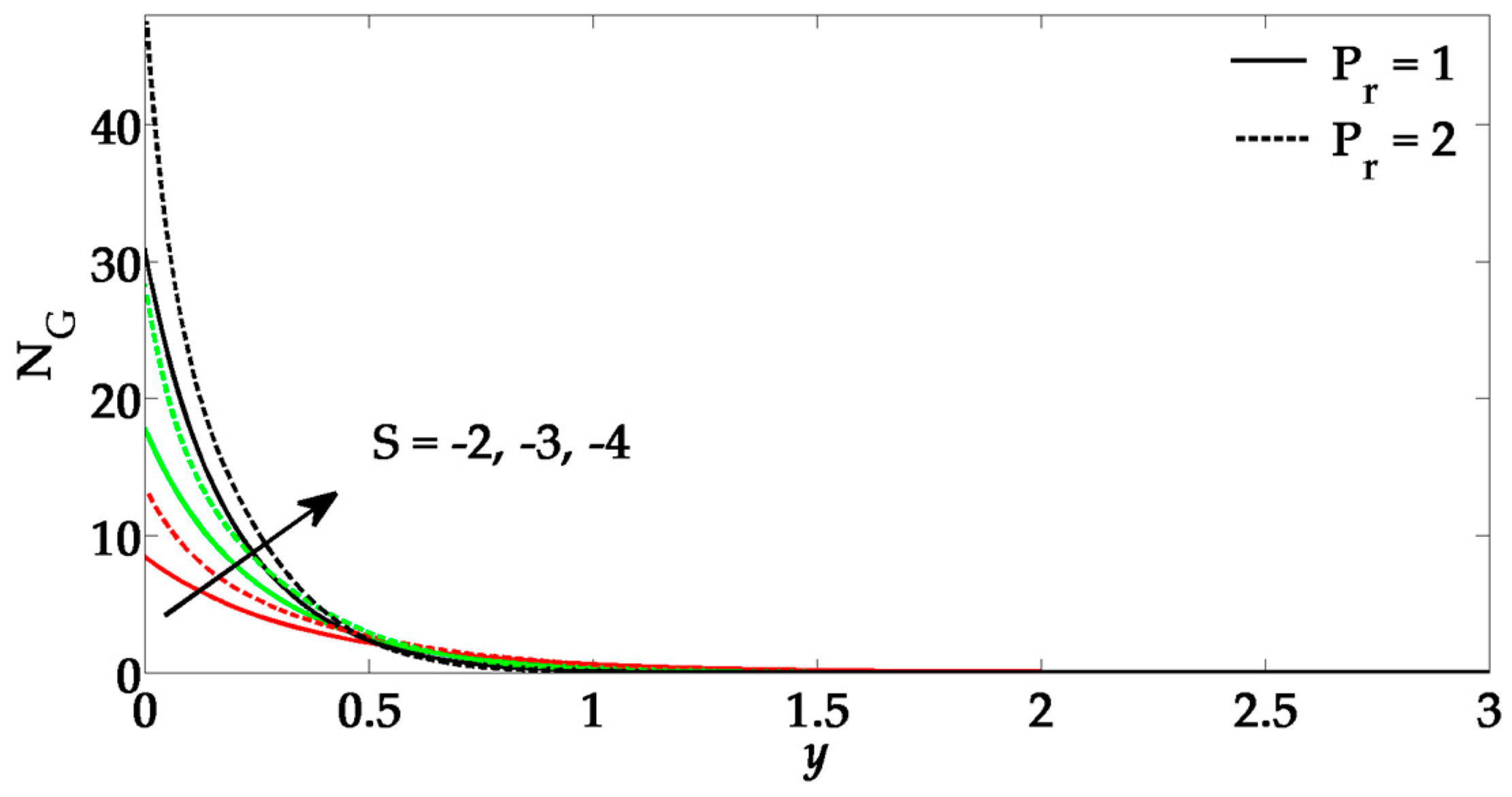
The entropy profile behaves as an increasing function of all the pertinent parameters.

References

1. Ahmad, A.; Asghar, S.; Afzal, S. Flow of nanofluid past a Riga plate. J. Magn. Magn. Mater. 2016, 402, 44–48. [Google Scholar] [CrossRef]
2. Kuznetsov, A.V.; Nield, D.A. Natural convective boundary-layer flow of a nanofluid past a vertical plate. Inter. J. Therm. Sci. 2010, 49, 243–247. [Google Scholar] [CrossRef]
3. Sheikholeslami, M.; Ganji, D.D.; Javed, M.Y.; Ellahi, R. Effect of thermal radiation on magnetohydrodynamics nanofluid flow and heat transfer by means of two phase model. J. Magn. Magn. Mater. 2015, 374, 36–43. [Google Scholar] [CrossRef]
4. Sheikholeslami, M.; Ganji, D.D. Heat transfer of Cu-water nanofluid flow between parallel plates. Powder Technol. 2013, 235, 873–879. [Google Scholar] [CrossRef]
5. Zeeshan, A.; Baig, M.; Ellahi, R.; Hayat, T. Flow of viscous nanofluid between the concentric cylinders. J. Comput. Theor. Nanosci. 2014, 11, 646–654. [Google Scholar] [CrossRef]
6. Pantzali, M.N.; Kanaris, A.G.; Antoniadis, K.D.; Mouza, A.A.; Paras, S.V. Effect of nanofluids on the performance of a miniature plate heat exchanger with modulated surface. Int. J. Heat Fluid Flow 2009, 30, 691–699. [Google Scholar] [CrossRef]
7. Sheikholeslami, M.; Ellahi, R. Electrohydrodynamic nanofluid hydrothermal treatment in an enclosure with sinusoidal upper wall. Appl. Sci. 2015, 5, 294–306. [Google Scholar] [CrossRef]
8. Rahman, S.U.; Ellahi, R.; Nadeem, S.; Zia, Q.Z. Simultaneous effects of nanoparticles and slip on Jeffrey fluid through tapered artery with mild stenosis. J. Mol. Liquids 2016, 218, 484–493. [Google Scholar] [CrossRef]
9. Zeeshan, A.; Majeed, A.; Ellahi, R. Effect of magnetic dipole on viscous ferro-fluid past a stretching surface with thermal radiation. J. Mol. Liquids 2016, 215, 549–554. [Google Scholar] [CrossRef]
10. Rashidi, S.; Dehghan, M.; Ellahi, R.; Riaz, M.; Jamal-Abad, M.T. Study of stream wise transverse magnetic fluid flow with heat transfer around an obstacle embedded in a porous medium. J. Magn. Magn. Mater. 2015, 378, 128–137. [Google Scholar] [CrossRef]
11. Sheikholeslami, M.; Ellahi, R. Three dimensional mesoscopic simulation of magnetic field effect on natural convection of nanofluid. Int. J. Heat Mass Tran. 2015, 89, 799–808. [Google Scholar] [CrossRef]
12. Ellahi, R.; Hassan, M.; Zeeshan, A. Study of natural convection MHD nanofluid by means of single and multi-walled carbon nanotubes suspended in a salt-water solution. IEEE Trans. Nanotechnol. 2015, 14, 726–734. [Google Scholar] [CrossRef]
13. Kandelousi, M.S.; Ellahi, R. Simulation of ferrofluid flow for magnetic drug targeting using the Lattice Boltzmann method. Z. Naturforsch. A Phys. 2015, 70, 115–124. [Google Scholar] [CrossRef]
14. Akbar, N.S.; Raza, M.; Ellahi, R. Influence of induced magnetic field and heat flux with the suspension of carbon nanotubes for the peristaltic flow in a permeable channel. J. Magn. Magn. Mater. 2015, 381, 405–415. [Google Scholar] [CrossRef]
15. Ellahi, R.; Aziz, S.; Zeeshan, A. Non-Newtonian nanofluid flow through a porous medium between two coaxial cylinders with heat transfer and variable viscosity. J. Porous Media 2013, 16, 205–216. [Google Scholar] [CrossRef]
16. Ellahi, R.; Hassan, M.; Zeeshan, A. Shape effects of nanosize particles in Cu-H2O nanofluid on entropy generation. Int. J. Heat Mass Tran. 2015, 81, 449–456. [Google Scholar] [CrossRef]
17. Zeeshan, A.; Majeed, A. Non Darcy Mixed Convection Flow of Magnetic Fluid over a Permeable Stretching Sheet with Ohmic Dissipation. J. Magn. 2016, 21, 153–158. [Google Scholar] [CrossRef]
18. Rashidi, M.M.; Abelman, S.; Mehr, N.F. Entropy generation in steady MHD flow due to a rotating porous disk in a nanofluid. Int. J. Heat Mass Tran. 2013, 62, 515–525. [Google Scholar] [CrossRef]
19. Nawaz, M.; Zeeshan, A.; Ellahi, R.; Abbasbandy, S.; Rashidi, S. Joules and Newtonian heating effects on stagnation point flow over a stretching surface by means of genetic algorithm and Nelder-Mead method. Int. J. Numer. Method Heat Fluid Flow 2015, 25, 665–684. [Google Scholar] [CrossRef]
20. Abolbashari, M.H.; Freidoonimehr, N.; Nazari, F.; Rashidi, M.M. Entropy analysis for an unsteady MHD flow past a stretching permeable surface in nano-fluid. Powder Technol. 2014, 267, 256–267. [Google Scholar] [CrossRef]
21. Abolbashari, M.H.; Freidoonimehr, N.; Nazari, F.; Rashidi, M.M. Analytical modeling of entropy generation for Casson nano-fluid flow induced by a stretching surface. Adv. Powder Technol. 2015, 26, 542–552. [Google Scholar] [CrossRef]
22. Qing, J.; Bhatti, M.M.; Abbas, M.A.; Rashidi, M.M.; Ali, M.E.S. Entropy Generation on MHD Casson Nanofluid Flow over a Porous Stretching/Shrinking Surface. Entropy 2016, 18. [Google Scholar] [CrossRef]
23. Bhatti, M.M.; Rashidi, M.M. Effects of thermo-diffusion and thermal radiation on Williamson nanofluid over a porous shrinking/stretching sheet. J. Mol. Liquids 2016. [Google Scholar] [CrossRef]
24. Zeeshan, A.; Hassan, M.; Ellahi, R.; Nawaz, M. Shape effect of nanosize particles in unsteady mixed convection flow of nanofluid over disk with entropy generation. J. Process Mech. Eng. 2016. [Google Scholar] [CrossRef]
25. Bhatti, M.M.; Abbas, T.; Rashidi, M.M.; Ali, M.E.S. Numerical simulation of entropy generation with thermal radiation on MHD Carreau nanofluid towards a shrinking sheet. Entropy 2016, 18. [Google Scholar] [CrossRef]
Figure 1. Geometry of the problem.
Entropy 18 00223 g001
Figure 2. Velocity profile for different values of λ and N R   when P r = 1 ,   N b = N t = 0.2 ,   L e = 1 . Solid red line:   N R = 0.5 ,   λ = 1 ; Dashed red line:   N R = 2 ,   λ = 1 ; Solid green line:   N R = 0.5 ,   λ = 2 ; Dashed green line:   N R = 2 ,   λ = 2 ; Solid black line:   N R = 0.5 ,   λ = 3 ; Dashed black line:   N R = 2 ,   λ = 3 .
Entropy 18 00223 g002
Figure 3. Velocity profile for different values of S and P r when N R = 0.5 ,   λ = 1 ,   N b = N t = 0.2 ,   L e = 1 . Solid red line: P r = 1 ,   S = 2 ; Dashed red line: P r = 2 ,   S = 2 ; Solid green line: P r = 1 ,   S = 3 ; Dashed green line: P r = 2 ,   S = 3 ; Solid black line: P r = 1 ,   S = 4 ; Dashed black line: P r = 2 ,   S = 4 .
Entropy 18 00223 g003
Figure 4. Temperature profile for different values of N t and S when P r = 1 ,   N R = 0.5 ,   λ = 1 ,   N b = 0.2 ,   L e = 1 . Solid red line:   N t = 0.2 ,   S = 3 ; Dashed red line:   N t = 0.2 ,   S = 4 ; Solid green line:   N t = 0.4 ,   S = 3 ; Dashed green line:   N t = 0.4 ,   S = 4 ; Solid black line:   N t = 0.6 ,   S = 3 ; Dashed black line:   N t = 0.6 ,   S = 4 .
Entropy 18 00223 g004
Figure 5. Temperature profile for different values of N b and P r when N R = 0.5 ,   λ = 1 ,   N t = 0.2 ,   L e = 1 . Solid red line:   N b = 0.2 ,   P r = 1 ; Dashed red line:   N b = 0.2 ,   P r = 2 ; Solid green line:   N b = 0.4 ,   P r = 1 ; Dashed green line:   N b = 0.4 ,   P r = 2 ; Solid black line:   N b = 0.6 ,   P r = 1 ; Dashed black line:   N b = 0.6 ,   P r = 2 .
Entropy 18 00223 g005
Figure 6. Concentration profile for different values of L e and S when P r = 1 ,   N R = 0.5 ,   λ = 1 ,   N b = N t = 0.2 . Solid red line:   L e = 1 ,   S = 3 ; Dashed red line:   L e = 1 ,   S = 4 ; Solid green line:   L e = 2 ,   S = 3 ; Dashed green line:   L e = 2 ,   S = 4 ; Solid black line:   L e = 3 ,   S = 4 ; Dashed black line:   L e = 3 ,   S = 4 .
Entropy 18 00223 g006
Figure 7. Concentration profile for different values of N b   and P r when N R = 0.5 ,   λ = 1 ,   N t = 0.2 ,   L e = 1 . Solid red line:   N b = 0.2 ,   P r = 1 ; Dashed red line:   N b = 0.2 ,   P r = 2 ; Solid green line:   N b = 0.4 ,   P r = 1 ; Dashed green line:   N b = 0.4 ,   P r = 2 ; Solid black line:   N b = 0.6 ,   P r = 1 ; Dashed black line:   N b = 0.6 ,   P r = 2 .
Entropy 18 00223 g007
Figure 8. Concentration profile for different values of N t and S   when P r = 1 ,   N R = 0.5 ,   λ = 1 ,   N b = 0.2 ,   L e = 1 . Solid red line:   N t = 0.2 ,   S = 3 ; Dashed red line:   N t = 0.2 ,   S = 4 ; Solid green line:   N t = 0.4 ,   S = 3 ; Dashed green line:   N t = 0.4 ,   S = 4 ; Solid black line:   N t = 0.6 ,   S = 3 ; Dashed black line:   N t = 0.6 ,   S = 4 .
Entropy 18 00223 g008
Figure 9. Entropy profile for different values of B r and ζ when P r = 1 ,   N R = 0.5 ,   λ = 1 ,   N b = N t = 0.2 ,   L e = 1 . Solid Red Line: ζ = 1 ,   B r = 1 ; Dashed Red Line: ζ = 3 ,   B r = 1 ; Solid green line: ζ = 1 ,   B r = 2 ; Dashed green line: ζ = 3 ,   B r = 2 ; Solid black line: ζ = 3 ,   B r = 3 ; Dashed black line: ζ = 3 ,   B r = 3 .
Entropy 18 00223 g009
Figure 10. Entropy profile for different values of Γ   and Ω when P r = 1 ,   N R = 0.5 ,   λ = 1 ,   N b = N t = 0.2 ,   L e = 1 . Solid Red Line: Γ = 1 ,   Ω = 1 ; Dashed Red Line: Γ = 1 ,   Ω = 3 ; Solid green line: Γ = 2 ,   Ω = 1 ; Dashed green line: Γ = 2 ,   Ω = 3 ; Solid black line: Γ = 3 ,   Ω = 1 ; Dashed black line: Γ = 3 ,   Ω =   3 .
Entropy 18 00223 g010
Figure 11. Entropy profile for different values of S and P r when N R = 0.5 ,   λ = 1 ,   N b = N t = 0.2 ,   L e = 1 . Solid red line: P r = 1 ,   S = 2 ; Dashed red line: P r = 2 ,   S = 2 ; Solid green line: P r = 1 ,   S = 3 ; Dashed green line: P r = 2 ,   S = 3 ; Solid black line: P r = 1 ,   S = 4 ; Dashed black line: P r = 2 ,   S = 4 .
Entropy 18 00223 g011