Extreme Learning Machine for Multi-Label Classification

Abstract

Extreme learning machine (ELM) techniques have received considerable attention in the computational intelligence and machine learning communities because of the significantly low computational time required for training new classifiers. ELM provides solutions for regression, clustering, binary classification, multiclass classifications and so on, but not for multi-label learning. Multi-label learning deals with objects having multiple labels simultaneously, which widely exist in real-world applications. Therefore, a thresholding method-based ELM is proposed in this paper to adapt ELM to multi-label classification, called extreme learning machine for multi-label classification (ELM-ML). ELM-ML outperforms other multi-label classification methods in several standard data sets in most cases, especially for applications which only have a small labeled data set.

1. Introduction

Multi-label classification deals with one object which possibly belongs to multiple labels simultaneously, which are common in real-world applications, such as text categorization, scene and video annotation, bioinformatics, and music emotion classification [1]. For example, a sunrise image could be labeled with “sun,” “sky” and “sea” at the same time in semantic scene classification. Formally [2], let $\mathcal{X}={ℝ}^{\mathrm{d}}$ denote the d-dimensional input space, and $\mathcal{Y}=\left\{y_1,y_2,\dots ,y_m\right\}$ denote the label space consisting of m possible class labels. The task of multi-label learning is to learn a function: $\mathrm{h}:\mathcal{X}\to 2^{\mathcal{Y}}$ from the multi-label training set $\mathcal{D}=\left\{\left(x_i,Y_i\right)|1\le i\le n\right\}.$ For each multi-label example ($x_i,Y_i$), $x_i\in \mathcal{X}$ is a d-dimensional feature vector ($x_{i1},x_{i2},\dots ,x_{id}$) T and $Y_i\subseteq \mathcal{Y}$ is the relevant label with $x_i$. For any unseen instance $x_i\in \mathcal{X}$, the multi-label classifier $h(·)$ predicts $h\left(x\right)\subseteq \mathcal{Y}$ as the set of proper labels for $x$.

Multi-label classification has attracted a lot of attention in the past few years [3,4,5,6]. Nowadays, there are two main ways to construct various discriminative multi-label classification algorithms: problem transformation and algorithm adaptation. The key philosophy of problem transformation methods is to fit the data to the algorithm, while the key philosophy of algorithm adaptation methods is to fit the algorithm to the data [2].

A problem transformation strategy tackles a multi-label learning problem by transforming it into multiple independent binary or multi-class sub-problems, constructing a sub-classifier for each sub-problem using an existing technique, and then assembling all sub-classifiers into an entire multi-label classifier. It is convenient and fast to implement a problem transformation method due to the number of existing techniques and their free software. Representative algorithms include Binary Relevance [7], AdaBoost.MH [8], Calibrated Label Ranking [3], Random k-labelsets [9], etc.

An algorithm adaptation strategy tackles multi-label learning problem by adapting popular learning techniques to deal with multi-label data. Representative algorithms include Multi-Label k-Nearest Neighbor (ML-kNN) [10], Multi-Label Decision Tree (ML-DT) [11], Ranking Support Vector Machine (Rank-SVM) [12], Backpropagation for Multi-Label Learning (BP-MLL) [13], etc. The basic idea of ML-kNN is to adapt k-nearest neighbor techniques to deal with multi-label data, where a maximum a posteriori (MAP) rule is utilized to make predictions by reasoning with the labeling information embodied in the neighbors. The basic idea of BP-MLL is to adapt feed-forward neural networks to deal with multi-label data, where the error back propagation strategy is employed to minimize a global error function capturing label correlations.

In the multi-labeled setting, classes belonging to one instance are often related to each other. The performance of the multi-label learning system is poor if it ignores the relationships between the different labels of each instance. Therefore, the famous Rank-SVM defines the margin over hyper planes for relevant–irrelevant label pairs, which explicitly characterizes label correlations of an individual instance. Rank-SVM achieves great accuracy. Unfortunately, Rank-SVM has a high computational cost, which limits its usability for many applications. Therefore, it is still necessary to build some novel efficient multi-label algorithms.

Recently, Huang et al. [14,15,16] proposed a novel learning algorithm for single-hidden layer feedforward neural networks called extreme learning machine (ELM). The single-hidden layer feedforward neural networks have been widely applied in machine learning [17,18,19,20,21,22] and ELM represents one of the recent successful approaches in machine learning. Compared with traditional computational intelligence techniques, ELM exhibits better generalization performance at a much faster learning speed and with fewer human interventions. ELM techniques have received considerable attention in computational intelligence and machine learning communities, in both theoretic study and applications [23,24,25,26,27,28,29]. ELM provides solutions to regression, clustering, feature learning, binary classification and multiclass classifications, but not to multi-label learning, which is a harder task than traditional binary and multi-class problems. Therefore, a thresholding method-based ELM is proposed in this paper to adapt ELM to multi-label classification, called ELM-ML (Extreme Learning Machine for Multi-Label classification). Experiments on eight multi-label datasets show that the performance of ELM-ML is superior to some other well-established multi-label learning algorithms including Rank-SVM, ML-kNN, BP-MLL and Multi-Label Naïve Bayes (MLNB) in most cases, especially for applications which only have a small labeled data set.

2. A Brief Review of ELM

This section briefly reviews the standard ELM [14]. ELM was originally proposed for single hidden-layer feedforward neural networks (SLFNs). For N arbitrary distinct samples ($x_i,t_i$), where $x_i={\left[x_{i1},x_{i2},\dots ,x_{id}\right]}^T\in {\mathrm{R}}^{\mathrm{d}}$ and $t_i={\left[t_{i1},t_{i2},\dots ,t_{im}\right]}^T\in {\mathrm{R}}^{\mathrm{m}}$, standard SLFNs with $\tilde{N}$ hidden nodes and activation function $\mathrm{g}\left(\mathrm{x}\right)$ are mathematically modeled as

$${\displaystyle \sum }_{i=1}^{\tilde{N}}{\beta }_{i}g\left(x_j\right)={\displaystyle \sum }_{i=1}^{\tilde{N}}{\beta }_{i}g\left(w_i·x_j+b_i\right)=o_j, j=1,\dots ,N$$

(1)

where $w_i={\left[w_{i1},w_{i2},\dots ,w_{iN}\right]}^T$ is the weight vector connecting the ith hidden node and the input nodes, ${\beta }_i={\left[{\beta }_{i1},{\beta }_{i2},\dots ,{\beta }_{im}\right]}^T$ is the weight vector connecting the ith hidden node and the output nodes, and $b_i$ is the thresholding of the ith hidden node. $w_i·x_j$ denotes the inner product of $w_i$ and $x_j$. If a SLFNs with $\tilde{N}$ hidden nodes with activation function $g\left(x\right)$ can approximate these N samples with zero error, it means that ${\displaystyle \sum }_{j=1}^{\tilde{N}}\parallel o_j-t_j\parallel =0$, i.e., there exist ${\beta }_i$, $w_i$ and $b_i$ such that

$${{\displaystyle \sum }}_{i=1}^{\tilde{N}}{\beta }_{i}g\left(w_i·x_j+b_i\right)=t_j, j=1,\dots ,N$$

(2)

The above N equations can be written compactly as

$$H\beta =T$$

(3)

where

$$H=\left[\begin{array}{c}h\left(x_1\right)\\ ⋮\\ h\left(x_N\right)\end{array}\right]={\left[\begin{array}{ccc}g\left(w_1·x_1+b_1\right)& \cdots & g\left(w_{\tilde{N}}·x_1+b_{\tilde{N}}\right)\\ ⋮& \ddots & ⋮\\ g\left(w_1·x_N+b_1\right)& \cdots & g\left(w_{\tilde{N}}·x_N+b_{\tilde{N}}\right)\end{array}\right]}_{N\times \tilde{N}}$$

(4)

$$\beta ={\left[\begin{array}{c}{\beta }_1^T\\ ⋮\\ {\beta }_{\tilde{N}}^T\end{array}\right]}_{\tilde{N}\times m}\mathrm{and} T={\left[\begin{array}{c}{t}_1^T\\ ⋮\\ t_N^T\end{array}\right]}_{N\times m}$$

(5)

H is called the hidden layer output matrix of the SLFN; the ith column of H is the ith hidden node output with respect to inputs $x_1$, $x_2$,…, $x_N$. It has been proven [15] that if the activation function g is infinitely differentiable in any interval, the hidden layer parameters can be randomly generated. Therefore, Formula (3) becomes a linear system and the output weights $\beta$ are estimated as

$$\widehat{\beta }= H^{†}T,$$

(6)

where $H^{†}$ is the Moore–Penrose generalized inverse of the hidden layer output matrix H. Thus, ELM randomly generated hidden node parameters and then analytically calculated the hidden layer output matrix H and the output weights $\beta$. This avoids any long training procedure where a hidden layer of SLFNs need to be tuned. Compared with traditional computational intelligence techniques, ELM provides better generalization performance at a much faster learning speed and with fewer human interventions.

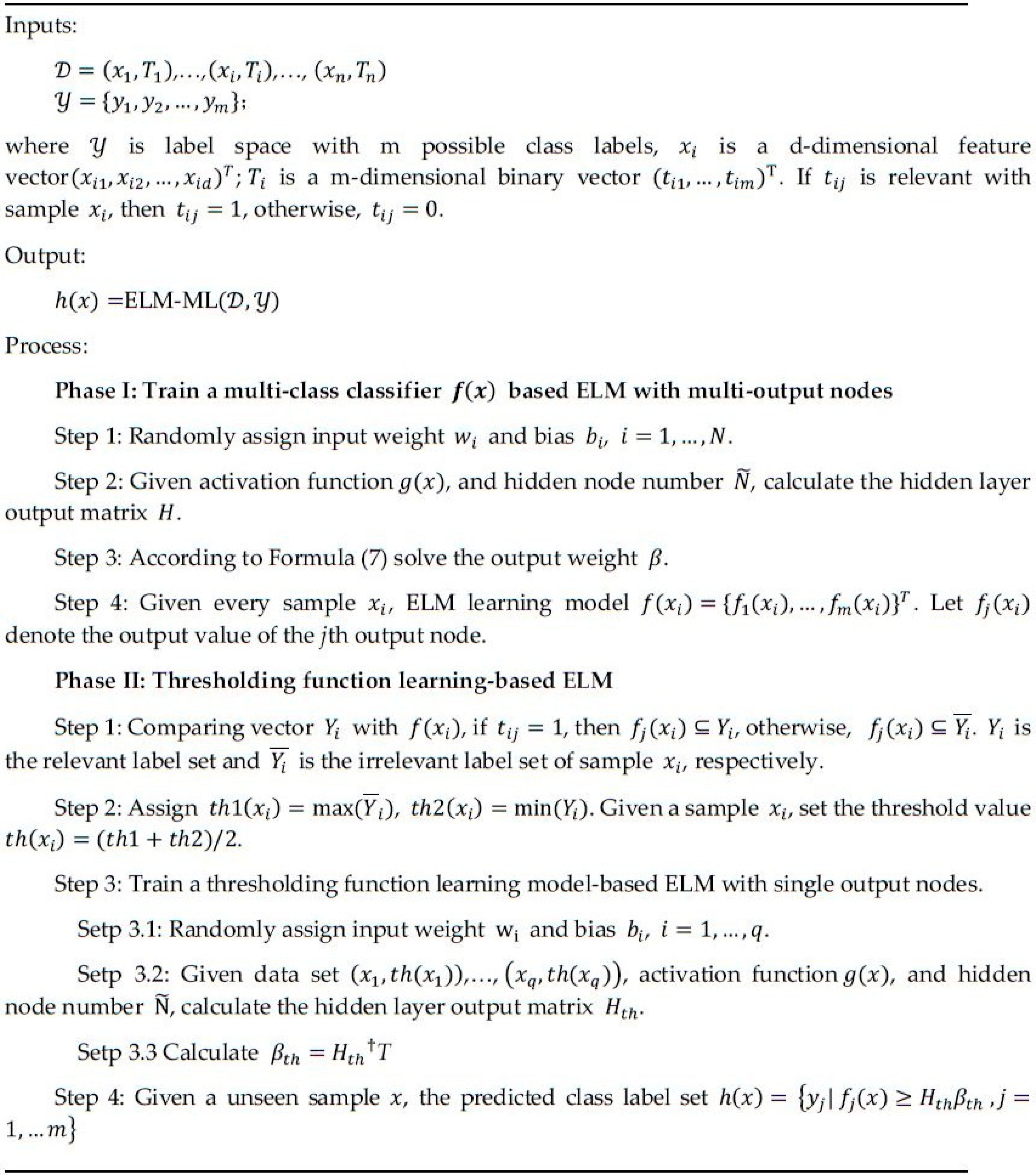
3. ELM-ML

In this section, we will describe our multi-label classification algorithm, called an extreme learning machine for multi-label classification (ELM-ML).

From the standard optimization method point of view [15], ELM with multi-output nodes can be formulated as

$$\mathrm{Minimize}: \frac{1}{2}{\parallel \beta \parallel }^2+C\frac{1}{2}{{\displaystyle \sum }}_{i=1}^N\parallel {\xi }_i\parallel {}^2, \mathrm{Subject\; to} h\left(x_i\right)\beta =t_i^T-{\xi }_i^T$$

(7)

Formula (7) tends to reach not only the smallest training error but also the smallest norm of output weights, where $1\le i\le N$. N is the number of training samples. ${\xi }_i= {\left[{\xi }_{i,1},\dots ,{\xi }_{i,m}\right]}^T$ is the training error vector of the m output nodes with respect to the training sample $x_i$. C is a user-specified parameter and provides a trade-off between the distance of the separating margin and the training error. The predicted class label of a given testing sample is the index number of the output node which has the highest output value. Formula (7) provides a solution to multi-class classifications.

Multi-label learning is a harder task than traditional multi-class problems, which is a special case of multi-label classification. One sample belongs to several related labels simultaneously, so we cannot simply regard the index number of the highest output value as a predicted class for a given testing sample. A proper thresholding function $th\left(x\right)$ should be set. Naturally, the predicted class labels for a given testing sample are those index numbers for output nodes which have higher output value than the predefined thresholding.

Setting $th\left(x\right)$ as a constant function is a common multi-label thresholding method. One straightforward choice is to use zero as the calibration constant [7,8]. An alternative choice for the calibration constant is 0.5, when the multi-label learned model $f\left(x,y\right)$ represents the posterior probability of $y$ being a proper label of $x$ [10,11,23]. Another popular approach, called experimental thresholding [30], consists in testing different values as thresholds on a validation set and choosing the value which maximizes the effectiveness. Of all the threshold calibration strategies above, experimental thresholding seems to be the most reasonable, but it is time-consuming and labor-intensive. We believe that the thresholding function $th\left(x\right)$ should be learned from instances. That is to say, different instances should correspond to different thresholdings in multi-label learning model. A novel method would be to consider the thresholding function $th\left(x\right)$ as a regression problem for the training data. In this paper, we use an ELM algorithm with a single output node to solve this regression problem. Overall, the proposed ELM-ML algorithm has two phases: multi-class classifier-based ELM with multi-outputs and thresholding function learning-based ELM with single outputs. The pseudo-code of ELM-ML is summarized in Figure 1.

4. Experiments

Firstly, we compare the proposed thresholding strategy in this paper with the constant thresholding strategy and strategy in Rank-SVM [12]. Secondly, we compare the performance of different multi-label classification algorithms, including our algorithm ELM-ML, Rank-SVM, MLNB, BP-MLL [13] and ML-kNN [10] on eight multi-label classification data sets. Before presenting our experimental results, we briefly introduce eight benchmark data sets and six multi-label performance measures.

4.1. Datasets

In order to verify the performance of thresholding strategy and different multi-label classification algorithms, a wide variey of data sets have been tested in our simulations, which are of small/large sizes, low/high dimensions, and small/large labels. These data sets [31] include diversified multi-label classification cases, which cover four distinct domains: text, scene, music and biology.

To characterize the properties of the multi-label data sets, several useful multi-label indicators can be utilized. The most natural way to measure the degree of multi-labeledness is Label Cardinality (LC): $LC\left(\mathcal{D}\right)=\frac{1}{m}{\displaystyle \sum }_{i=1}^m|Y_i|$, i.e., the average number of labels per sample. Accordingly, Label Density(LD) normalizes label cardinality by the number of possible labels in the label space: $LD\left(\mathcal{D}\right)=\frac{1}{|y|}·LC\left(\mathcal{D}\right)$.

Table 1. Information for eight benchmark data sets.

Dataset	Domain	#Training	#Test	Attributes	Labels	LC	LD
Small data sets
Genbase	Biology	463	191	1185	27	1.35	0.050
Emotions	Music	391	202	72	6	1.87	0.312
CAL500	Music	300	202	68	174	26.04	0.150
Medium data sets
Yeast	Biology	1500	917	103	14	4.24	0.303
Scene	Scene	1211	1196	294	6	1.07	0.178
Enron	Text	1123	579	1001	53	3.38	0.064
Large data sets
TMC2007-500	Text	21519	7077	500	22	2.16	0.098
TMC2007	Text	21519	7077	49060	22	2.16	0.098

describes these eight benchmark data sets, in which #Training and #Test means the numbers of training examples and test examples, respectively. As shown in Table 1, the data sets cover a different range of cases whose characteristics are diversified. These data sets are categorized into three groups, such as small data sets, medium data sets and large data sets, according to the amount of training samples. Significantly, there are not only low or high dimensions but also small or large labels in any group.

4.2. Evaluation Measures

With the aim of fair and honest evaluation, performance of the multi-label learning algorithms should be tested on a broad range of metrics instead of only on the one being optimized. In this paper, we chose six evaluation criteria suitable for classification: Subset Accuracy, Hamming Loss, Accuracy, Precision, Recall and F1. These measures are defined as follows [2].

Assume a test data set of size n to be S = {($x_1,Y_1$),…, ($x_i,Y_i$),…, ($x_n,Y_n$)} and $h(·)$ be the learned multi-label classifier. A common practice in multi-label learning is to return a real-valued function $f\left(x,y\right)$. For a unseen instance $x$, the real-valued output $f\left(x,y\right)$ on each label should be calibrated against the thresholding function output $th\left(x\right)$.

• Hamming Loss

The hamming loss evaluates the fraction of misclassified instance-label pairs, i.e., a relevant label is missed or an irrelevant label is predicted.

$$\text{Hamming Loss}\left(h\right)=\frac{1}{n}{\displaystyle \sum }_{i=1}^n|h\left(x_i\right)\Delta Y_i|$$

(8)

where $\Delta$ stands for the symmetric difference between two sets.

• Subset Accuracy

The subset accuracy evaluates the fraction of correctly classified examples, i.e., the predicted label set is identical to the ground-truth label set. Intuitively, subset accuracy can be regarded as a multi-label counterpart of the traditional accuracy metric, and tends to be overly strict especially when the size of the label space is large.

$$\text{Subset Accuracy}\left(h\right)=\frac{1}{n}{\displaystyle \sum }_{i=1}^n|h\left(x_i\right)=Y_i|$$

(9)

• Accuracy, Precision, Recall and F1

$$\text{Accuracy}\left(h\right)=\frac{1}{n}{\displaystyle \sum }_{i=1}^n\frac{|Y_i{{\displaystyle \cap }}^{\text{}}h\left(x_i\right)|}{|Y_i{{\displaystyle \cup }}^{\text{}}h\left(x_i\right)|}$$

(10)

$$\text{Precison}\left(h\right)=\frac{1}{n}{\displaystyle \sum }_{i=1}^n\frac{|Y_i{{\displaystyle \cap }}^{\text{}}h\left(x_i\right)|}{|h\left(x_i\right)|}$$

(11)

$$\text{Recall}\left(h\right)=\frac{1}{n}{\displaystyle \sum }_{i=1}^n\frac{|Y_i{{\displaystyle \cap }}^{\text{}}h\left(x_i\right)|}{|Y_i|}$$

(12)

$$\mathrm{F}1\left(h\right)=\frac{2\times \text{Precision}\left(h\right)\times \text{Recall}\left(h\right)}{\text{Precision}\left(h\right)+\text{Recall}\left(h\right)}$$

(13)

Here, $Y_i$ and $h\left(x_i\right)$ correspond to the ground-truth and predicted label set for $x_i$, respectively.

Obviously, except for the first metrics, the larger the last five metric value, the better the system’s performance is.

4.3. Results

4.3.1. Thresholding Function

We compare three thresholding strategies: the proposed thresholding strategy in ELM-ML, thresholding strategy in Rank-SVM and constant strategy. To achieve an optimal constant thresholding parameter Ct, we tested different values as thresholdings on the validation set and chose the value which maximizes the effectiveness. More specifically, hamming loss and subset accuracy are regarded as criteria to tune constant parameter Ct, respectively. Constant parameter Ct is tuned from −1 to 1 with interval step rate $\delta =0.1$. Rank-SVM employs the stacking-style procedure to set the thresholding function $th\left(x\right)$ [12]. We apply multi-class ELM algorithm providing scores for each sample, then use three thresholding strategies, called ELM-ML, ELM-Rank-SVM and ELM-Constant, to predict labels for each sample.

In experiments, our computational platform is a 32-bit HP workstation with Interl^® (Santa Clara, CA, USA) Core^TM i3-2130 CPU (4CPUs) except for on TMC2007-500 data set and TMC2007 data set, because the amount of training data for these two data sets is very large, and for which the computational platform is a 64-bit HP server with Interl^® Core^TM i7-4700MQ CPU (8CPUs).

All results are detailed in

Table 2. Hamming loss for three thresholding strategies on eight data sets (hamming loss ↓).

Datasets	Algorithms
	ELM-ML	ELM-Rank-SVM	ELM-Constant
Small data sets
Genbase	9.3058 × 10−4	0.9544	0.0013 (Ct = −0.6)
Emotions	0.2087	0.2145	0.2129 (Ct = −0.2)
CAL500	0.1621	0.1837	0.1447 (Ct = 0.6)
Medium data sets
Yeast	0.1980	0.2354	0.2052 (Ct = 0.0)
Scene	0.1193	0.1178	0.1506 (Ct = 0.8)
Enron	0.0851	0.9290	0.0598 (Ct = 0.8)
Large data sets
TMC2007-500	0.0537	0.0568	0.0537 (Ct = −0.1)
TMC2007	0.0631	0.0854	0.0632 (Ct = −0.1)

,

Table 3. Subset sccuracy for three thresholding strategies on eight data sets (subset accuracy ↑).

Datasets	Algorithms
	ELM-ML	ELM-Rank-SVM	ELM-Constant
Small data sets
Genbase	0.9749	0	0.9648 (Ct = −0.6)
Emotions	0.2673	0.2426	0.2574 (Ct = −0.2)
CAL500	0	0	0 (Ct = −1)
Medium data sets
Yeast	0.1919	0.0796	0.1603 (Ct = −0.2)
Scene	0.5042	0.4339	0.5117 (Ct = 0)
Enron	0.0708	0	0.0570 (Ct = 0.4)
Large data sets
TMC2007	0.3290	0.3213	0.3150 (Ct = −0.1)
TMC2007-500	0.2538	0.0308	0.2436 (Ct = −0.1)

and

Table 4. Computation time of non-constant thresholding strategies.

Datasets	ELM-ML		ELM-Rank-SVM
	Training Time (Second)	Testing Time (Second)	Training Time (Second)	Testing Time (Second)
Small data sets
Genbase	1.0739	0.0212	4.6656	0.0673
Emotions	0.5016	0.0064	0.7916	0.0190
CAL500	1.1490	0.0159	14.110	0.2024
Medium data sets
Yeast	0.8094	0.0291	7.3444	0.1197
Scene	1.4300	0.0508	2.4536	0.1110
Enron	3.3922	0.0504	19.6976	0.2460
Large data sets
TMC2007-500	150.83	0.2312	198.72	0.7656
TMC2007	15247	7.3831	22777	8.7663

. The best performance is highlighted in boldface. As seen in Table 2, Table 3 and Table 4, the proposed thresholding strategy in ELM-ML achieves the highest performance among them in most cases. It is worthwhile to note that we tune parameter Ct very carefully on each data set in a constant thresholding strategy. The hamming loss and subset accuracy measures are regarded as criteria to tune parameter Ct. That is to say, when we verified these three thresholding strategies using hamming loss, hamming loss was regarded as a criterion to tune parameter Ct; when we verified these three thresholding strategies using subset accuracy, subset accuracy was regarded as a criterion to tune parameter Ct. Unfortunately, a constant thresholding strategy holds only a slight advantage in the subset accuracy criterion for the scene data set. Meanwhile, the constant thresholding strategy outperforms others for the hamming loss criterion only on the Enron and CAL500 data sets.

Training times and testing times are listed in Table 4. We only compare running time of the thresholding strategy in ELM-ML and the thresholding strategy in Rank-SVM, because the constant thresholding is time-consuming. Obviously, ELM-ML achieves overwhelming performance. In conclusion, the proposed thresholding strategy in ELM-ML is effective and efficient.

4.3.2. Multi-Label Algorithms

We also compare the performances of different multi-label classification algorithms, including ELM-ML, Rank-SVM, BP-MLL, MLNB and ML-kNN on eight multi-label classification data sets. We downloaded Matlab code [32] of BP-MLL, MLNB and ML-kNN . We developed the ELM-ML algorithm in Matlab and chose a sigmoid activation function. Hidden nodes were set to $\tilde{N}$ = 1000. We accept their recommended parameter settings. The best parameters of BP-MLL, MLNB and ML-kNN reported in the literature [10,13,33], were used. For BP-MLL, the learning rate is fixed at 0.05, the number of hidden neurons is 20% of the number of input neurons, the training epochs is set to be 100 and the regularization constant is fixed to be 0.1. For MLNB, the fraction of remaining features after PCA is set to the moderate value of 0.3. For ML-kNN, the Laplacian estimator s = 1 and k = 10 are used. The number of iterations is fixed at 100. For Rank-SVM developed in Matlab, a Gaussian kernel is tested, where kernel parameter $\gamma$ and cost parameter$C$ need to be chosen appropriately for each data set. In our experiments, the Hamming Loss measure is regarded as a criterion to tune two parameters. To achieve an optimal parameter combination ($\gamma , C$), we use a similar tuning procedure as in [9]. The optimal parameters of Rank-SVM on each data set are shown in

Table 5. The optimal $\gamma$ and $C$ values for each data set.

	Data Sets
	Genbase	Emotions	Yeast	Scene	Enron
$\gamma$	−3	−3	$0$	−4	−2
$C$	0.25	0.125	0.125	1	8
Hamming Loss	0.0865	0.3317	0.2330	0.8077	0.0560

. Due to the large size of the label space, Rank-SVM failed to calculate the results on CAL500. On the other hand, Rank-SVM, BP-MLL and MLNB did not output experimental results for TMC2007 and TMC2007-500. The amounts of training data of TMC2007 and TMC2007-500 are huge, which leads to high computational complexity. BP-MLL needs more iteration, which is time-consuming. Therefore, there are no results on these three data sets or parts of them.

The detailed experimental results are shown in

Table 6. Hamming loss for 5 algorithms on eight data sets (hamming loss ↓).

Datasets	Algorithms
	ELM-ML	ML-kNN	BP-MLL	MLNB	Rank-SVM
Small data sets
Genbase	9.3058 × 10−4	0.0043	0.0037	0.0456	0.0865
Emotions	0.2087	0.2104	0.2252	0.3317	0.3317
CAL500	0.1381	0.1393	0.1409	0.1755	-
Medium data sets
Yeast	0.1980	0.1996	0.2084	0.2330	0.2330
Scene	0.1193	0.0989	0.2907	0.2121	0.8077
Enron	0.0851	0.0519	0.0532	0.1339	0.0560
Large data sets
TMC2007-500	0.0537	0.0576	0.0806	0.1663	-
TMC2007	0.0631	0.0652	-	-	-

,

Table 7. Subset accuracy for 5 algorithms on eight data sets (subset accuracy ↑).

Datasets	Algorithms
	ELM-ML	ML-kNN	BP-MLL	MLNB	Rank-SVM
Small data sets
Genbase	0.9749	0.9246	0.9045	0.0000	0.0000
Emotions	0.2673	0.2376	0.2327	0.0854	0.0000
CAL500	0.0000	0.0000	0.0000	0.0000	-
Medium data sets
Yeast	0.1919	0.1592	0.1516	0.0153	0.1680
Scene	0.5042	0.5727	0.1605	0.1630	0.0000
Enron	0.0708	0.0432	0.1002	0.0069	0.0397
Large data sets
TMC2007-500	0.3290	0.3070	0.1850	0.0418	-
TMC2007	0.2538	0.2436	-	-	-

,

Table 8. Precision for five algorithms on eight data sets (precision ↑).

Datasets	Algorithms
	ELM-ML	ML-kNN	BP-MLL	MLNB	Rank-SVM
Small data sets
Genbase	0.9965	0.9799	0.9724	0.0568	0.9875
Emotions	0.8083	0.7907	0.6625	0.5948	0.7005
CAL500	0.457613	0.6040	0.5856	0.4224	-
Medium data sets
Yeast	0.7542	0.7585	0.7505	0.7090	0.7034
Scene	0.8200	0.8512	0.4490	0.6682	0.7967
Enron	0.5762	0.6234	0.6933	0.2217	0.5949
Large data sets
TMC2007-500	0.7637	0.7383	0.6001	0.3726	-
TMC2007	0.6150	0.6088	-	-	-

,

Table 9. Recall for five algorithms on eight data sets (recall ↑).

Datasets	Algorithms
	ELM-ML	ML-kNN	BP-MLL	MLNB	Rank-SVM
Small data sets
Genbase	0.9958	0.9501	0.9761	0.0000	0.9749
Emotions	0.6691	0.5734	0.6370	0.4711	0.6436
CAL500	0.3757	0.2317	0.2717	0.3610	-
Medium data sets
Yeast	0.6378	0.5491	0.6437	0.5599	0.6544
Scene	0.6413	0.6547	0.1681	0.6083	0.6426
Enron	0.5187	0.3364	0.6422	0.5449	0.5664
Large data sets
TMC2007-500	0.7190	0.6722	0.6706	0.6212	-
TMC2007	0.5947	0.5909	-	-	-

,

Table 10. F1 for five algorithms on eight data sets (F1 ↑).

Datasets	Algorithms
	ELM-ML	ML-kNN	BP-MLL	MLNB	Rank-SVM
Small data sets
Genbase	0.9954	0.9648	0.9717	0.0000	0.9774
Emotions	0.6813	0.6126	0.6483	0.5265	0.6685
CAL500	0.4127	0.3350	0.3712	0.3893	-
Medium data sets
Yeast	0.6683	0.6276	0.6560	0.6205	0.6637
Scene	0.6160	0.6576	0.1701	0.5882	0.6400
Enron	0.4660	0.4241	0.6141	0.3853	0.5608
Large data sets
TMC2007-500	0.7407	0.7037	0.6334	0.4658	-
TMC2007	0.6096	0.6072	-	-	-

,

Table 11. Accuracy for five algorithms on eight data sets (accuracy ↑).

Datasets	Algorithms
	ELM-ML	ML-kNN	BP-MLL	MLNB	Rank-SVM
Small data sets
Genbase	0.9908	0.9502	0.9535	0.0000	0.9749
Emotions	0.5245	0.5008	0.5266	0.4278	0.5552
CAL500	0.2595	0.2004	0.2252	0.2368	-
Medium data sets
Yeast	0.5265	0.4920	0.5184	0.4802	0.5349
Scene	0.5686	0.6293	0.1674	0.5447	0.6106
Enron	0.3195	0.2988	0.4712	0.2145	0.0004
Large data sets
TMC2007-500	0.6127	0.5789	0.4921	0.2986	-
TMC2007	0.4877	0.4869	-	-	-

and

Table 12. Computation time of four algorithms.

	ELM-ML		ML-kNN		BP-MLL		MLNB
	Train (s)	Test (s)	Train (s)	Test (s)	Train (s)	Test (s)	Train (s)	Test (s)
Genbase	1.074	0.021	0.209	0.306	1.013 × 104	5.949	1.466 × 103	0.604
Emotions	0.502	0.006	0.131	0.158	2.606 × 103	1.625	2.408 × 102	0.122
CAL500	1.149	0.016	0.083	0.067	9.561	0.159	0.125	0.160
Yeast	0.809	0.029	0.417	1.358	9.805 × 103	7.684	1.821 × 103	1.064
Scene	1.430	0.050	1.533	0.878	9.243 × 103	2.840	6.561 × 102	0.623
Enron	3.392	0.050	0.461	1.511	2.09 × 104	22.51	3.621 × 103	1.739
TMC2007-500	1.740	0.231	5.113	159.3	6.89 × 102	77.90	1.508 × 102	1.437
TMC2007	1.524 × 104	7.383	6.856 × 103	1.905 × 102	-	-	-	-

. The best performance among the five comparing algorithms is highlighted in boldface. From Table 6, Table 7, Table 8, Table 9, Table 10 and Table 11, ELM-ML obtains the best performances in all six criteria on a small data set. Genbase, Emotions and CAL500 are all small-size training data regardless of the size of labels and feature dimensions. That is to say, the proposed ELM-ML is more suitable to solve those applications for which a large amount of labeled data is difficult to obtain. ELM-ML tends to achieve better results than other well-established multi-label algorithms when only a small amount of labeled training data is available. However, ELM-ML is inferior to others on medium data sets, whereas Rank-SVM and ML-kNN work well. It is interesting that if a large number of labeled data are obtained easily, ELM-ML presents the best performance.

Furthermore, training times and testing times are listed in Table 12. ELM-ML achieves the best testing time and ML-kNN obtains the best training time except on the Scene and TMC2007-500 data sets.

5. Conclusions

In this paper, we present an ELM-ML algorithm to solve multi-label classification. ELM is regarded as a recent successful approach to machine learning, because ELM requires a significantly lower computational time for training a learning model and provides better generalization performance with less human intervention. However, ELM does not provide a solution to multi-label classifications. A post-processing step, threshold calibration strategies, should be used to predict the label set of a given sample. A novel method would be to consider the thresholding function $th\left(x\right)$ as a regression problem for training data with class labels. In this paper, we first use an ELM algorithm with multi-output nodes to train a learning model returning a real-valued function, then use the ELM algorithm with a single output node to learn a thresholding function. Experiments on eight diverse benchmark multi-label datasets show that ELM-ML is effective and efficient.