Fractional-Order Grey Prediction Method for Non-Equidistant Sequences

Abstract

There are lots of non-equidistant sequences in actual applications due to random sampling, imperfect sensors, event-triggered phenomena, and so on. A new grey prediction method for non-equidistant sequences (r-NGM(1,1)) is proposed based on the basic grey model and the developed fractional-order non-equidistant accumulated generating operation (r-NAGO), and the accumulated order is extended from the positive to the negative. The whole r-NAGO deletes the randomness of original sequences in the form of weighted accumulation and improves the exponential law of accumulated sequences. Furthermore, the Levenberg–Marquardt algorithm is used to optimize the fractional order. The optimal r-NGM(1,1) can enhance the predicting performance of the non-equidistant sequences. Results of three practical cases in engineering applications demonstrate that the proposed r-NGM(1,1) provides the significant predicting performance compared with the traditional grey model.

1. Introduction

Non-equidistant sequences, whose sampling times are taken to be not equally spaced, exist widely in many applications due to missing data, event-triggered phenomena, imperfect sensors and clocks [1]. Especially, compressive sensing theory and random sampling techniques [2,3] have been developed so that a number of applications use the non-uniform sampling inherently or by choice. It is important to predict the development of processes and systems based on non-equidistant sequences.

Grey prediction method is an effective tool for handling an uncertain system with limited data and partially-known information [4,5]. It has been widely applied to various fields with better predicting accuracy, including natural science, mechanical engineering, and economic fields. NGM(1,1), the non-equidistant grey model with first-order differential equation and a single variable, is the most commonly-used grey prediction model for non-equidistant sequences. In order to improve its predicting accuracy, matrix analysis [6], trend and potency tracking method [7], and the exponential trait [8] were employed to reconstruct background values of NGM(1,1). The reciprocal [9] and class ratio [10] of the original sequence was also modeled with NGM(1,1). The accumulated method [11], Euler formula [12], and Taylor approximation method [13] were used to estimate parameters of NGM(1,1). Moreover, non-equidistant grey Verhulst model [14], non-equidistant DGM(2,1) [15], and non-equidistant grey power model [16] have been proposed for non-equidistant sequences. In the above grey models, original sequences are mostly transformed into accumulated sequences based on the first-order accumulated generating operation (1-AGO). However, these accumulated data do not always follow the grey exponential law completely, so the existing grey model cannot accurately predict for many actual systems.

With the development of fractional calculus, it has been demonstrated that calculus equations with the non-integer/fractional order can describe dynamical behavior of processes and systems with high accuracy and concise models in various fields [17,18,19]. According to the definition of fractional calculus, Wu [20] proposed the fractional-order accumulated generating operation (r-AGO), which extended the first or positive integer-order into the positive fractional one. Various grey models with the fractional order accumulation, such as the fractional-order time-lag grey model [21], reverse accumulative grey model [22], grey discrete power model [23], and non-homogenous discrete grey model [24], were proposed to improve the predicting accuracy in some fields. Mao [25] developed another fractional grey model, which was an extension of the basic grey model in that first-order differential equations were transformed into fractional differential equations. Meng [26] derived the analytical expression of the fractional order reducing generation operator and verified that this operator satisfied the commutative and exponential law. However, these fractional-order grey models are still based on equidistant sequences. More deviations could be yielded if they are used directly to non-equidistant sequences.

A novel fractional-order non-equidistant accumulated generating operation (r-NAGO) is proposed for the non-equidistant sequence in this paper, and the accumulated order is extended to the negative fraction in order to improve the exponential law of the accumulated sequence. Thus, a new grey prediction method (r-NGM(1,1)) is developed based on r-NAGO and the basic grey model GM(1,1) to enhance the predicting accuracy for the non-equidistant sequence. Some practical cases are employed to compare the predicting accuracy of the proposed r-NGM(1,1) with the traditional non-equidistant grey model (NGM(1,1)).

The work procedure is shown as follows. Section 2 reviews the basic theories about r-AGO and NGM(1,1). Then, r-NAGO and r-NGM(1,1) for the non-equidistant sequence is developed in Section 3. Moreover, three practical cases are illustrated to validate the proposed r-NGM(1,1) in Section 4. Section 5 analyzes further its applicability and sampled intervals. Finally, conclusions and future works are presented in Section 6.

2. Basic Theories

A grey system is one in that some information is known and some unknown [4,5]. In actual applications, many systems can be considered as grey systems because there are always some uncertainties. The partially-known information contains a certain governing relation, though it is too complex or chaotic. The main task of grey system theory is to extract the realistic governing relation of the system from the partially known data. The accumulated generating operation usually smoothes the randomness of the original sequence. Then grey model is used to describe the inherent functional relations with differential equations. GM(1,1), a grey model with a first-order differential equation and a single variable, is the most commonly-used grey prediction model. The estimated sequence is calculated by the grey model and the original sequence can be reverted to describe systemic behavior using an inverse accumulated generating operation. Grey system theory has become an effective method to solve uncertainty systems with less sample size and poor information.

2.1. r-AGO

Assuming that $X^{(0)}=\left\{x^{(0)}(1),x^{(0)}(2),\mathrm{...},x^{(0)}(m)\right\}$ is the original nonnegative sequence, when the first-order accumulated generating operation (1-AGO) is applied on $X^{(0)}$, its first-order accumulated sequence $X^{(1)}=\left\{x^{(1)}(1),x^{(1)}(2),\mathrm{...},x^{(1)}(m)\right\}$ could be obtained as:

$$\{\begin{array}{l}{x}^{(1)}(1)=x^{(0)}(1)\hfill \\ x^{(1)}(k)=x^{(1)}(k-1)+x^{(0)}(k)(k=2,3,\mathrm{...}m)\hfill \end{array}$$

(1)

Equation (1) can be expressed with the matrix as:

$$X^{(1)}=X^{(0)}D$$

(2)

where D is the first-order accumulated matrix:

$$D=\left[\begin{array}{cccc}1& 1& \mathrm{...}& 1\\ 0& 1& \mathrm{...}& 1\\ ⋮& ⋮& & \\ 0& 0& \mathrm{...}& 1\end{array}\right]$$

(3)

So the k-th value in $X^{(1)}$ is:

$$x^{(1)}(k)={\displaystyle \sum _{i=1}^k{x}^{(0)}(i)}$$

(4)

The corresponding second-order and M-order accumulated sequences are:

$$X^{(2)}=X^{(1)}D=X^{(0)}{D}^2$$

(5)

$$X^{(M)}=X^{(0)}{D}^M$$

(6)

The M-order accumulated matrix $D^M$ is equal to the M-th power of D when M is the positive integer. Their values in $D^M$ can be written as:

$${(d^M)}_{ik}=\{\begin{array}{ll}1\hfill & (k=i)\hfill \\ \frac{M(M+1)\mathrm{...}(M+k-i-1)}{\left(k-i\right)!}\hfill & (k>i)\hfill \\ 0\hfill & (k<i)\hfill \end{array}$$

(7)

Thus, the k-th accumulated data in $X^{(M)}$ is:

$$x^{(M)}(k)={\displaystyle \sum _{i=1}^k{(d^M)}_{ik}{x}^{(0)}(i)}$$

(8)

Wu [14] extended the positive integer-order accumulated generating operation into any positive fractional one based on the concepts of fractional calculus. Thus, the fractional-order accumulated sequence $X^{(r)}=\left\{x^{(r)}(1),x^{(r)}(2),\mathrm{...},x^{(r)}(m)\right\}$ can be written as:

$$X^{(r)}=X^{(0)}{D}^r$$

(9)

where r is the accumulated order. It can be called as the fractional order when r is set as the fractional number. According to Equation (7), ${(d^r)}_{ik}$ can be obtained as the follows when $k>i$:

$${(d^r)}_{ik}=\frac{r(r+1)\mathrm{...}(r+k-i-1)}{\left(k-i\right)!}$$

(10)

Based on the Gamma function $\Gamma$ [26], ${(d^r)}_{ik}$ can be written as:

$${(d^r)}_{ik}=\frac{\Gamma (r+k-i)}{\Gamma (r)\Gamma \left(k-i+1\right)}$$

(11)

where r is the positive fraction and integer, $r>0$. More precisely, it can be obtained that $k-i+1\le 0$ and $1/\Gamma \left(k-i+1\right)=0$ when $k<i$, so ${(d^r)}_{ik}=0$, and ${(d^r)}_{ik}=1$ when $k=i$ according to Equation (11).

Then the k-th accumulated data in $X^{(r)}$ is:

$$x^{(r)}(k)={\displaystyle \sum _{i=1}^k{(d^r)}_{ik}{x}^{(0)}(i)}$$

(12)

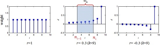
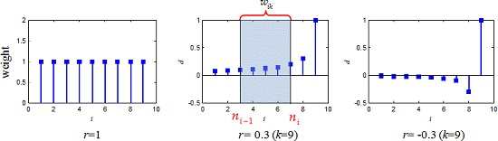
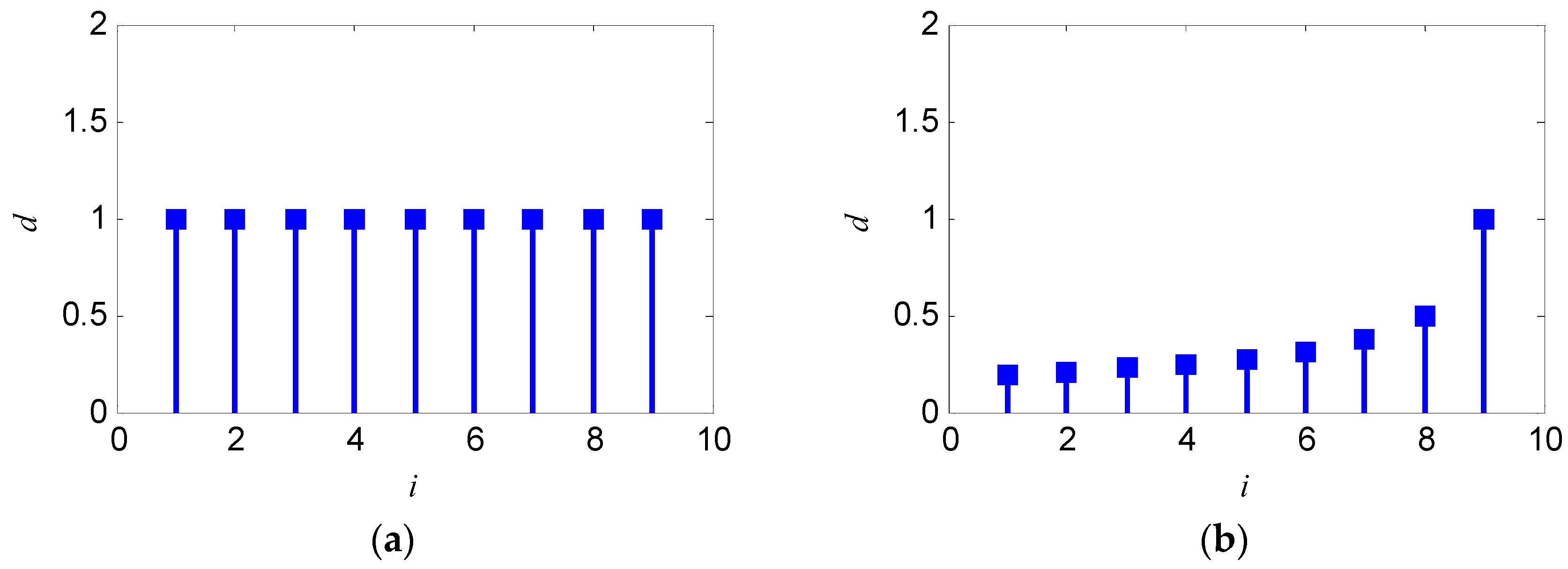
Equation (12) is equal to Equation (4) when r = 1. The original sequence $X^{(0)}$ is accumulated to construct $X^{(r)}$ in the weighted form according to Equation (12). Decreasing r can reduce the weight of previous data and put more emphasis on new data, and the weight of the i-th original data $X^{(0)}(i)$ varied with k in the k-th accumulated data $X^{(r)}(k)$.

2.2. The Traditional NGM(1,1)

Assume that $X^{(0)}=\left\{x^{(0)}(t_1),x^{(0)}(t_2),\mathrm{...},x^{(0)}(t_m)\right\}$ is the original sequence, where $x^{(0)}(t_k)$ denotes the datum at time $t_k$. If all time intervals, $\Delta t_k=t_k-t_{k-1}$ (k = 2, 3, …, m), are not equal to the constant, $X^{(0)}$ is called the non-equidistant sequence.

Based on the first-order non-equidistant accumulated generating operation (1-NAGO) [8], its corresponding accumulated sequence $X^{(1)}$ can be obtained:

$$x^{(1)}(t_k)=x^{(1)}(t_{k-1})+x^{(0)}(t_k)\Delta t_k$$

(13)

The grey differential equation of NGM(1,1) and its whitening equation is defined, respectively:

$$\frac{d{x}^{(1)}}{dt}+a{x}^{(1)}=b$$

(14)

$$x^{(0)}(t_k)+a{z}^{(1)}(t_k)=b$$

(15)

where $z^{(1)}(t_k)$ is the background value, a and b are parameters that can be estimated using the least square method:

$${\left(\begin{array}{cc}a& b\end{array}\right)}^T={\left(B^{T}B\right)}^{-1}{B}^{T}Y$$

(16)

with:

$$B=\left[\begin{array}{ll}-z^{(1)}(t_2)\hfill & 1\hfill \\ -z^{(1)}(t_3)\hfill & 1\hfill \\ \mathrm{...}\hfill & \hfill \\ -z^{(1)}(t_m)\hfill & 1\hfill \end{array}\right],Y=\left[\begin{array}{c}{x}^{(0)}(t_2)\\ x^{(0)}(t_3)\\ \mathrm{...}\\ x^{(0)}(t_m)\end{array}\right]$$

Then the solution of Equation (15) at time $t_k$ is:

$${\widehat{x}}^{(1)}(t_k)=\left[x^{(0)}(t_1)-b/a\right]e^{-a(t_k-t_1)}+b/a$$

(17)

The estimated sequence ${\widehat{X}}^{(0)}$ of the original sequence $X^{(0)}$ can be obtained using the first-order inverse accumulated generating operation [8]:

$${\widehat{x}}^{(0)}(t_k)=\frac{{\widehat{x}}^{(1)}(t_k)-{\widehat{x}}^{(1)}(t_{k-1})}{\Delta t_k}=\frac{1-e^{a\Delta t_k}}{\Delta t_k}\left[x^{(0)}(t_1)-b/a\right]e^{-a(t_k-t_1)}$$

(18)

where ${\widehat{x}}^{(0)}(t_1)=x^{(0)}(t_1)$.

3. The Proposed r-NGM(1,1)

3.1. r-NAGO

The difference between 1-AGO and r-AGO could be found according to Equations (4) and (12). Each value in $X^{(1)}$ is equal to the sum of original data with the same weight of 1, while one in $X^{(r)}$ is equal to the sum of original data with various weights of the accumulated matrix $D^r$, as shown in Figure 1. The weight of the i-th original data $x^{(0)}(i)$ shows a certain tendency with the k-th accumulated data $x^{(r)}(k)$. The closer i reaches k, the more the weight of $x^{(0)}(i)$. Increasing i can reduce the weight of previous values and pay more attention to last values. The weight of the original sequence is a key contributing factor in the accumulated process of the non-equidistant sequence.

Compared Equation (13) with Equation (1), the first-order accumulated data of the non-equidistant sequence are the sum of the original data multiplied by their time distances, while one of the equidistant sequence is the simple sum of the original data. Time distance $\Delta t_k$ is another important factor in 1-NAGO, which is used as the linear weight of each original datum. Therefore, the time distance $\Delta t_k$ and accumulated matrix $D^r$ should be considered introducing into the r-NAGO. Moreover, the time in the non-equidistant sequence needs to be re-sampled due to the discrete form of the accumulated matrix $D^r$, as shown in Equation (11).

For a non-equidistant non-negative sequence $X^{(0)}$, its time sequence is $\left\{t_1,t_2,\mathrm{...},t_m\right\}$. Given the sampled interval T, $t_k$ can be expressed as follows:

$$t_k=t_1+(n_k-1)T$$

(19)

where $n_k$ is the positive integer. Thus, the corresponding time sequence is expressed as $\left\{n_1,n_2,\mathrm{...},n_m\right\}$ and the time distance is rewritten as:

$$\{\begin{array}{l}\Delta n_k=n_k-n_{k-1}(k=2,3,\mathrm{...},m)\hfill \\ \Delta n_1=1\hfill \end{array}$$

(20)

and the original sequence is expressed as $X^{(0)}=\left\{x^{(0)}(n_1),x^{(0)}(n_2),\mathrm{...},x^{(0)}(n_m)\right\}$.

According to the above analysis, the accumulated data $x^{(r)}(n_k)$ at the time $n_k$ should be the weighted sum of the original data from $x^{(0)}(n_1)$ to $x^{(0)}(n_k)$, and the weight of $x^{(0)}(n_i)$ is equal to the sum of the values related to the time distance $\Delta n_i$ in accumulated matrix $D^r$. Therefore, r-NAGO is expressed as follows:

$$x^{(r)}(n_k)={\displaystyle \sum _{i=1}^k{w}_{ik}}{x}^{(0)}(n_i)$$

(21)

where $w_{ik}$ denotes the weight of $x^{(0)}(n_i)$ when calculating $x^{(r)}(n_k)$. It could be defined as follows:

$$w_{ik}={\displaystyle \sum _{j=0}^{\Delta n_i-1}\frac{\Gamma (r+n_k-n_i+j)}{\Gamma (r)\Gamma \left(n_k-n_i+j+1\right)}}$$

(22)

3.2. Negative Fractional Order

After the estimated accumulated sequence ${\widehat{X}}^{(r)}$ is obtained according to grey model, ${\widehat{X}}^{(0)}$ is calculated by the inverse accumulative generating operation:

$${\widehat{X}}^{(0)}=({\widehat{X}}^{(r)}){}^{(-r)}={\widehat{X}}^{(r)}D{}^{(-r)}$$

(23)

According to Equation (10), ${(d^{-r})}_{ik}$ can be obtained:

$$\begin{array}{ll}{(d^{-r})}_{ik}& =\frac{-r(-r+1)\mathrm{...}(-r-1+k-i)}{\left(k-i\right)!}\\ & =\frac{{(-1)}^{k-i}r(r-1)\mathrm{...}(r+1-k+i)}{\left(k-i\right)!}\\ & =\frac{{(-1)}^{k-i}\Gamma \left(r+1\right)}{\Gamma \left(k-i+1\right)\Gamma \left(r-k+i+1\right)}\end{array}$$

(24)

where r > 0. $1/\Gamma \left(k-i+1\right)=0$ if $k<i$, or $1/\Gamma \left(r-k+i+1\right)=0$ if $k-i>r+1$, then ${(d^{-r})}_{ik}$ is equal to 0. The main application of the inverse accumulated generating operation is to revert to the original sequence from the estimated accumulated one.

In traditional grey models, the inherent functional relations of original sequences are deduced through the accumulated generating operation, where the accumulated order is usually positive. However, some actual systems are the increasing processes and the observed data follow potentially approximate exponential rules. Their original sequences are probably exponential incremental sequences, and change rates of some original sequences could even exceed one of exponential functions. Thus, the effectiveness of their accumulated sequences based on the positive accumulated order need to be checked.

Compared Equation (11) with Equation (24), all values in the accumulated matrix $D^r$ are positive when r > 0, while some values are negative when r < 0, shown in Figure 2. The accumulated sequence $X^{(r)}$ with r > 0 increase further their change rates and undermine the grey exponential character in above cases. If the fractional order is negative, their change rates could decrease and follow one of the exponential functions. Thus, a negative fractional order accumulated operation is introduced in this paper. The optimal accumulated sequences are obtained to follow the exponential function better, which could improve the modeling and predicting performance of grey model. The whole accumulated order includes negative and positive numbers.

According to Equations (11) and (24), the element ${(d^r)}_{ik}$ in the whole r-AGO is defined as follows:

$${(d^r)}_{ik}=\{\begin{array}{ll}\frac{\Gamma \left(r+k-i\right)}{\Gamma \left(r\right)\Gamma \left(k-i+1\right)}& (k\ge i，r>0)\\ 0& (k<i)\\ \frac{{(-1)}^{k-i}\Gamma \left(1-r\right)}{\Gamma \left(k-i+1\right)\Gamma \left(i+1-k-r\right)}& (k\ge i，r\le 0)\end{array}$$

(25)

For r = 0, ${(d^r)}_{ik}=1$ if $k=i$, otherwise ${(d^r)}_{ik}=0$ according to Equation (25). Thus, the weight $w_{ik}$ in the whole r-NAGO for the non-equidistant sequence is equal to:

$$w_{ik}=\{\begin{array}{ll}{\displaystyle \sum _{j=0}^{\Delta n_i-1}}\frac{\Gamma (r+n_k-n_i+j)}{\Gamma (r)\Gamma \left(n_k-n_i+j+1\right)}& (r>0)\\ {\displaystyle \sum _{j=0}^{\Delta n_i-1}}\frac{{(-1)}^{n_k-n_i}\Gamma (1-r)}{\Gamma (1-r-n_k+n_i-j)\Gamma \left(n_k-n_i+j+1\right)}& (r\le 0)\end{array}$$

(26)

3.3. r-NGM(1,1)

According to the grey exponential law in grey system theory, the non-equidistant grey model of the r-order accumulated sequence $X^{(r)}$ could be established as the first-order differential equation. It is defined as:

$$\frac{d{x}^{(r)}}{dt}+a{x}^{(r)}=b$$

(27)

Its whitening equation is:

$$\frac{x^{(r)}(n_k)-x^{(r)}(n_{k-1})}{n_k-n_{k-1}}+a{z}^{(r)}(n_k)=b$$

(28)

where the background value $z^{(r)}(n_k)$ is:

$$z^{(r)}(n_k)=\left[x^{(r)}(n_k)+x^{(r)}(n_{k-1})\right]/2$$

(29)

Equation (28) is equal to the traditional NGM(1,1) when r = 1. The accumulated sequence $X^{(r)}$ is substituted into Equation (28) as follows:

$$\{\begin{array}{l}\frac{x^{(r)}(n_2)-x^{(r)}(n_1)}{n_2-n_1}+a{z}^{(r)}(n_2)=b\hfill \\ \frac{x^{(r)}(n_3)-x^{(r)}(n_2)}{n_3-n_2}+a{z}^{(r)}(n_3)=b\hfill \\ \mathrm{...}\hfill \\ \frac{x^{(r)}(n_m)-x^{(r)}(n_{m-1})}{n_m-n_{m-1}}+a{z}^{(r)}(n_m)=b\hfill \end{array}$$

(30)

The coefficients a and b could be estimated based on Equation (16), but the matrix B and Y have to be defined as:

$$B=\left[\begin{array}{ll}-z^{(r)}(n_2)\hfill & 1\hfill \\ -z^{(r)}(n_3)\hfill & 1\hfill \\ \mathrm{...}\hfill & \hfill \\ -z^{(r)}(n_m)\hfill & 1\hfill \end{array}\right],Y=\left[\begin{array}{c}(z^{(r)}(n_2)-z^{(r)}(n_1))/\Delta n_2\\ (z^{(r)}(n_3)-z^{(r)}(n_2))/\Delta n_3\\ \mathrm{...}\\ (z^{(r)}(n_m)-z^{(r)}(n_{m-1}))/\Delta n_m\end{array}\right]$$

Then the solution of Equation (28) should be:

$${\widehat{x}}^{(r)}(n_k)=\left[x^{(0)}(n_1)-\frac{b}{a}\right]e^{-a(n_k-n_1)}+\frac{b}{a}$$

(31)

In order to reduce the effect of the initial condition, Equation (31) could be rewritten as:

$$x^{(r)}(k)=c{e}^{-a(n_k-n_1)}+d$$

(32)

The lease square estimation of parameters c and d satisfies:

$${\left(\begin{array}{cc}c& d\end{array}\right)}^T={(G^{T}G)}^{-1}{G}^{T}H$$

(33)

with:

$$G=\left[\begin{array}{ll}{e}^{-a(n_2-n_1)}\hfill & 1\hfill \\ e^{-a(n_3-n_1)}\hfill & 1\hfill \\ \mathrm{...}\hfill & \hfill \\ e^{-a(n_m-n_1)}\hfill & 1\hfill \end{array}\right],H=\left[\begin{array}{c}{x}^{(r)}(n_2)\\ x^{(r)}(n_3)\\ \mathrm{...}\\ x^{(r)}(n_m)\end{array}\right]$$

After the estimated accumulated sequence ${\widehat{X}}^{(r)}$ is calculated through Equation (32), the estimated values of original sequence ${\widehat{X}}^{(0)}$ could be obtained using r-order inverse accumulated generating operation as follows:

$${\widehat{x}}^{(0)}(n_k,r)=\left[{\widehat{x}}^{(r)}(n_k)-{\displaystyle \sum _{i=1}^{k-1}{w}_{ik}}{\widehat{x}}^{(0)}(n_i)\right]/w_{kk}$$

(34)

where ${\widehat{x}}^{(0)}(n_1,r)=x^{(0)}(n_1)$. ${\widehat{x}}^{(0)}(n_k,r)$ is expressed as the estimated value of the original sequence, where the fractional order is equal to r.

3.4. Optimization of the Accumulated Order

The coefficients $a,b,c$, and $d$ of r-NGM(1,1) in Equation (34) are estimated according to the least square method, but the accumulated order r is expressed as the non-linear function in r-NGM(1,1) and determined comprehensively according to the modeling and predicting accuracy [27]. It could be optimized by means of various methods, such as nonlinear programming and intelligent optimization algorithm. In this paper, the Levenberg–Marquardt algorithm [28] is used to optimize the accumulated order r in r-NGM(1,1).

The Levenberg–Marquardt algorithm is an iterative non-linear least square optimization, whose objective function is to minimize the residual vector constructed with the real values and respective estimated values:

$$\min {\displaystyle \sum _{i=1}^m{\left({\widehat{x}}^{（0）}(n_i,r^{[K]})-x^{(0)}(n_i)\right)}^2}+\mu {(r^{[K]}-r^{[K-1]})}^2$$

(35)

where K is the iterative number, μ is the dumping parameter to affect both the direction and size of the step. μ is divided by a fixed factor if a step is accepted, and it is appropriately multiplied by a factor if a step is rejected.

The accumulated order r is updated at each iteration according to the hereafter expression:

$$r^{[K+1]}=r^{[K]}-{\left(J^{T}J+\mu \right)}^{-1}{J}^{T}E$$

(36)

where J is the Jacobian matrix and E is the residual vector. They can be obtained as:

$$J\left({\widehat{x}}^{(0)},r^{[K]}\right)=\left[\begin{array}{l}\frac{{\widehat{x}}^{(0)}(n_1,r^{[K]})-{\widehat{x}}^{(0)}(n_1,r^{[K-1]})}{r^{[K]}-r^{[K-1]}}\hfill \\ \frac{{\widehat{x}}^{(0)}(n_2,r^{[K]})-{\widehat{x}}^{(0)}(n_2,r^{[K-1]})}{r^{[K]}-r^{[K-1]}}\hfill \\ \mathrm{...}\hfill \\ \frac{{\widehat{x}}^{(0)}(n_m,r^{[K]})-{\widehat{x}}^{(0)}(n_m,r^{[K-1]})}{r^{[K]}-r^{[K-1]}}\hfill \end{array}\right]$$

(37)

$$E=\left[\begin{array}{l}{\widehat{x}}^{(0)}(n_1,r^{[K]})-x^{(0)}(n_1)\hfill \\ {\widehat{x}}^{(0)}(n_2,r^{[K]})-x^{(0)}(n_2)\hfill \\ \mathrm{...}\hfill \\ {\widehat{x}}^{(0)}(n_m,r^{[K]})-x^{(0)}(n_m)\hfill \end{array}\right]$$

(38)

There are two terminal criteria in the optimal procedure, including the maximum iteration and the convergence threshold. The procedure stops when the number of iterations reaches the maximum iteration or the gradient of the objective function falls below the convergence threshold.

Thus, the whole procedure of the optimal r-NGM(1,1) is described in Figure 3.

3.5. Statistical Indicators

The estimated and original sequence is compared in order to demonstrate the modeling and predicting accuracy of the proposed method. Two statistical indicators, including the absolute percent deviation (APD) and root mean square error (RMSE), are used to analyze the accuracy of the proposed model. Their definitions are given below:

$$APD=\frac{1}{s}{\displaystyle \sum _{k=1}^s\left|\frac{x^{(0)}(n_k)-{\widehat{x}}^{(0)}(n_k)}{x^{(0)}(n_k)}\right|}\times 100\%$$

(39)

$$RMSE=\sqrt{\frac{1}{s}{\displaystyle \sum _{k=1}^s{\left(x^{(0)}(n_k)-{\widehat{x}}^{(0)}(n_k)\right)}^2}}$$

(40)

where s is the number of the modeling or predicting data.

4. Computational Cases

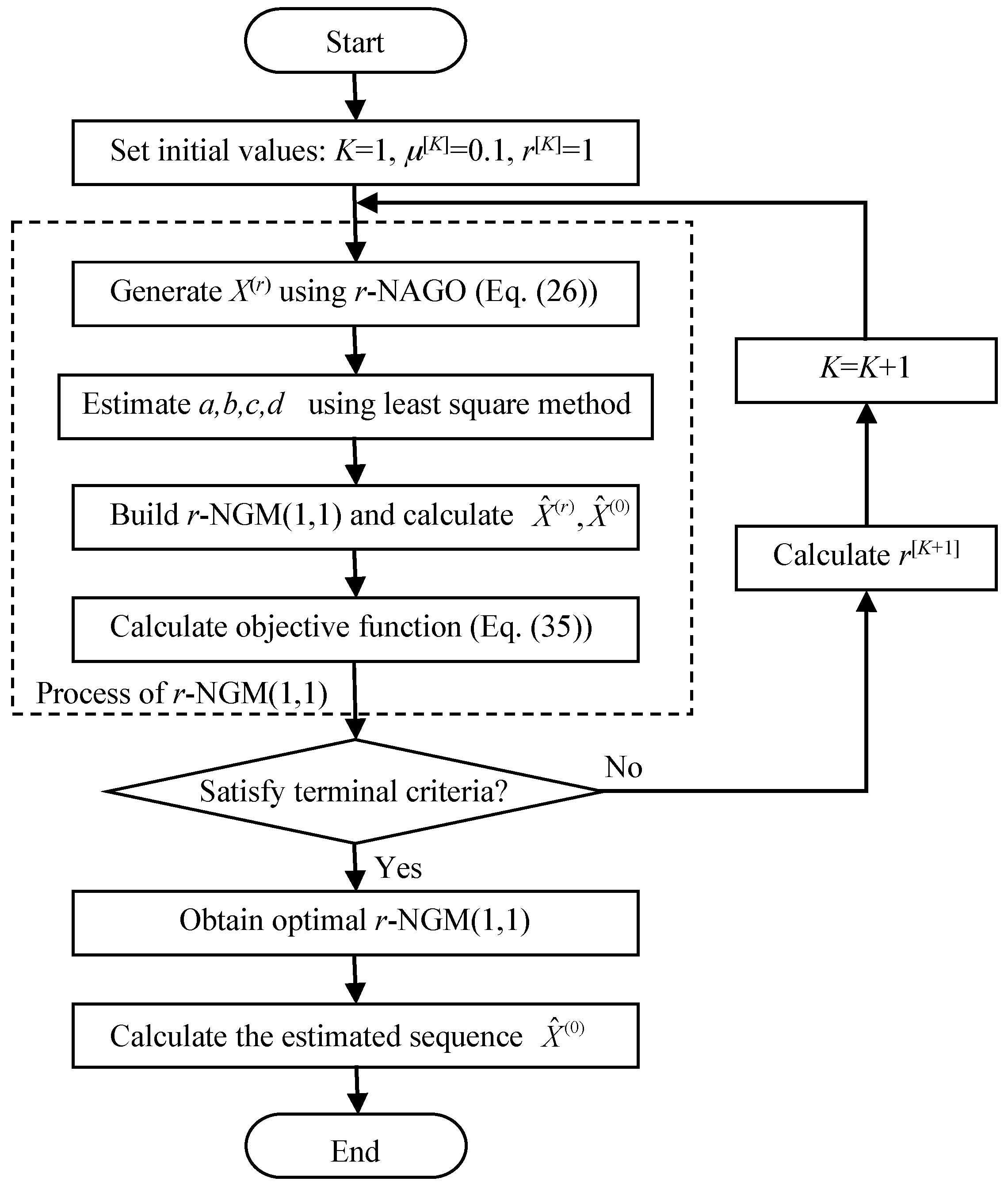
Three practical cases are employed to test the accuracy of the proposed r-NGM(1,1) compared with the traditional NGM(1,1). These non-equidistant sequences are monotonic decreasing, monotonic inceasing, and oscillating, respectively. The maximum iteration is set as 200, the threshold of the gradient is 10⁻⁶, and the factor of is 0.1 in the optimization of the fractional order.

4.1. Case 1

Data comes from [8], which are the experimental data on the fatigue strength (σ₋₁, MPa) of titanium alloy with different temperatures (T_e, °C) under the action of a symmetrical cyclic load, shown in

Table 1. Results of different grey models in Case 1.

k	tk	nk	X(0)	${\widehat{\mathit{X}}}^{\mathbf{(}\mathbf{0}\mathbf{)}}$
				NGM(1,1)	−0.017-NGM(1,1)	0.995-NGM(1,1)	Ref. [8]	Ref. [9]	Ref. [29]
1	100	1	560.00	560.00	560.00	560.00	560.00	560.00	562.87
2	130	4	557.54	557.21	556.79	555.37	554.82	557.73	551.39
3	170	8	536.10	538.35	537.87	538.57	536.49	538.73	535.23
4	210	12	516.10	517.55	517.25	518.14	516.28	517.82	518.06
5	240	15	505.60	500.01	501.95	500.52	499.20	500.21	504.47
6	270	18	486.10	485.45	486.99	485.74	485.02	485.58	490.25
7	310	22	467.40	469.02	467.74	468.97	469.01	469.04	470.24
8	340	25	453.80	453.11	454.01	452.70	453.49	453.08	454.41
9	380	29	436.40	437.78	436.47	436.95	438.52	437.65	432.14

. It is the monotonic decreasing non-equidistant sequence. All data are used to construct different grey models. The sampling interval is set as T = 10 in r-NGM(1,1). Actual and estimated values of several grey models are presented in Table 1 and

Table 2. Statistical results in Case 1.

Grey Model	Modeling Data
	RMSE	APD (%)
NGM(1,1)	2.34	0.35
−0.017-NGM(1,1)	1.55	0.22
0.995-NGM(1,1)	2.37	0.38
Ref. [8]	2.67	0.37
Ref. [9]	2.34	0.35
Ref. [29]	3.31	0.55

.

When the fractional order is limited to be positive, 0.995 is the best accumulated order, which means that 0.995-NGM(1,1) yields the lowest RMSE and APD for this case. When the fractional order is not limited, −0.017-NGM(1,1) provides better performance with APD of 0.22% and RMSE of 1.55, which indicates the reasonable modeling accuracy.

Some modified methods of the traditional NGM(1,1) were proposed to model the fatigue strength data [8,9,29]. The exponential trait and integral [8] was employed to determine the background value so that APD and RMSE were 0.37% and 2.67. Zou [9] put forward the NGM(1,1) based on the reciprocal accumulated generating operation, whose APD and RMSE were 2.34 and 0.35%, respectively. The step-by-step optimum new information method [29] was used to establish NGM(1,1). In this circumstance, its RMSE and APD were 3.31 and 0.55%.

It can be seen that APD obtained using −0.007-NGM(1,1) is less than the traditional NGM(1,1) and three modified NGM(1,1) models [8,9,29]. The proposed r-NGM(1,1) could give an appropriate modeling accuracy for the increasing non-equidistant sequence.

4.2. Case 2

The original sequence is from [30], which is a monotonic increasing non-equidistant sequence. Four data are used to construct different grey models and the fifth datum is predicted. The sampling interval is set as T = 1 in r-NGM(1,1), i.e.,

The background value of the traditional NGM(1,1) is the mean of two adjacent accumulated data, i.e., $z^{(1)}(k)=\left(x^{(1)}(k)+x^{(1)}(k-1)\right)/2$, while the background value of NGM(1,1) in [30] is set as the accumulated values, i.e., $z^{(1)}(k)=x^{(1)}(k)$. Results of different non-equidistant grey models are listed in

Table 3. Results of different grey models in Case 2.

k	tk	nk	X(0)	${\widehat{\mathit{X}}}^{\mathbf{(}\mathbf{0}\mathbf{)}}$
				−0.13-NGM(1,1)	0.93-NGM(1,1)	NGM(1,1)	Ref. [30]
1	50	1	0.7660	0.7660	0.7660	0.7660	0.7660
2	55	6	0.8192	0.8192	0.8198	0.8311	0.8361
3	65	16	0.9063	0.9062	0.9055	0.8871	0.8949
4	80	31	0.9848	0.9848	0.9852	0.9890	0.9908
5	86	37	0.9976	1.0050	1.0360	1.0826	1.0320

and

Table 4. Statistical results in Case 2.

Grey Model	Modeling Data		Predicting Data
	RMSE	APD (%)	RMSE	APD (%)
−0.13-NGM(1,1)	0.0001	0.002	0.007	0.75
0.93-NGM(1,1)	0.001	0.068	0.068	3.85
NGM(1,1)	0.013	1.33	0.085	8.52
Ref. [30]	0.011	1.31	0.034	3.45

.

As can be seen from Table 4, the optimal accumulated order is 0.93 in r-NGM(1,1) when r > 0. The modeling RMSE and APD of 0.93-NGM(1,1) are 0.001 and 0.068% less than that of the traditional NGM(1,1). When r is not limited, the modeling and predicting errors of the −0.13-NGM(1,1) are lowest among these grey models. It gives better performance compared with other grey models. The proposed r-NGM(1,1) could provide the satisfactory modeling and predicting accuracy for the increasing non-equidistant sequences.

4.3. Case 3

The original sequence is collected from [31], which is the strapdown inertial measurement unit. It is an oscillating non-equidistant sequence. Nine data are used to construct different grey models and the tenth datum is predicted. The sampling interval is set as T = 1 in r-NGM(1,1). The modeling and predicting values of different grey models are presented in

Table 5. Results of different grey models in Case 3.

k	tk	nk	X(0)	${\widehat{\mathit{X}}}^{\mathbf{(}\mathbf{0}\mathbf{)}}$
				NGM(1,1)	1.01-NGM(1,1)	−0.01-NGM(1,1)
1	February 2007	1	2.214517	2.214517	2.214517	2.214517
2	May 2007	4	2.209514	2.191818	2.206821	2.205258
3	August 2007	7	2.180164	2.190058	2.188831	2.190021
4	February 2008	13	2.180396	2.187422	2.180613	2.176111
5	August 2008	19	2.180480	2.183911	2.176442	2.174253
6	November 2008	22	2.180469	2.181282	2.175648	2.175123
7	February 2009	25	2.180391	2.179531	2.175813	2.176498
8	October 2009	33	2.170843	2.176325	2.177042	2.180976
9	April 2010	39	2.180387	2.172250	2.179622	2.184262
10	July 2010	42	2.190126	2.169635	2.181756	2.185791

and

Table 6. Statistical results in Case 3.

Model	Modeling Data		Predicting Data
	RMSE	APD (%)	RMSE	APD (%)
NGM(1,1)	0.008	0.30	0.020	0.94
1.01-NGM(1,1)	0.005	0.18	0.008	0.38
−0.01-NGM(1,1)	0.006	0.27	0.004	0.20

.

The optimal accumulated order is 1.01 in r-NGM(1,1) when r is limited to the positive numbers, whose predicting APD and RMSE are 0.38% and 0.008, respectively. −0.01-NGM(1,1) is the best modeling and predicting performance without restriction of the fractional order. Its predicting APD and RMSE are 0.20% and 0.004.

Moreover, the non-equidistant sequence is adjusted to equidistant one by means of cubic spline interpolation and built the grey model GM(1,1) in [31]. The predicting value of the tenth datum was 2.179121, whose relative error was 0.5% higher than that of −0.01-NGM(1,1) and 1.01-NGM(1,1). The proposed r-NGM(1,1) can greatly improve the modeling and predicting accuracy of non-equidistant sequences.

5. Discussion

5.1. Applicability of the Proposed Method

The proposed r-NGM(1,1) in this paper is based on the non-equidistant accumulated generating operation and the basic grey model, GM(1,1), thus, its suitable range and condition is the same as GM(1,1). Firstly the number of the original sequence is more than four in r-NGM(1,1). The second condition is that the r-NGM(1,1) can only be used in positive sequences according to the condition of GM(1,1), but there exist some negative values in the actual applications, especially the accumulated values could be negative when the fractional order is negative. Thus, it is necessary to find a positive value, which is added to the sequence and used to convert into a non-negative sequence. Finally, the original and accumulated sequence should satisfy the quasi-smooth and quasi-exponential checking conditions in conducting the r-NGM(1,1). In case these sequences do not satisfy these conditions, another positive value is added to the sequence and the formed sequence can pass the checking conditions. How to select these two positive values needs to depend on the case analysis.

5.2. The Sampled Interval

The coefficients $a,b,c$, and $d$ of r-NGM(1,1) in Equation (34) are estimated according to the least square method, and the fractional order r is optimized through the Levenberg–Marquardt algorithm in this paper. However, the sampled interval T is given to meet the requirements that every value in a new time sequence is a positive integer according to Equation (19). Different sampled intervals are set to analyze their influences on the modeling and predicting performances of the r-NGM(1,1). Results of three cases are listed in

Table 7. Results of different sampled intervals in three cases.

-	T	nm	Running Time (s)	r	Modeling Data		Predicting Data
					RMSE	APD (%)	RMSE	APD (%)
Case 1	10	29	1.3	−0.017	1.55	0.22	-	-
	1	281	5.9	−0.007	1.52	0.20	-	-
	0.1	2801	275.6	−0.004	1.48	0.21	-	-
Case 2	1	37	2.9	−0.13	0.0001	0.01	0.008	0.75
	0.1	361	5.4	−0.13	0.0005	0.05	0.008	0.84
	0.01	3601	148.7	−0.13	0.0006	0.05	0.008	0.85
Case 3	1	42	1.5	−0.01	0.007	0.27	0.004	0.20
	0.1	411	4.6	−0.01	0.007	0.28	0.001	0.04
	0.01	4101	338.8	−0.01	0.008	0.28	0.001	0.03

under different sampled intervals. Each set of parameters is run five times. The modeling and predicting performances are the most accurate result and the running time is the average one of the five-time runs.

APD and RMSE of the modeling and predicting data are very similar in three cases when the sampled intervals decrease from 10 to 0.01. The optimal fractional orders r are the same in Case 2 and Case 3, while they are different in Case 1, which shows that the sequence in Case 1 is more sensitive to the fractional order. Moreover, the maximal time $n_m$ and running time increase dramatically when the sampled interval decreases. The sampled intervals affect the modeling and predicting performance of r-NGM(1,1) less, so the main factor to select the sampled interval is the running time.

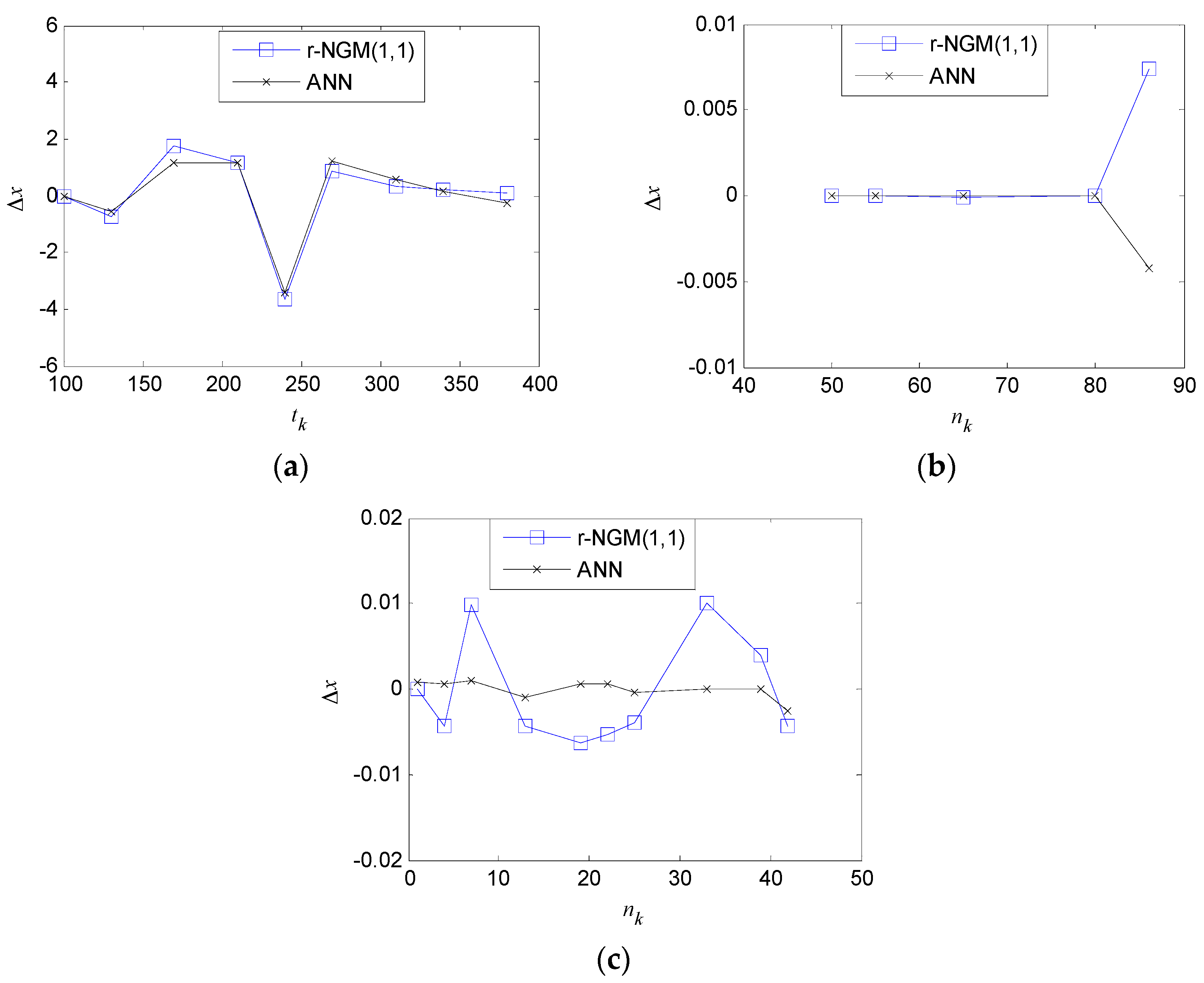
5.3. Comparison with Other Method

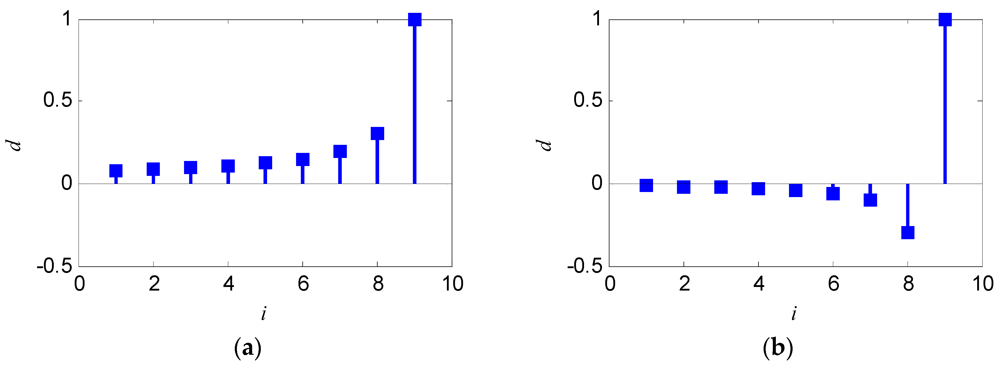
An artificial neural network (ANN) [32] is employed to compare with the proposed r-NGM(1,1) in this paper. Figure 4 shows errors Δx between the original and estimated values obtained by two models, and their comparison results are listed in

Table 8. Comparison results of different models.

-			Case 1	Case 2	Case 3
r-NGM(1,1)	r		−0.017	−0.13	−0.01
	Modeling data	RMSE	1.5531	0.0001	0.0064
		APD (%)	0.2159	0.0037	0.2744
	Predicting data	RMSE	-	0.0074	0.0043
		APD (%)	-	0.7418	0.1979
ANN	Number of hidden nodes		2	2	4
	Modeling data	RMSE	1.3495	0	0.0006
		APD (%)	0.1868	0	0.0252
	Predicting data	RMSE	-	0.0042	0.0025
		APD (%)	-	0.4210	0.1146

. A three-layered ANN is used to predict the non-equidistant sequences, consisting of an input layer, hidden layer, and output layer. The number of neurons in the hidden layer is chosen empirically by adjusting the number of neurons until the effective number of parameters reaches a constant value.

As shown in Figure 4 and Table 8, the RMSE and APD of the ANN is smaller than one of the proposed r-NGM(1,1), which indicates less deviation between the estimated and original values for the ANN. A greater number of neurons in the hidden layer in the ANN could provide more accurate prediction, but significantly increase the model complexity. The proposed grey model is simpler than the neural network under the same modeling and predicting performance. Compared with the ANN, the proposed r-NGM(1,1) gives better performance with satisfactory accuracy and concise explicit models for non-equidistant sequences.

6. Conclusions and Future Work

A novel fractional-order non-equidistant grey model, r-NGM(1,1), is proposed to deal with the predicting problem of non-equidistant sequences. The fractional-order non-equidistant accumulated generating operation is developed to extend the application of grey models with fractional order accumulation. Some cases have been carried out to evaluate the proposed r-NGM(1,1) in comparison with the traditional NGM(1,1). Results show that the proposed r-NGM(1,1) remarkably increases the modeling and predicting accuracy of non-equidistant sequence.

The proposed r-NGM(1,1) is constructed through the partially-known information, so it is not more suitable for the systems with the distinct inherent mechanism, and it is difficult to obtain more accuracy for the long-term prediction due to the limitation of time effect. Moreover, the effectiveness of the proposed r-NGM(1,1) is only validated based on some practical cases in this paper. More cases and applications are employed to validate the modeling and predicting performance of r-NGM(1,1). It is important to give the theoretical analysis of r-NAGO and r-NGM(1,1), which will be carried out in the next work. The proposed r-NGM(1,1) in this paper is still based on first-order grey differential equations with r-AGO, so it is necessary to further discuss its relationship with the fractional-order grey differential equations with 1-AGO or fractional-order ones with r-AGO.

As a future work, optimal initial values and background values should be considered to further improve the modeling and predicting performance of r-NGM(1,1), and an effective optimization technique is developed to derive the global optimal solutions of the fractional order and coefficients in r-NGM(1,1) due to the nonlinear objective function shown in Equation (35). Meanwhile, the proposed r-NAGO is introduced into other non-equidistant grey models, such as the discrete grey model, grey Verhulst model, and grey power model.

References

1. Frida, E. Non-Uniform Sampling in Statistical Signal Processing. Ph.D. Thesis, Linköpings Universitet, Linköping, Sweden, 2007. [Google Scholar]
2. Candès, E.; Wakin, M. An introduction to compressive sampling. IEEE Signal Process. 2008, 25, 21–30. [Google Scholar] [CrossRef]
3. Yang, Y.; Nagarajaiah, S. Output-only modal identification by compressed sensing: Non-uniform low-rate random sampling. Mech. Syst. Signal Process. 2015, 56–57, 15–34. [Google Scholar] [CrossRef]
4. Deng, J. Introduction grey system theory. J. Grey Syst. 1989, 1, 1–24. [Google Scholar]
5. Liu, S.; Forrest, J.; Yang, Y. A brief introduction to grey systems theory. Grey Syst. Theory Appl. 2012, 2, 89–104. [Google Scholar] [CrossRef]
6. Xiao, X.; Peng, K. Research on generalized non-equidistance GM(1,1) model based on matrix analysis. Grey Syst. Theory Appl. 2011, 1, 87–96. [Google Scholar] [CrossRef]
7. Chang, C.-J.; Li, D.-C.; Chen, C.-C.; Chen, C.-S. A forecasting model for small non-equigap data sets considering data weights and occurrence possibilities. Comput. Ind. Eng. 2014, 67, 139–145. [Google Scholar] [CrossRef]
8. Dai, W.Z.; Li, J.F. Modeling research on non-equidistance GM(1,1) model. Syst. Eng. Theory Pract. 2005, 25, 89–93. (In Chinese) [Google Scholar]
9. Zou, R.B.; Mou, Z.X.; Wei, Y. The non-equidistant grey GRM(1, 1) model and its application. Int. J. Mod. Nonlinear Theory Appl. 2012, 1, 51–54. [Google Scholar] [CrossRef]
10. Kang, X.; Wei, Y.; Shen, Y. The class ratio modeling method of non-equigap GM(1,1) model. In Proceedings of the 2009 International Symposium on Information Processing, Huangshan, China, 21–23 August 2009; pp. 286–289.
11. Zeng, X.Y.; Shu, L. Non-equidistant GM(1,1) based on accumulated method and its properties. J. Grey Syst. 2012, 15, 139–144. [Google Scholar]
12. Wang, Q.F. Parameter estimation of non-equidistant GM(1,1) model based on the Euler formula. In Proceedings of the 2009 IEEE International Conference on Grey Systems and Intelligent Services, Nanjing, China, 10–12 November 2009; pp. 378–382.
13. Li, G.D.; Yamaguchi, D.; Nagai, M. Non-equidistance grey model based on grey interval weighting accumulated generating operation. In Proceedings of the 2006 International Conference on Machine Learning, Models, Technologies & Applications, Las Vegas, NV, USA, 26–29 June 2006; pp. 180–188.
14. Shu, H.; Dang, Y.; Xiong, P. Research on characteristics of grey non-equidistant Verhulst model. In Proceedings of the 2011 IEEE International Conference on Grey Systems and Intelligent Services, Nanjing, China, 15–18 September 2011; pp. 209–212.
15. Yong, H.; Wei, Y. The optimization of the non-equigap DGM(2,1) model. J. Grey Syst. 2011, 14, 41–46. [Google Scholar]
16. Wang, Z.X.; Dang, Y.G.; Liu, S.F. Non-equidistant GM(1,1) power model and its application in engineering. Chin. Eng. Sci. 2012, 14, 98–102. (In Chinese) [Google Scholar]
17. Monje, C.A.; Chen, Y.Q.; Vinagre, B.M.; Xue, D.; Feliu-Batlle, V. Fractional-Order Systems and Controls: Fundamentals and Applications; Springer: London, UK, 2010. [Google Scholar]
18. Sierociuk, D.; Dzielinski, A. Fractional kalman filter algorithm for the states, parameters and order of fractional system estimation. Int. J. Appl. Math. Comput. Sci. 2006, 16, 129–140. [Google Scholar]
19. Valério, D.; Trujillo, J.J.; Rivero, M.; Machado, J.A.T.; Beleanu, D. Fractional calculus: a survey of useful formulas. Eur. Phys. J. Spec. Top. 2013, 222, 1827–1846. [Google Scholar] [CrossRef]
20. Wu, L.F.; Liu, S.F.; Yao, L.G.; Yana, S.; Liua, D. Grey system model with the fractional order accumulation. Commun. Nonlinear Sci. Numer. Simul. 2013, 18, 1775–1785. [Google Scholar] [CrossRef]
21. Mao, S.; Gao, M.; Xiao, X. Fractional order accumulation time-lag GM(1,N,τ) model and its application. Syst. Eng. Theory Pract. 2015, 35, 430–436. (In Chinese) [Google Scholar]
22. Liu, J.; Liu, S.; Fang, Z. Fractional-order reverse accumulation generation GM(1,1) model and its applications. J. Grey Syst. 2015, 27, 52–62. [Google Scholar]
23. Yang, B.H.; Zhao, J.S. Fractional order discrete grey GM(1,1) power model and its application. Control Decis. 2015, 30, 1264–1268. (In Chinese) [Google Scholar]
24. Wu, L.F.; Liu, S.F.; Cui, W.; Liu, D.-L.; Yao, T.-X. Non-homogenous discrete grey model with fractional-order accumulation. Neural Comput. Appl. 2014, 25, 1215–1221. [Google Scholar] [CrossRef]
25. Mao, S.H.; Gao, M.Y.; Xiao, X.P.; Zhu, M. A novel fractional grey system model and its application. Appl. Math. Model. 2016, 40, 5063–5076. [Google Scholar] [CrossRef]
26. Meng, W.; Li, Q.; Zeng, B. Study on fractional order grey reducing generation operator. Grey Syst. Theory Appl. 2016, 6, 80–95. [Google Scholar] [CrossRef]
27. Shen, Y.; Qin, P. Optimization of grey model with the fractional order accumulated generation. J. Grey Syst. 2014, 17, 127–132. [Google Scholar]
28. Ueda, K.; Yamashita, N. On a global complexity bound of the Levenberg-Marquardt method. J. Opt. Theory Appl. 2010, 147, 443–453. [Google Scholar] [CrossRef]
29. Luo, Y.X. Non-equidistant step by step optimum new information GM(1,1) and its application. Syst. Eng. Theory Pract. 2010, 30, 2254–2258. (In Chinese) [Google Scholar]
30. He, X.; Sun, G.; Li, L. New rules for an accumulated generating operation and inverse accumulated generating operation of gray series. J. Wuhan Univ. Technol. 2002, 24, 26–28. (In Chinese) [Google Scholar]
31. Zhang, Z.J.; Liu, J.Y.; Ma, X.W. Modeling forecast of the SIMU error coefficient Based on unequal interval gray model. Missiles Space Veh. 2011, 5, 40–42. (In Chinese) [Google Scholar]
32. Svitlana, G. Neural networks performance in exchange rate prediction. Neurocomputing 2016, 172, 446–452. [Google Scholar]
Figure 1. Weights of the original data in AGO: (a) 1-AGO; and (b) r-AGO (r = 0.5, k = 9).
Entropy 18 00227 g001
Figure 2. Weights of the original data in r-AGO: (a) r = 0.3, k = 9; and (b) r = −0.3, k = 9.
Entropy 18 00227 g002
Figure 3. Flow diagram of the optimal r-NGM(1,1).
Entropy 18 00227 g003
Figure 4. Errors of the estimated sequence with two methods: (a) Case 1; (b) Case 2; and (c) Case 3.
Entropy 18 00227 g004