Constant Slope Maps and the Vere-Jones Classification

Abstract

We study continuous countably-piecewise monotone interval maps and formulate conditions under which these are conjugate to maps of constant slope, particularly when this slope is given by the topological entropy of the map. We confine our investigation to the Markov case and phrase our conditions in the terminology of the Vere-Jones classification of infinite matrices.

1. Introduction

For $a,b\in \mathbb{R}$, $a<b$, a continuous map $T:[a,b]\to \mathbb{R}$ is said to be piecewise monotone if there are $k\in \mathbb{N}$ and points $a=c_0<c_1<\cdots <c_{k-1}<c_k=b$, such that T is monotone on each $[c_i,c_{i+1}]$, $i=0,\dots ,k-1$. A piecewise monotone map T has constant slopes if $|T^{\prime }(x)|=s$ for all $x\ne c_i$.

The following results are well known for piecewise monotone interval maps:

Theorem 1 

([1,2]). If $T:[0,1]\to [0,1]$ is piecewise monotone and $h_{top}(T)>0$, then T is semi-conjugate via a continuous non-decrease onto map $\phi :[0,1]\to [0,1]$ to a map S of constant slope $e^{h_{top}(T)}$. The map ϕ is a conjugacy (ϕ is strictly increasing) if T is transitive.

Theorem 2 

([3]). If T has a constant slope s, then $h_{top}(T)=max(0,logs)$.

For continuous interval maps with a countably-infinite number of pieces of monotonicity, neither theorem is true; for examples, see [4] and [5]. One of the few facts that remains true in the countably-piecewise monotone setting is:

Proposition 1 

([6]). If T is s-Lipschitz, then $h_{top}(T)\le max\{0,logs\}$.

A continuous interval map T has constant slope s if $|T^{\prime }(x)|=s$ for all but countably many points.

The question we want to address is when a continuous countably-piecewise monotone interval map T is conjugate to a map of constant slope λ. Particular attention will be given to the case when a slope is given by the topological entropy of T, which we call linearizability:

Definition 1. 

A continuous map $T:[0,1]\to [0,1]$ is said to be linearizable if it is conjugate to an interval map of constant slope $\lambda =e^{h_{top}(T)}$.

We will confine ourselves to the Markov case and explore what can be said if only the transition matrix of a countably-piecewise monotone map is known in terms of the Vere-Jones classification [7], refined by [8].

The structure of our paper is as follows.

In Section 2 ($\mathcal{C}\mathcal{P}\mathcal{M}\mathcal{M}$: the class of countably-piecewise monotone Markov maps), we make precise the conditions on continuous interval maps under which we conduct our investigation; the set of all such maps will be denoted by $\mathcal{C}\mathcal{P}\mathcal{M}\mathcal{M}$ (for countably-piecewise monotone Markov). In particular, we introduce a slack countable Markov partition of a map and distinguish between the operator and non-operator type respectively.

In Section 3 (conjugacy of a map from $\mathcal{C}\mathcal{P}\mathcal{M}\mathcal{M}$ to a map of constant slope), we rephrase the key equivalence from [9] (Theorem 2.5): for the sake of completeness, we formulate Theorem 3, which relates the existence of a conjugacy to an “eigenvalue equation” (5), using both classical and slack countable Markov partitions; see Definition 2.

Section 4 (the Vere-Jones classification) is devoted to the Vere-Jones classification [7] that we use as a crucial tool in most of our proofs in later sections.

In Section 5 (entropy and the Vere-Jones classification in $\mathcal{C}\mathcal{P}\mathcal{M}\mathcal{M}$), we show in Proposition 8 that the topological entropy of a map in question and (the logarithm of) the Perron value of its transition matrix coincide. Using this fact, we are able to verify in Proposition 9 that all of the transition matrices of a map corresponding to all of the possible Markov partitions of that map belong to the same class in the Vere-Jones classification; so we can speak about the Vere-Jones classification of a map from $\mathcal{C}\mathcal{P}\mathcal{M}\mathcal{M}$.

In Section 6 (linearizability), we present the main results of this text. We start with Proposition 10 showing two basic properties of a λ-solution of Equation (5) and Theorem 7 on locally eventually onto (leo) maps; see Definition 4. Afterwards, we describe conditions under which a local window perturbation—Theorems 8 and 9, resp. a global window perturbation—Theorems 10 and 11 results in a linearizable map.

In Section 7 (examples), various examples illustrating linearizability/conjugacy to a map of constant slope in the Vere-Jones classes are presented.

2. $\mathcal{C}\mathcal{P}\mathcal{M}\mathcal{M}$: The Class of Countably Piecewise Monotone Markov Maps

Definition 2. 

A countable Markov partition $\mathcal{P}$ for a continuous map $T:[0,1]\to [0,1]$ consists of closed intervals with the following properties:

• Two elements of $\mathcal{P}$ have pairwise disjoint interiors, and $[0,1]\backslash \bigcup \mathcal{P}$ is at most countable.
• The partition $\mathcal{P}$ is finite or countably-infinite;
• ${T|}_i$ is monotone for each $i\in \mathcal{P}$ (classical Markov partition) or piecewise monotone for each $i\in \mathcal{P}$; in the latter case, we will speak of a slack Markov partition.
• For every $i,j\in \mathcal{P}$ and every maximal interval $i^{\prime }\subset i$ of monotonicity of T, if $T(i^{\prime })\cap j^{\circ }\ne \varnothing$, then $T(i^{\prime })\supset j$.

Remark 1. 

The notion of a slack Markov partition will be useful in later sections of this paper, where we will work with window perturbations. If $\#\mathcal{P}=\infty$, then the ordinal type of $\mathcal{P}$ need not be $\mathbb{N}$ or $\mathbb{Z}$.

Definition 3. 

The class $\mathcal{C}\mathcal{P}\mathcal{M}\mathcal{M}$ is the set of continuous interval maps $T:[0,1]\to [0,1]$ satisfying:

• T is topologically mixing, i.e., for every open sets $U,V$, there is an n, such that $T^m(U)\cap V\ne \varnothing$ for all $m\ge n$.
• T admits a countably-infinite Markov partition.
• $h_{top}(T)<\infty$.

Remark 2. 

Since $T\in \mathcal{C}\mathcal{P}\mathcal{M}\mathcal{M}$ is topologically mixing by definition, it cannot be constant on any subinterval of $[0,1]$.

Definition 4. 

A map $T\in \mathcal{C}\mathcal{P}\mathcal{M}\mathcal{M}$ is called leo (locally eventually onto) if for every nonempty open set U, there is an $n\in \mathbb{N}$, such that $f^n(U)=[0,1]$.

Remark 3. 

Let $T:[0,1]\to [0,1]$ be a piecewise monotone Markov map, i.e., such that orbits of turning points and endpoints $\{0,1\}$ are finite. Those orbits naturally determine a finite Markov partition for T. This partition can be easily be refined, in infinite ways, to countably-infinite Markov partitions. If T is topologically mixing and continuous, then we will consider T as an element of $\mathcal{C}\mathcal{P}\mathcal{M}\mathcal{M}$.

Proposition 2. 

Let $T\in \mathcal{C}\mathcal{P}\mathcal{M}\mathcal{M}$ with a Markov partition $\mathcal{P}$. For every pair $i,j\in \mathcal{P}$ satisfying $T(i)\supset j$, there exist a maximal $\kappa =\kappa (i,j)\in \mathbb{N}$ and intervals $i_1,\dots ,i_{\kappa }\subset i$ with pairwise disjoint interiors, such that ${T|}_{i_{\ell }}$ is monotone and $T(i_{\ell })\supset j$ for each $\ell =1,\dots ,\kappa$.

Proof. 

Since $T\in \mathcal{C}\mathcal{P}\mathcal{M}\mathcal{M}$ is topologically mixing, it is not constant on any subinterval of $[0,1]$. Fix a pair $i,j\in \mathcal{P}$ with $T(i)\supset j$. Since T is continuous, there has to be at least one, but at most a finite number of pairwise disjoint subintervals of i satisfying the conclusion. ☐

For a given $T\in \mathcal{C}\mathcal{P}\mathcal{M}\mathcal{M}$ with a Markov partition $\mathcal{P}$, applying Proposition 2, we associate with $\mathcal{P}$ the transition matrix $M=M(T)={(m_{ij})}_{i,j\in \mathcal{P}}$ defined by:

$$m_{ij}=\left\{\begin{array}{cc}\kappa (i,j)\hfill & \text{if}T(i)\supset j\hfill \\ 0\hfill & \text{otherwise}\hfill \end{array}\right.$$

(1)

If $\mathcal{P}$ is a classical Markov partition of some $T\in \mathcal{C}\mathcal{P}\mathcal{M}\mathcal{M}$, then $m_{ij}\in \{0,1\}$ each $i,j\in \mathcal{P}$.

Remark 4. 

For the sake of clarity, we will write $(T,\mathcal{P},M)\in {\mathcal{C}\mathcal{P}\mathcal{M}\mathcal{M}}^{*}$ when a map $T\in \mathcal{C}\mathcal{P}\mathcal{M}\mathcal{M}$, a concrete Markov partition $\mathcal{P}$ for T and its transition matrix $M=M(T)$ with respect to $\mathcal{P}$ are assumed.

For an infinite matrix M indexed by a countable index set $\mathcal{P}$, we can consider the powers $M^n={(m_{ij}(n))}_{i,j\in \mathcal{P}}$ of M:

$$M^0=E={({\delta }_{ij})}_{i,j\in \mathcal{P}},M^n={\left(\sum _{k\in \mathcal{P}}{m}_{ik}{m}_{kj}(n-1)\right)}_{i,j\in \mathcal{P}},n\in \mathbb{N}$$

(2)

Proposition 3. 

Let $(T,\mathcal{P},M)\in {\mathcal{C}\mathcal{P}\mathcal{M}\mathcal{M}}^{*}$.

(i) 

For each $n\in \mathbb{N}$ and $i,j\in \mathcal{P}$, the entry $m_{ij}(n)$ of $M^n$ is finite.

(ii) 

The entry $m_{ij}(n)=m$ if and only if there are exactly m subintervals $i_1$, …, $i_m$ of i with pairwise disjoint interiors, such that $T^n(i_k)\supset j$, $k=1,\dots ,m$.

Proof. 

(i)

From the continuity of T and the definition of M, it follows that the sum ${\sum }_{i\in \mathcal{P}}{m}_{ij}$ is finite for each $j\in \mathcal{P}$, which directly implies (i).

(ii)

For $n=1$, this is given by the relation (1) defining the matrix M. The induction step follows from (2) of the product of the nonnegative matrices M and $M^{n-1}$.

☐

A matrix M indexed by the elements of $\mathcal{P}$ represents a bounded linear operator $\mathcal{M}$ on the Banach space ${\ell }^1={\ell }^1(\mathcal{P})$ of summable sequences indexed by $\mathcal{P}$, provided that the supremum of the columnar sums is finite. Then, $\mathcal{M}$ is realized through left multiplication:

$$\begin{array}{cc}& \mathcal{M}(v):={\left(\sum _{j\in \mathcal{P}}{m}_{ij}{v}_j\right)}_{i\in \mathcal{P}},v\in {\ell }^1(\mathcal{P})\hfill \\ & \parallel \mathcal{M}\parallel =\underset{j}{sup}\sum _i{m}_{ij}\hfill \end{array}$$

(3)

The matrix $M^n$ represents the n-th power ${\mathcal{M}}^n$ of $\mathcal{M}$ and by Gelfand’s formula, the spectral radius $r_{\mathcal{M}}={lim}_{n\to \infty }{\parallel {\mathcal{M}}^n\parallel }^{\frac{1}{n}}$.

Remark 5. 

If $(T,\mathcal{P},M)\in {\mathcal{C}\mathcal{P}\mathcal{M}\mathcal{M}}^{*}$, the supremum in (3) is finite if and only if:

$$\exists K>0\forall y\in [0,1]:\#T^{-1}(y)\le K$$

(4)

Since this condition does not depend on a concrete choice of $\mathcal{P}$, we will say the map T is of an operator type when the condition (4) is fulfilled and of a non-operator type otherwise.

3. Conjugacy of a Map from $\mathcal{C}\mathcal{P}\mathcal{M}\mathcal{M}$ to a Map of Constant Slope

This section is devoted to the fundamental observation regarding a possible conjugacy of an element of $\mathcal{C}\mathcal{P}\mathcal{M}\mathcal{M}$ to a map of constant slope. It is presented in Theorem 3.

Let $(T,\mathcal{P},M)\in {\mathcal{C}\mathcal{P}\mathcal{M}\mathcal{M}}^{*}$. We are interested in positive real numbers λ and nonzero nonnegative sequences ${(v_i)}_{i\in \mathcal{P}}$ satisfying $Mv=\lambda v$, or equivalently:

$$\forall i\in \mathcal{P}:\sum _{j\in \mathcal{P}}{m}_{ij}{v}_j=\lambda v_i$$

(5)

Definition 5. 

A nonzero nonnegative sequence $v={(v_i)}_{i\in \mathcal{P}}$ satisfying (5) will be called a λ-solution (for M). If in addition $v\in {\ell }^1(\mathcal{P})$, it will be called a summable λ-solution (for M).

Remark 6. 

Since every $T\in \mathcal{C}\mathcal{P}\mathcal{M}\mathcal{M}$ is topologically mixing, any nonzero nonnegative λ-solution is in fact positive: if $v={(v_i)}_{i\in \mathcal{P}}$ solves Equation (5), $k,j\in \mathcal{P}$ and $v_j>0$, then by Proposition 3(ii) for some sufficiently large n, ${\lambda }^n{v}_k\ge m_{kj}(n)v_j>0$.

Let ${\mathcal{C}\mathcal{P}\mathcal{M}\mathcal{M}}_{\lambda }$ denote the class of all maps from $\mathcal{C}\mathcal{P}\mathcal{M}\mathcal{M}$ of constant slope λ, i.e., $S\in {\mathcal{C}\mathcal{P}\mathcal{M}\mathcal{M}}_{\lambda }$ if $|S^{\prime }(x)|=s$ for all, but countably many points.

The core of the following theorem has been proven in [9] (Theorem 2.5). Since we will work with maps from $\mathcal{C}\mathcal{P}\mathcal{M}\mathcal{M}$ that are topologically mixing, we use topological conjugacies only; see [10] (Proposition 4.6.9). The theorem will enable us to change freely between classical/slack Markov partitions of the map in question.

Theorem 3. 

Let $T\in \mathcal{C}\mathcal{P}\mathcal{M}\mathcal{M}$. The following conditions are equivalent.

(i) 

For some $\lambda >1$, the map T is conjugate via a continuous increasing onto map $\psi :[0,1]\to [0,1]$ to some map $S\in {\mathcal{C}\mathcal{P}\mathcal{M}\mathcal{M}}_{\lambda }$.

(ii) 

For some classical Markov partition $\mathcal{P}$ for T, there is a positive summable λ-solution $u={(u_i)}_{i\in \mathcal{P}}$ of Equation (5).

(iii) 

For every classical Markov partition $\mathcal{P}$ for T, there is a positive summable λ-solution $u={(u_i)}_{i\in \mathcal{P}}$ of Equation (5).

(iv) 

For every slack Markov partition $\mathcal{Q}$ for T, there is a positive summable λ-solution $v={(v_i)}_{i\in \mathcal{Q}}$ of Equation (5).

(v) 

For some slack Markov partition $\mathcal{Q}$ for T, there is a positive summable λ-solution $v={(v_i)}_{i\in \mathcal{Q}}$ of Equation (5).

Remark 7. 

Recently, Misiurewicz and Roth [11] have pointed out that if v is a λ-solution of Equation (5) that is not summable, then the map T is conjugate to a map of constant slope defined on the real line or half-line.

Remark 8. 

Let $T\in \mathcal{C}\mathcal{P}\mathcal{M}\mathcal{M}$ be piecewise monotone with a finite Markov partition. It is well known (see, [10] (Theorem 4.4.5) and [12] (Theorem 0.16)) that the corresponding Equation (5) has a positive $e^{h_{top}(T)}$-solution, which is trivially summable. By Theorem 3, it is also true for any countably infinite Markov partition for T.

Proof of Theorem 3. 

The equivalence of (i), (ii) and (iii) has been proven in [9]. Since (iv) implies (iii) and (v), it suffices to show that (iii) implies (iv) and (v) implies (ii).

(iii)$\stackrel{\hspace{1em}}{\Rightarrow }$(iv). Let us assume that $\mathcal{Q}$ is a slack Markov partition for T. Obviously, there is a classical partition $\mathcal{P}$ for T which is finer than $\mathcal{Q}$, i.e., every element of $\mathcal{P}$ is contained in some element of $\mathcal{Q}$. Using (iii), we can consider a positive summable λ-solution $u={(u_i)}_{i\in \mathcal{P}}$ of Equation (5). Let $v={(v_i)}_{i\in \mathcal{Q}}$ be defined as:

$$v_i=\sum _{i^{\prime }\subset i}{u}_{i^{\prime }}$$

Clearly, the positive sequence $v={(v_i)}_{i\in \mathcal{Q}}$ is from ${\ell }^1(\mathcal{Q})$. Denoting ${(m_{ij}^{\mathcal{P}})}_{i,j\in \mathcal{P}}$ and ${(m_{ij}^{\mathcal{Q}})}_{i,j\in \mathcal{Q}}$ the transition matrices corresponding to the partitions $\mathcal{P}$, $\mathcal{Q}$, we can write:

$$\begin{array}{cc}\hfill \lambda v_i& =\lambda \sum _{i^{\prime }\subset i}{u}_{i^{\prime }}=\sum _{i^{\prime }\subset i}\lambda u_{i^{\prime }}=\sum _{i^{\prime }\subset i}\sum _{k\in \mathcal{Q}}\sum _{k^{\prime }\subset k}{m}_{i^{\prime }{k}^{\prime }}^{\mathcal{P}}{u}_{k^{\prime }}\hfill \\ & =\sum _{k\in \mathcal{Q}}\left(\sum _{k^{\prime }\subset k}{u}_{k^{\prime }}\right)\left(\sum _{i^{\prime }\subset i}{m}_{i^{\prime }{k}^{\prime }}^{\mathcal{P}}\right)=\sum _{k\in \mathcal{Q}}{m}_{ik}^{\mathcal{Q}}{v}_k,\hfill \end{array}$$

(6)

where the equality $m_{ik}^{\mathcal{Q}}={\sum }_{i^{\prime }\subset i}{m}_{i^{\prime }{k}^{\prime }}^{\mathcal{P}}$ follows from the Markov property of T on $\mathcal{P}$ and $\mathcal{Q}$:

$$\text{if}T(i^{\prime })\supset k^{\prime }\text{for}\text{some}{k}^{\prime }\subset k\text{then}\text{also}T(i^{\prime })\supset k$$

(7)

Therefore, by Equation (6), for a given slack Markov partition $\mathcal{Q}$ (for T), we find a positive summable λ-solution $v={(v_i)}_{i\in \mathcal{Q}}$ of Equation (5).

(v)$\stackrel{\hspace{1em}}{\Rightarrow }$(ii). Assume that for some slack Markov partition $\mathcal{Q}$ for T, there is a positive summable λ-solution $v={(v_i)}_{i\in \mathcal{Q}}$ of Equation (5). As in the previous part, we can consider a classical Markov partition $\mathcal{P}$ finer than $\mathcal{Q}$. Using again the property (7), let us put:

$$u_{i^{\prime }}=\sum _{T(i^{\prime })\supset j}{v}_j,i^{\prime }\in \mathcal{P}$$

(8)

Then, $u={(u_{i^{\prime }})}_{i^{\prime }\in \mathcal{P}}$ is positive, and we will show that it is a summable λ-solution of Equation (5). Fix an $i^{\prime }\in \mathcal{P}$, and use the property (7) for $j\in \mathcal{Q}$ for which $T(i^{\prime })\supset j$. Then:

$$\lambda v_j=\sum _{k\in \mathcal{Q}}{m}_{jk}^{\mathcal{Q}}{v}_k=\sum _{j^{\prime }\subset j}\sum _{T(j^{\prime })\supset \ell }{v}_{\ell }=\sum _{j^{\prime }\subset j}{m}_{i^{\prime }{j}^{\prime }}^{\mathcal{P}}\sum _{T(j^{\prime })\supset \ell }{v}_{\ell }=\sum _{j^{\prime }\subset j}{m}_{i^{\prime }{j}^{\prime }}^{\mathcal{P}}{u}_{j^{\prime }}$$

(9)

Hence, summing Equation (9) through all j’s from $\mathcal{Q}$ that are T-covered by $i^{\prime }\in \mathcal{P}$, we obtain with the help of Equation (8),

$$\lambda u_{i^{\prime }}=\sum _{T(i^{\prime })\supset j}\lambda v_j=\sum _{T(i^{\prime })\supset j}\sum _{j^{\prime }\subset j}{m}_{i^{\prime }{j}^{\prime }}^{\mathcal{P}}{u}_{j^{\prime }}=\sum _{j^{\prime }\in \mathcal{P}}{m}_{i^{\prime }{j}^{\prime }}^{\mathcal{P}}{u}_{j^{\prime }}$$

Since by our assumption on $v={(v_i)}_{i\in \mathcal{Q}}$ and Equation (8):

$$\sum _{i^{\prime }\in \mathcal{P}}{u}_{i^{\prime }}=\sum _{i\in \mathcal{Q}}\sum _{j\in \mathcal{Q}}{m}_{ij}^{\mathcal{Q}}{v}_j=\lambda \sum _{i\in \mathcal{Q}}{v}_i<\infty$$

so $u={(u_{i^{\prime }})}_{i^{\prime }\in \mathcal{P}}$ is a summable λ-solution of Equation (5). ☐

Maps $T\in \mathcal{C}\mathcal{P}\mathcal{M}\mathcal{M}$ are continuous, topologically mixing with positive topological entropy. Thus, all possible semi-conjugacies described in [9] (Theorem 2.5) will be in fact conjugacies; see [10] (Proposition 4.6.9). Many properties hold under the assumption of positive entropy or for countably-piecewise continuous maps. One interesting example of a countably-piecewise continuous and countably-piecewise monotone (still topologically mixing) map will be presented in Section 7. However, since the technical details are much more involved and would obscure the ideas, we confine the proofs to $\mathcal{C}\mathcal{P}\mathcal{M}\mathcal{M}$.

4. The Vere-Jones Classification

Let us consider a matrix $M={(m_{ij})}_{i,j\in \mathcal{P}}$, where the index set $\mathcal{P}$ is finite or countably infinite. The matrix M will be called:

• irreducible, if for each pair of indices $i,j$, there exists a positive integer n, such that $m_{ij}(n)>0$, and
• aperiodic, if for each index $i\in \mathcal{P}$, the value $gcd\{\ell :m_{ii}(\ell )>0\}=1$.

Remark 9. 

Since $T\in \mathcal{C}\mathcal{P}\mathcal{M}\mathcal{M}$ is topologically mixing, its transition matrix M is irreducible and aperiodic.

In the sequel, we follow the approach suggested by Vere-Jones [7].

Proposition 4. 

(i) 

Let $M={(m_{ij})}_{i,j\in \mathcal{P}}$ be a nonnegative irreducible aperiodic matrix indexed by a countable index set $\mathcal{P}$. There exists a common value ${\lambda }_M$, such that for each $i,j$:

$$\underset{n\to \infty }{lim}{\left[m_{ij}(n)\right]}^{\frac{1}{n}}=\underset{n\in \mathbb{N}}{sup}{\left[m_{ii}(n)\right]}^{\frac{1}{n}}={\lambda }_M$$

(10)

(ii) 

For any value $r>0$ and all $i,j$:

• the series ${\sum }_n{m}_{ij}(n)r^n$ are either all convergent or all divergent;
• as $n\to \infty$, either all or none of the sequences ${\left\{m_{ij}(n)r^n\right\}}_n$ tend to zero.

Remark 10. 

The number ${\lambda }_M$ defined by Equation (10) is often called the Perron value of M. In the whole text, we will assume that for a given nonnegative irreducible aperiodic matrix $M={(m_{ij})}_{i,j\in \mathcal{P}}$, its Perron value ${\lambda }_M$ is finite.

4.1. Entropy, Generating Functions and the Vere-Jones Classes

To a given irreducible aperiodic matrix $M={(m_{ij})}_{i,j\in \mathcal{P}}$ with entries from $\mathbb{N}\cup \left\{0\right\}$ corresponds a strongly-connected directed graph $G=G(M)=(\mathcal{P},\mathcal{E}\subset \mathcal{P}\times \mathcal{P})$ containing $m_{ij}$ edges from i to j.

The Gurevich entropy of M (or of $G=G(M)$) is defined as:

$$h(G)=h(M)=sup\{logr(M^{\prime }):M^{\prime }\text{is}\text{a}\text{finite}\text{submatrix}\text{of}M\}$$

where $r(M^{\prime })$ is the large eigenvalue of the finite transition matrix $M^{\prime }$. Gurevich proved that:

Proposition 5 

([13]). $h(M)=log{\lambda }_M$.

Since by Proposition 4, the value $R={\lambda }_M^{-1}$ is a common radius of convergence of the power series $M_{ij}(z)={\sum }_{n\ge 0}{m}_{ij}(n)z^n$, we immediately obtain for each pair $i,j\in \mathcal{P}$,

$$M_{ij}(r)\left\{\begin{array}{cc}\in \mathbb{R},\hfill & 0\le r<R\hfill \\ =\infty ,\hfill & r>R\hfill \end{array}\right.$$

It is well known that in $G(M)$:

• $m_{ij}(n)$ equals the number of paths of length n connecting i to j.

Following [7], for each $n\in \mathbb{N}$, we will consider the following coefficients:

• The first entrance to j: $f_{ij}(n)$ equals the number of paths of length n connecting i to j, without the appearance of j in between.
• The last exit of i: ${\ell }_{ij}(n)$ equals the number of paths of length n connecting i to j, without the appearance of i in between.

Clearly, $f_{ii}(n)={\ell }_{ii}(n)$ for each $i\in \mathcal{P}$. Furthermore, it will be useful to introduce:

• The first entrance to ${\mathcal{P}}^{\prime }\subset \mathcal{P}$: for a nonempty ${\mathcal{P}}^{\prime }\subset \mathcal{P}$ and $j\in {\mathcal{P}}^{\prime }$, $g_{ij}^{{\mathcal{P}}^{\prime }}(n)$ equals the number of paths of length n connecting i to j, without the appearance of any element of ${\mathcal{P}}^{\prime }$ in between.

The first entrance to ${\mathcal{P}}^{\prime }\subset \mathcal{P}$ will provide us a new type of a generating function used in (37) and its applications.

Remark 11. 

Let us denote by ${\Phi }_{ij}$, ${\Lambda }_{ij}$ the radius of convergence of the power series $F_{ij}(z)={\sum }_{n\ge 1}{f}_{ij}(n)z^n$, $L_{ij}(z)={\sum }_{n\ge 1}{\ell }_{ij}(n)z^n$. Since $f_{ij}(n)\le m_{ij}(n)$, ${\ell }_{ij}(n)\le m_{ij}(n)$ for each $n\in \mathbb{N}$ and each $i,j\in \mathcal{P}$, we always have $R\le {\Phi }_{ij}$, $R\le {\Lambda }_{ij}$.

Proposition 6 has been stated in [8]. Since the argument showing Part (i) presented in [8] is not correct, we offer our own version of its proof.

Proposition 6 

([8] (Proposition 2.6)). Let $(T,\mathcal{P},M)\in {\mathcal{C}\mathcal{P}\mathcal{M}\mathcal{M}}^{*}$; consider the graph $G=G(M)$, $R={\lambda }_M^{-1}$.

(i) 

If there is a vertex j, such that $R={\Phi }_{jj}$ then, there exists a strongly-connected subgraph $G^{\prime }⊊G$, such that $h(G^{\prime })=h(G)$.

(ii) 

If there is a vertex j, such that $R<{\Phi }_{jj}$, then for all proper strongly-connected subgraphs $G^{\prime }$, one has $h(G^{\prime })<h(G)$.

(iii) 

If there is a vertex j, such that $R<{\Phi }_{jj}$, then $R<{\Phi }_{ii}$ for all i.

Proof. 

For the proof of Part (ii), see [8].

Let us prove (i). Fix a vertex $j\in \mathcal{P}$ for which $R={\Phi }_{jj}$ and choose arbitrary $i\ne j$. We can write:

$$f_{jj}(n)={}_i{f}_{jj}(n)+{}^i{f}_{jj}(n)$$

(11)

where ${}_i{f}_{jj}(n)$, resp. ${}^i{f}_{jj}(n)$, denotes the number of $f_{jj}$-paths of length n that do not contain i, resp. contain i.

I.

If ${lim\; sup}_{n\to \infty }{{[}_i{f}_{jj}(n)]}^{1/n}={\lambda }_M$,

II.

Assume that ${lim\; sup}_{n\to \infty }{{[}_i{f}_{jj}(n)]}^{1/n}<{\lambda }_M$. Then, by our assumption and Equation (11):

$$\underset{n\to \infty }{lim\; sup}{{[}^i{f}_{jj}(n)]}^{1/n}={\lambda }_M$$

(12)

Let us denote $g_{ij}(n)$ the number of paths of length n connecting i to j, without the appearance of $i,j$ after the initial i and before the final j. If we denote ${}^{1,j}{f}_{ii}(n)$ the number of $f_{ii}$-paths of length n connecting i to i with exactly one appearance of j after the initial i and before the final i, we can write for $n\ge 2$ (the coefficients ${}_j{m}_{ii}(n)$ are defined analogously as ${}_j{f}_{ii}(n)$; compare the proof of Theorem 6):

$$\begin{array}{cc}\hfill {}^i{f}_{jj}(n)& =\sum _{m=2}^n\sum _{k=1}^{m-1}{g}_{ji}(k){}_j{m}_{ii}(n-m)g_{ij}(m-k)\hfill \\ & =\sum _{m=2}^n{}_j{m}_{ii}(n-m)\sum _{k=1}^{m-1}{g}_{ji}(k)g_{ij}(m-k)\hfill \\ & =\sum _{m=2}^n{}_j{m}_{ii}(n-m){}^{1,i}{f}_{jj}(m)=\sum _{m=2}^n{}_j{m}_{ii}(n-m){}^{1,j}{f}_{ii}(m)\hfill \end{array}$$

(13)

By the formula of [10] (Lemma 4.3.6) and our assumption (12), for arbitrary $i\in \mathcal{P}\backslash \left\{j\right\}$, we obtain from (13) either:

$$\underset{n}{lim\; sup}{\left[{}_j{m}_{ii}(n)\right]}^{1/n}={\lambda }_M$$

(14)

or:

$$\underset{n\to \infty }{lim\; sup}{{[}^{1,j}{f}_{ii}(n)]}^{1/n}={\lambda }_M$$

(15)

If Equation (14) is fulfilled for some i, the existence of a strongly-connected subgraph $G^{\prime }⊊G$, such that $h(G^{\prime })=h(G)$, immediately follows. Otherwise, since:

$$\underset{n\to \infty }{lim\; sup}{{[}^{1,j}{f}_{ii}(n)]}^{1/n}\le \underset{n\to \infty }{lim\; sup}{\left[f_{ii}(n)\right]}^{1/n}$$

we get $R={\Phi }_{ii}$ for each $i\in \mathcal{P}$, and the conclusion follows from [14] (Theorem 2.2). Assertion (iii) immediately follows from (i) and (ii). ☐

The behavior of the series $M_{ij}(z)$, $F_{ij}(z)$ for $z=R$ was used in the Vere-Jones classification of irreducible aperiodic matrices [7]. Vere-Jones originally distinguished R-transient, null R-recurrent and positive R-recurrent cases. Later on, the classification was refined by Ruette in [8], who added the strongly-positive R-recurrent case. All is summarized in

Table 1. The Vere-Jones classification for matrices.

	Transient	Null Recurrent	Weakly Recurrent	Strongly Recurrent
$F_{ii}(R)$	$<1$	$=1$	$=1$	$=1$
$F_{ii}^{\prime }(R)$	$\le \infty$	∞	$<\infty$	$<\infty$
$M_{ij}(R)$	$<\infty$	$=\infty$	$=\infty$	$=\infty$
${lim}_{n\to \infty }{m}_{ij}(n)R^n$	$=0$	$=0$	${\lambda }_{ij}\in (0,\infty )$	${\lambda }_{ij}\in (0,\infty )$
for all i	$R={\Phi }_{ii}$	$R={\Phi }_{ii}$	$R={\Phi }_{ii}$	$R<{\Phi }_{ii}$

, which applies independently of the sites $i,j\in \mathcal{P}$ for M irreducible; compare the last row of Table 1 and Proposition 6. We call corresponding classes of matrices transient, null recurrent, weakly recurrent and strongly recurrent. The last three, resp. two, possibilities will occasionally be summarized by “M is recurrent”, resp. “M is positive recurrent”.

4.1.1. Salama’s Criteria

There are geometrical criteria (see [14] and also [8]) for cases of the Vere-Jones classification to apply depending on whether the underlying strongly-connected directed graph can be enlarged/reduced (in the class of strongly-connected directed graphs) without changing the entropy. We will use some of them in Section 7.

Theorem 4 

([8,14]). The following are true:

(i) 

A graph G is transient if and only if there is a graph $G^{\prime }$, such that $G⊊G^{\prime }$ and $h(G)=h(G^{\prime })$.

(ii) 

G is strongly recurrent if and only if $h(G_0)<h(G)$ for any $G_0⊊G$.

(iii) 

G is recurrent, but not strongly recurrent, if and only if there exists $G_0⊊G$ with $h(G_0)=h(G)$, but $h(G)<h(G_1)$ for every $G_1⊋G$.

4.1.2. Further Useful Facts

In the whole paper, we are interested in nonzero nonnegative solutions of Equation (5). Analogously, in the next proposition, we consider nonzero nonnegative subinvariant λ-solutions $v={(v_i)}_{i\in \mathcal{P}}$ for a matrix M, i.e., satisfying the inequality $Mv\le \lambda v$.

Theorem 5 

([7] (Theorem 4.1)). Let $M={(m_{ij})}_{i,j\in \mathcal{P}}$ be irreducible. There is no subinvariant λ-solution for $\lambda <{\lambda }_M$. If M is transient, there are infinitely many linearly-independent subinvariant ${\lambda }_M$-solutions. If M is recurrent, there is a unique subinvariant ${\lambda }_M$-solution, which is in fact the ${\lambda }_M$-solution of Equation (5) proportional to the vector ${(F_{ij}(R))}_{i\in \mathcal{P}}$ ($j\in \mathcal{P}$ fixed), $R={\lambda }_M^{-1}$.

A general statement (a slight adaption of [15] (Theorem 2)) on the solvability of Equation (5) is as follows:

Theorem 6. 

Let $M={(m_{ij})}_{i,j\in \mathcal{P}}$ be irreducible. The system $Mv=\lambda v$ has a nonzero nonnegative solution v if and only if:

(a) 

$\lambda ={\lambda }_M$ and M is recurrent or

(b) 

when either $\lambda >{\lambda }_M$ or $\lambda ={\lambda }_M$ and M is transient, there is an infinite sequence of indices $K\subset \mathcal{P}$, such that ($z={\lambda }^{-1}$):

$$\underset{j\to \infty }{lim}\underset{k\to \infty ,k\in K}{lim}\frac{{\sum }_{\alpha =j}^{\infty }{m}_{i\alpha }{M}_{\alpha k}(z)}{{\sum }_{\alpha =1}^{\infty }{m}_{i\alpha }{M}_{\alpha k}(z)}=0$$

(16)

for each $i\in \mathcal{P}$.

Proof. 

Following Chung [16], we will use the analogues of the taboo probabilities: for $k\in \mathcal{P}$, define ${}_k{m}_{ij}(1)=m_{ij}$, and for $n\ge 1$,

$${}_k{m}_{ij}(n+1)=\sum _{\alpha \ne k}{m}_{i\alpha }{}_k{m}_{\alpha j}(n)$$

Clearly, ${}_k{m}_{ij}(n)$ equals the number of paths of length n connecting i to j with no appearance of k between. Denote also ${}^k{m}_{ij}(n)=m_{ij}(n){-}_k{m}_{ij}(n)$ the number of paths of length n connecting i to j with at least one appearance of k between. The usual convention that ${}_k{m}_{ij}(0)={\delta }_{ij}(1-{\delta }_{ik})$ will be used. The following identities directly follow from the definitions of the corresponding generating functions (see before Table 1) or are easy to verify: for all $i,j,k\in \mathcal{P}$ and $0\le z<R$,

(i)

$M_{ik}(z){=}_j{M}_{ik}(z){+}^j{M}_{ik}(z)$,

(ii)

${}_i{M}_{ik}(z)=L_{ik}(z)$,

(iii)

${}^j{M}_{ik}(z)=M_{ij}(z)L_{jk}(z)$,

(iv)

$M_{ik}(z)=M_{ii}(z)L_{ik}(z)$,

(v)

[7] for $i\ne k$,

$$\frac{{\sum }_{\alpha \le j-1}{m}_{i\alpha }{M}_{\alpha k}(z)}{M_{ik}(z)}+\frac{{\sum }_{\alpha \ge j}{m}_{i\alpha }{M}_{\alpha k}(z)}{M_{ik}(z)}=\frac{1}{z}$$

(vi)

[7] ${\sum }_{\alpha \ge 1}{m}_{i\alpha }{M}_{\alpha i}(z)=\frac{M_{ii}(z)}{z}-\frac{1}{z}$ is finite.

By [15] (Theorem 2), the double limit (16) can be replaced by:

$$\underset{j\to \infty }{lim}\underset{k\to \infty ,k\in K}{lim}\frac{{\sum }_{\alpha =j}^{\infty }{m}_{i\alpha }{}_i{M}_{\alpha k}(1/\lambda )}{{}_i{M}_{ik}(1/\lambda )}=0$$

(17)

Using Identities (i)–(vi), we can write Equation (17) as:

$$\begin{array}{cc}\hfill A(j,k)& :=\frac{{\sum }_{\alpha =j}^{\infty }{m}_{i\alpha }{}_i{M}_{\alpha k}(z)}{{}_i{M}_{ik}(z)}=\frac{{\sum }_{\alpha =j}^{\infty }{m}_{i\alpha }{M}_{\alpha k}(z)}{L_{ik}(z)}-\frac{{\sum }_{\alpha =j}^{\infty }{m}_{i\alpha }{}^i{M}_{\alpha k}(z)}{L_{ik}(z)}\hfill \\ & =M_{ii}(z)\frac{{\sum }_{\alpha =j}^{\infty }{m}_{i\alpha }{M}_{\alpha k}(z)}{M_{ii}(z)L_{ik}(z)}-\frac{{\sum }_{\alpha =j}^{\infty }{m}_{i\alpha }{M}_{\alpha i}(z)L_{ik}(z)}{L_{ik}(z)}\hfill \\ & =M_{ii}(z)\frac{{\sum }_{\alpha =j}^{\infty }{m}_{i\alpha }{M}_{\alpha k}(z)}{M_{ik}(z)}-\sum _{\alpha =j}^{\infty }{m}_{i\alpha }{M}_{\alpha i}(z)=:B(j,k)\hfill \end{array}$$

Since by (vi), ${lim}_{j\to \infty }{\sum }_{\alpha =j}^{\infty }{m}_{i\alpha }{M}_{\alpha i}(z)=0$, using (v), we obtain that:

$$\underset{j\to \infty }{lim}\underset{k\to \infty ,k\in K}{lim}A(j,k)=0$$

if and only if:

$$\underset{j\to \infty }{lim}\underset{k\to \infty ,k\in K}{lim}B(j,k)=\underset{j\to \infty }{lim}\underset{k\to \infty ,k\in K}{lim}\frac{{\sum }_{\alpha =j}^{\infty }{m}_{i\alpha }{M}_{\alpha k}(z)}{{\sum }_{\alpha =1}^{\infty }{m}_{i\alpha }{M}_{\alpha k}(z)}=0$$

The conclusion follows from [15] (Theorem 2). ☐

Corollary 1. 

If for each i, $m_{ij}=0$ except for a finite set of j values, then $Mv=\lambda v$ has a nonzero nonnegative solution if and only if $\lambda \ge {\lambda }_M$.

4.1.3. Useful Matrix Operations in the Vere-Jones Classes

In order to be able to modify the nonnegative matrices in question, we will need the following observation. In some cases, it will enable us to produce transition matrices of maps from $\mathcal{C}\mathcal{P}\mathcal{M}\mathcal{M}$. Let E be the identity matrix; see Equation (2).

Proposition 7. 

Let $M={(m_{ij})}_{i,j\in \mathcal{P}}$ be irreducible. For an arbitrary pair of positive integer k and nonnegative integer ℓ, consider the matrix $N=kM+\ell E$. Then:

(i) 

${\lambda }_N=k{\lambda }_M+\ell$,

(ii) 

if for each i, $m_{ij}=0$ except for a finite set of j values, the matrix N belongs to the same class of the Vere-Jones classification as the matrix M.

Proof. 

Both conclusions clearly hold if N is a multiple of M, i.e., when $\ell =0$. Therefore, to show our statement, it is sufficient to verify the case when $N=M+E$.

(i)

Since $Mv=\lambda v$ if and only if $Nv=(\lambda +1)v$, Property (i) follows from Corollary 1.

(ii)

By our assumption, for each i, $n_{ij}=0$, except for a finite set of j values, so Theorem 6 and Corollary 1 can be applied. Notice that for any nonnegative v,

$$Mv\le \lambda v\text{if}\text{and}\text{only}\text{if}Nv\le (\lambda +1)v$$

(18)

so by Theorem 5, the matrix M is transient, resp. recurrent, if and only if $N=M+E$ is transient, resp. recurrent. In order to distinguish different recurrent cases, we will use Table 1. Since by (i) ${\lambda }_N={\lambda }_M+1$, we can write:

$$\frac{n_{11}(n)}{{\lambda }_N^n}=\frac{{\sum }_{k=0}^n\left(\genfrac{}{}{0pt}{}{n}{k}\right)m_{11}(k)}{{\sum }_{k=0}^n\left(\genfrac{}{}{0pt}{}{n}{k}\right){\lambda }_M^k}=\underset{U(n,n_1)}{\underbrace{\frac{{\sum }_{k=0}^{n_1-1}\left(\genfrac{}{}{0pt}{}{n}{k}\right)\frac{m_{11}(k)}{{\lambda }_M^k}{\lambda }_M^k}{{\sum }_{k=0}^n\left(\genfrac{}{}{0pt}{}{n}{k}\right){\lambda }_M^k}}}+\underset{V(n,n_1)}{\underbrace{\frac{{\sum }_{k=n_1}^n\left(\genfrac{}{}{0pt}{}{n}{k}\right)\frac{m_{11}(k)}{{\lambda }_M^k}{\lambda }_M^k}{{\sum }_{k=0}^n\left(\genfrac{}{}{0pt}{}{n}{k}\right){\lambda }_M^k}}}$$

(19)

By Equation (10) $\frac{m_{11}(k)}{{\lambda }_M^k}\le 1$ for each k, and we can put $\mu ={lim}_{k\to \infty }\frac{m_{11}(k)}{{\lambda }_M^k}$. For each $\epsilon >0$, there exists $n_1\in \mathbb{N}$, such that $\frac{m_{11}(k)}{{\lambda }_M^k}\in (\mu -\epsilon ,\mu +\epsilon )$ whenever $k>n_1$. Then, using the fact that:

$$\underset{n\to \infty }{lim}U(n,n_1)=0,\underset{n\to \infty }{lim}\frac{{\sum }_{k=n_1}^n\left(\genfrac{}{}{0pt}{}{n}{k}\right){\lambda }_M^k}{{\sum }_{k=0}^n\left(\genfrac{}{}{0pt}{}{n}{k}\right){\lambda }_M^k}=1$$

we can write for any $\delta >0$ and sufficiently large $n=n(\delta )$:

$$\mu -\epsilon \le \frac{n_{11}(n)}{{\lambda }_N^n}\le \delta +\mu +\epsilon$$

hence ${lim}_n\frac{n_{11}(n)}{{\lambda }_N^n}={lim}_n\frac{m_{11}(n)}{{\lambda }_M^n}=\mu$. By Table 1, M is null, resp. positive recurrent, if and only if N is null, resp. positive recurrent.

Finally, let $M={(m_{ij})}_{i,j\in \mathcal{P}}$ be positive recurrent, and assume its irreducible submatrix $K={(k_{ij})}_{i,j\in {\mathcal{P}}^{\prime }}$ for some ${\mathcal{P}}^{\prime }\subset \mathcal{P}$; denote $L=K+E$. Then, similarly as above, we obtain that ${\lambda }_N={\lambda }_M+1$, resp. ${\lambda }_L={\lambda }_K+1$. If M is weakly, resp. strongly recurrent, then for some K, resp. for each K, we obtain ${\lambda }_N={\lambda }_L$, resp. ${\lambda }_N>{\lambda }_L$, and Theorem 4 can be applied.

This finishes the proof for $N=M+E$. Now, the case when $N=M+\ell E$, $\ell >1$, can be verified inductively. ☐

5. Entropy and the Vere-Jones Classification in $\mathcal{C}\mathcal{P}\mathcal{M}\mathcal{M}$

The following statement identifies the topological entropy of a map and the Perron value ${\lambda }_M$ of its transition matrix.

Proposition 8. 

Let $(T,\mathcal{P},M)\in {\mathcal{C}\mathcal{P}\mathcal{M}\mathcal{M}}^{*}$. Then, ${\lambda }_M=e^{h_{top}(T)}$, and if there is a summable λ-solution of Equation (5), then ${\lambda }_M\le \lambda$.

Proof. 

For the first equality, we start by proving ${\lambda }_M\le e^{h_{top}(T)}$. We use Proposition 4(i) and Proposition 3(ii). By those statements, ${\lambda }_M={lim}_n{\left[m_{jj}(n)\right]}^{\frac{1}{n}}$ for any $j\in \mathcal{P}$ and for each sufficiently large n, the interval j contains $m_{jj}(n)$ intervals $j_1,\dots ,j_{m_{jj}(n)}$ with pairwise disjoint interiors, such that $T^n(j_i)\supset j_{\ell }$ for all $1\le i,\ell \le m_{jj}(n)$. Clearly, the map $T^n$ has a $m_{jj}(n)$-horseshoe [17], hence $h_{top}(T^n)=n{h}_{top}(T)\ge log{m}_{jj}(n)$ and $e^{h_{top}(T)}\ge {\left[m_{jj}(n)\right]}^{\frac{1}{n}}$. Since n can be arbitrarily large, the inequality ${\lambda }_M\le e^{h_{top}(T)}$ follows.

Now, we look at the reverse inequality ${\lambda }_M\ge e^{h_{top}(T)}$. A pair $(S,T{|}_S)$ is a subsystem of T if $S\subset [0,1]$ is closed and $T(S)\subset S$. It has been shown in [18] (Theorem 3.1) that the entropy of T can be expressed as the supremum of entropies of minimal subsystems. Let us fix a minimal subsystem $(S(\epsilon ),T{|}_{S(\epsilon )})$ of T for which $h_{top}(T{|}_{S(\epsilon )})>h_{top}(T)-\epsilon >0$.

Claim 1. 

There are finitely many elements $i_1,\dots ,i_m\in \mathcal{P}$, such that $S(\epsilon )\subset {\bigcup }_{j=1}^m{i}_j^{\circ }$.

Proof. 

Let us denote $P=[0,1]\backslash {\bigcup }_{i\in \mathcal{P}}{i}^{\circ }$. Then, P is closed, at most countable and $T(P)\subset P$. Assume that $x\in P\cap S(\epsilon )\ne \varnothing$. Then, ${\text{orb}}_T(x)\subset P$, which is impossible for $(S(\epsilon ),T{|}_{S(\epsilon )})$ minimal of positive topological entropy. If $S(\epsilon )$ intersected infinitely many elements of $\mathcal{P}$, then, since $S(\epsilon )$ is closed, it would intersect also P, a contradiction. Thus, there are finitely many $i_1,\dots ,i_m\in \mathcal{P}$ of the required property. ☐

Our claim together with Proposition 2 say that the connect-the-dots map of $(S(\epsilon ),T{|}_{S(\epsilon )})$ is piecewise monotone, and the finite submatrix $M^{\prime }$ of M corresponding to the elements $i_1,\dots ,i_m$ satisfies $r(M^{\prime })\ge e^{h_{top}(T{|}_{S(\epsilon )})}$. Now, the conclusion follows from Proposition 5.

The second statement follows from Theorem 3, Proposition 1 and the fact that topological entropy is a conjugacy invariant: ${\lambda }_M=e^{h_{top}(T)}=e^{h_{top}(S)}\le \lambda$. ☐

We would like to transfer the Vere-Jones classification to $\mathcal{C}\mathcal{P}\mathcal{M}\mathcal{M}$. That is why it is necessary to be sure that a change of Markov partition for the map in question does not change the Vere-Jones type of its transition matrix. This is guaranteed by the following proposition.

Given $T\in \mathcal{C}\mathcal{P}\mathcal{M}\mathcal{M}$, consider the family ${({\mathcal{P}}_{\alpha })}_{\alpha }$ of all Markov partitions for T. Write $Q_{\alpha }=[0,1]\backslash {\bigcup }_{i\in {\mathcal{P}}_{\alpha }}{i}^{\circ }$. The minimal Markov partition $\mathcal{R}$ for T consists of the closures of connected components of $[0,1]\backslash {\bigcap }_{\alpha }{Q}_{\alpha }$.

Proposition 9. 

Let $T\in \mathcal{C}\mathcal{P}\mathcal{M}\mathcal{M}$ with two Markov partitions $\mathcal{P}$, resp. $\mathcal{Q}$, and corresponding matrices $M^{\mathcal{P}}={(m_{ij}^{\mathcal{P}})}_{i,j\in \mathcal{P}}$, resp. $M^{\mathcal{Q}}={(m_{ij}^{\mathcal{Q}})}_{i,j\in \mathcal{Q}}$. The matrices $M^{\mathcal{P}}$ and $M^{\mathcal{Q}}$ belong to the same class of the Vere-Jones classification.

Proof. 

Since the map T is topologically mixing, each of the matrices $M^{\mathcal{P}}$, $M^{\mathcal{Q}}$ is irreducible and aperiodic. Moreover, by Proposition 8, the value guaranteed in Proposition 4(i) equals $e^{h_{top}(T)}$ and, so, is the same for both the matrices $M^{\mathcal{P}}$, $M^{\mathcal{Q}}$; denote it λ. Let $P=[0,1]\backslash {\bigcup }_{j\in \mathcal{P}}{j}^{\circ }$ and $Q=[0,1]\backslash {\bigcup }_{j\in \mathcal{Q}}{j}^{\circ }$.

First, let us assume that $P\subset Q$. Fix two elements $j\in \mathcal{P}$, resp. $j^{\prime }\in \mathcal{Q}$, such that $j^{\prime }\subset j$. Let us consider a path of the length n:

$$j=j_0{\to }^{\mathcal{P}}{j}_1{\to }^{\mathcal{P}}{j}_2\cdots {\to }^{\mathcal{P}}{j}_n=j$$

(20)

with respect to $\mathcal{P}$; by Proposition 2, each interval $j_i$ contains $k_i=k^{\mathcal{P}}(j_i,j_{i+1})$ intervals of monotonicity of T (denote them ${\iota }_i(1),\dots ,{\iota }_i(k_i)$), such that $T(x)\notin j_{i+1}$ whenever $x\in j_i\backslash {\bigcup }_{\ell =1}^{k_i}{\iota }_i$. This implies that:

$$\prod _{i=0}^{n-1}{k}_i$$

(21)

is the number of paths with respect to $\mathcal{P}$ through the same vertices in order given by Equation (20), and at the same time, it is an upper bound of a number of paths:

$$j^{\prime }=j_0^{\prime }{\to }^{\mathcal{Q}}{j}_1^{\prime }{\to }^{\mathcal{Q}}{j}_2^{\prime }\cdots {\to }^{\mathcal{Q}}{j}_n^{\prime }=j^{\prime }$$

with respect to finer $\mathcal{Q}$, such that $j_i^{\prime }\subset j_i$ for each i. Considering all possible paths in Equation (20) and summing their numbers given by Equation (21), we obtain:

$$m_{j^{\prime }{j}^{\prime }}^{\mathcal{Q}}(n)\le m_{jj}^{\mathcal{P}}(n)$$

(22)

for each n. On the other hand, since T is topologically mixing and Markov, there is a positive integer $\ell =\ell (j,j^{\prime })$, such that $T^{\ell }(j^{\prime })\supset j$. It implies for each n,

$$m_{jj}^{\mathcal{P}}(n)\le m_{j^{\prime }{j}^{\prime }}^{\mathcal{Q}}(n+k)$$

(23)

Using Equations (22) and (23), we can write,

$$\sum _{n\ge 0}{m}_{j^{\prime }{j}^{\prime }}^{\mathcal{Q}}(n){\lambda }^{-n}\le \sum _{n\ge 0}{m}_{jj}^{\mathcal{P}}(n){\lambda }^{-n}\le {\lambda }^k\sum _{n\ge 0}{m}_{j^{\prime }{j}^{\prime }}^{\mathcal{Q}}(n+k){\lambda }^{-n-k}$$

Hence, by the third row of Table 1, $M^{\mathcal{P}}$ is recurrent if and only if $M^{\mathcal{Q}}$ is recurrent. Again, from Equations (22) and (23), we can see that ${lim}_n{m}_{jj}^{\mathcal{P}}(n){\lambda }^{-n}$ is positive if and only if ${lim}_n{m}_{j^{\prime }{j}^{\prime }}^{\mathcal{Q}}(n){\lambda }^{-n}$ is positive, and the fourth row of Table 1 for $R={\lambda }^{-1}$ can be applied.

In order to distinguish weak, resp. strong, recurrence, for a ${\mathcal{P}}^{\prime }\subset \mathcal{P}$, let ${\mathcal{Q}}^{\prime }\subset Q$ be such that:

$${\mathcal{Q}}^{\prime }=\{j^{\prime }\in \mathcal{Q}:j^{\prime }\subset j\text{for}\text{some}j\in {\mathcal{P}}^{\prime }\}$$

(24)

Using Equations (22) and (23), again, we can see that the Perron values of the irreducible aperiodic matrices $M^{{\mathcal{P}}^{\prime }}$ and $M^{{\mathcal{Q}}^{\prime }}$ coincide; hence, the Gurevich entropies $h(M^{\mathcal{P}})$, $h(M^{{\mathcal{P}}^{\prime }})$ are equal if and only if it is the case for $h(M^{\mathcal{Q}})$, $h(M^{{\mathcal{Q}}^{\prime }})$; now, Theorem 4(ii) and (iii) applies.

Second, if $P⊈Q$ and $Q⊈P$, let us consider the partition $\mathcal{R}$, where any element of $\mathcal{R}$ equals the closure of a connected component of the set $I\backslash (P\cap Q)$. The reader can easily verify that $\mathcal{R}$ is a Markov partition for T. By the previous, the pairs of matrices $M^{\mathcal{P}}$, $M^{\mathcal{R}}$, resp. $M^{\mathcal{R}}$, $M^{\mathcal{Q}}$ belong to the same class of the Vere-Jones classification. Therefore, it is true also for the pair $M^{\mathcal{P}}$, $M^{\mathcal{Q}}$. ☐

Remark 12. 

Let $(T,\mathcal{P},M)\in {\mathcal{C}\mathcal{P}\mathcal{M}\mathcal{M}}^{*}$. Applying Proposition 9 in what follows, we will call T transient, null recurrent, weakly recurrent or strongly recurrent, respectively, if it is the case for its transition matrix M. The last three, resp. two, possibilities will occasionally be summarized by “T is recurrent”, resp. “T is positive recurrent”. It is well known that if T is piecewise monotone, then it is strongly recurrent [12] (Theorem 0.16).

6. Linearizability

In this section, we investigate in more detail the set of maps from $\mathcal{C}\mathcal{P}\mathcal{M}\mathcal{M}$ that are conjugate to maps of constant slope (linearizable, in particular). Relying on Theorems 3 and 5 and Proposition 9, our main tools will be local and global perturbations of maps from $\mathcal{C}\mathcal{P}\mathcal{M}\mathcal{M}$ resulting in maps from $\mathcal{C}\mathcal{P}\mathcal{M}\mathcal{M}$. Some examples illustrating the results achieved in this section will be presented in Section 7.

We start with an easy, but rather useful observation. Its second part will play the key role in our evaluation using centralized perturbation: Formula (37) and its applications.

Proposition 10. 

Let $(T,\mathcal{P},M)\in {\mathcal{C}\mathcal{P}\mathcal{M}\mathcal{M}}^{*}$.

(i) 

If T is leo, then any λ-solution of Equation (5) is summable.

(ii) 

Any λ-solution of Equation (5) satisfies:

$$\forall \epsilon \in (0,1/2):\sum _{j\in \mathcal{P},j\subset (\epsilon ,1-\epsilon )}{v}_j<\infty$$

Proof. 

(i)

Since T is leo, for a fixed element i of $\mathcal{P}$, there is an $n\in \mathbb{N}$, such that $T^n(i)=[0,1]$. Then, by Proposition 3 (ii), $m_{ij}(n)\ge 1$ for each $j\in \mathcal{P}$. This implies that any λ-solution $v={(v_j)}_{j\in \mathcal{P}}$ of Equation (5) satisfies:

$${\lambda }^n{v}_i=\sum _{j\in \mathcal{P}}{m}_{ij}(n)v_j\ge \sum _{j\in \mathcal{P}}{v}_j$$

so $v\in {\ell }^1(\mathcal{P})$.

(ii)

We assume that T is topologically mixing; see Definition 3. For any fixed element $i\in \mathcal{P}$, there is an $n\in \mathbb{N}$, such that $T^n(i)\supset (\epsilon ,1-\epsilon )$: since T is topologically mixing, there exist positive integers $n_1$ and $n_2$, such that $T^{m_1}(i)\cap [0,\epsilon /2)\ne \varnothing$ for every $m_1\ge n_1$, resp. $T^{m_2}(i)\cap (1-\epsilon /2,1]\ne \varnothing$ for every $m_2\ge n_2$. This implies that the interval $T^n(i)$ contains $(\epsilon ,1-\epsilon )$ whenever $n\ge max\{n_1,n_2\}$; fix one such n. Then, $m_{ij}(n)\ge 1$ for any element j of $\mathcal{P}$, such that $j\subset (\epsilon ,1-\epsilon )$; hence:

$${\lambda }^n{v}_i=\sum _{j\in \mathcal{P}}{m}_{ij}(n)v_j\ge \sum _{j\in \mathcal{P},j\subset (\epsilon ,1-\epsilon )}{v}_j$$

for any λ-solution $v={(v_j)}_{j\in \mathcal{P}}$ of Equation (5).

☐

The fundamental conclusion regarding the linearizability of a map from $\mathcal{C}\mathcal{P}\mathcal{M}\mathcal{M}$ provided by the Vere-Jones theory follows.

Theorem 7. 

If $T\in \mathcal{C}\mathcal{P}\mathcal{M}\mathcal{M}$ is leo and recurrent, then T is linearizable.

Proof. 

By assumption, there exists a Markov partition $\mathcal{P}$ for T, such that the transition matrix $M=M(T)={(m_{ij})}_{i,j\in \mathcal{P}}$ is recurrent. In such a case, Equation (5) has a ${\lambda }_M$-solution described in Theorem 5. Since T is leo, the ${\lambda }_M$-solution is summable by Proposition 10(i), and the conclusion follows from Theorem 3. ☐

Remark 13. 

In Section 7, we present various examples illustrating Theorem 7. In particular, we show a strongly recurrent non-leo map of an operator type that is not conjugate to any map of constant slope.

6.1. Window Perturbation

In this section, we introduce and study two types of perturbations of a map T from $\mathcal{C}\mathcal{P}\mathcal{M}\mathcal{M}$: local and global window perturbation.

6.1.1. Local Window Perturbation

Definition 6. 

For $S\in \mathcal{C}\mathcal{P}\mathcal{M}\mathcal{M}$ with Markov partition $\mathcal{P}$, let $j\in \mathcal{P}$, such that $S_{|j}$ is monotone. We say that $T\in \mathcal{C}\mathcal{P}\mathcal{M}\mathcal{M}$ is a window perturbation of S on j (of order k, $k\in \mathbb{N}$), if:

• T equals S on $[0,1]\backslash j^{\circ }$
• there is a nontrivial partition ${(j_i)}_{i=1}^{2k+1}$ of j, such that $T(j_i)=S(j)$ and ${T|}_{j_i}$ is monotone for each i.

Notice that due to Definition 6, a window perturbation does not change partition $\mathcal{P}$ (but renders it slack). Using a sufficiently fine Markov partition for S, its window perturbation T can be arbitrarily close to S with respect to the supremum norm.

In the above definition, an element of monotonicity of a partition is used. Therefore, for example, we can take $\mathcal{P}$ classical (i.e., non-slack), or to a given partition ${\mathcal{P}}^{\prime }$ and a given maximal interval of monotonicity i of a map, we can consider a partition ${\mathcal{P}}^{\prime \prime }$ finer than ${\mathcal{P}}^{\prime }$, such that $i\in {\mathcal{P}}^{″}$.

Proposition 11. 

Let $T\in \mathcal{C}\mathcal{P}\mathcal{M}\mathcal{M}$ be a window perturbation of a map $S\in \mathcal{C}\mathcal{P}\mathcal{M}\mathcal{M}$. The following is true.

(i) 

If S is recurrent, then T is strongly recurrent and $R_T<R_S$.

(ii) 

If S is transient, then T is strongly recurrent for each sufficiently large k.

Proof. 

Fix a partition $\mathcal{P}$ for S, let T be a window perturbation of S on $j\in \mathcal{P}$. Applying Proposition 9, it is sufficient to specify the Vere-Jones class of T with respect to $\mathcal{P}$. Consider generating functions $F^S(z)=F_{jj}^S(z)={\sum }_{n\ge 1}{f}^S(n)z^n,\text{resp.}{F}^T(z)=F_{jj}^T(z)={\sum }_{n\ge 1}{f}^T(n)z^n$, corresponding to S, resp. T, and with radius of the convergence ${\Phi }_S={\Phi }_{jj}^S$, resp. ${\Phi }_T={\Phi }_{jj}^T$. Notice that:

$$\forall n\in \mathbb{N}:f^T(n)=(2k+1)f^S(n)$$

(25)

hence ${\Phi }_S={\Phi }_T$.

(i)

If S is recurrent, then by Table 1 and Equation (25),

$$\sum _{n\ge 1}{f}^S(n)R_S^n=1,\sum _{n\ge 1}{f}^T(n)R_S^n=2k+1$$

Then, since $R_S\le {\Phi }_S={\Phi }_T$,

$$\sum _{n\ge 1}{f}^T(n)R_T^n\le 1<2k+1\le \sum _{n\ge 1}{f}^T(n){({\Phi }_T)}^n$$

Hence, $R_T<{\Phi }_T$, and T is strongly recurrent.

(ii)

If S is transient, then by Table 1 and Equation (25),

$$s=\sum _{n\ge 1}{f}^S(n)R_S^n<1,\sum _{n\ge 1}{f}^T(n)R_S^n=(2k+1)s$$

If for a sufficiently large k, $(2k+1)s>1$, necessarily $R_T<R_S={\Phi }_S={\Phi }_T$, and T is strongly recurrent by Table 1.

☐

Let M be a matrix indexed by the elements of some $\mathcal{P}$ and representing a bounded linear operator $\mathcal{M}$ on the Banach space ${\ell }^1={\ell }^1(\mathcal{P})$; see Section 2. It is well known [19] (p. 264, Theorem 3.3) that for $\lambda >r_{\mathcal{M}}$, the formula:

$${\left(\frac{1}{\lambda }{M}_{ij}\left(\frac{1}{\lambda }\right)=\sum _{n\ge 0}{m}_{ij}(n)/{\lambda }^{n+1}\right)}_{i,j\in \mathcal{P}}$$

(26)

defines the resolvent operator $R_{\lambda }(\mathcal{M}):{\ell }^1(\mathcal{P})\to {\ell }^1(\mathcal{P})$ to the operator

$${\mathcal{M}}_{\lambda }=\lambda I-\mathcal{M}$$

We will repeatedly use this fact when proving our main results. The following theorem implies that in the space of maps from $\mathcal{C}\mathcal{P}\mathcal{M}\mathcal{M}$ of the operator type, an arbitrarily small (with respect to the supremum norm) local change of a map will result in a linearizable map.

Theorem 8. 

Let $T\in \mathcal{C}\mathcal{P}\mathcal{M}\mathcal{M}$ be a window perturbation of order k of a map $S\in \mathcal{C}\mathcal{P}\mathcal{M}\mathcal{M}$ of operator type. Then, T is linearizable for every sufficiently large k.

Proof. 

We will use the same notation as in the proof of Proposition 11.

Let us denote $M^{T(k)}={(m_{ij}^{T(k)})}_{i,j\in \mathcal{P}}$ the transition matrix of a considered window perturbation $T(k)$ of S; let ${\lambda }_{T(k)}$ be the value ensured for $M^{T(k)}$ by Proposition 4; put $R_{T(k)}=1/{\lambda }_{T(k)}$. Since S is of operator type, it is also the case for each $T(k)$. Using Proposition 11 and Theorem 5, we obtain that for some $k_0$, the perturbation $T(k_0)$ is recurrent, and Equation (5) is ${\lambda }_{T(k_0)}$-solvable:

$$\forall i\in \mathcal{P}:\sum _{\ell \in \mathcal{P}}{m}_{i\ell }^{T(k_0)}{F}_{\ell j}^{T(k_0)}(R_{T(k_0)})={\lambda }_{T(k_0)}{F}_{ij}^{T(k_0)}(R_{T(k_0)})$$

where $F_{\ell j}^{T(k_0)}(z)={\sum }_{n\ge 1}{f}_{\ell j}^{T(k_0)}(n)z^n$, $\ell \in \mathcal{P}$. Since by Equation (25) for each k,

$$(2k+1)\sum _{n\ge 1}{f}_{jj}^S(n)R_{T(k)}^n=\sum _{n\ge 1}{f}_{jj}^{T(k)}(n)R_{T(k)}^n=1$$

we can deduce that ${(R_{T(k)})}_{k\ge 1}$ is decreasing and:

$$\underset{k}{lim}{R}_{T(k)}=0$$

(27)

By our definition of a window perturbation, for each $i\in \mathcal{P}\backslash \left\{j\right\}$,

$$\forall \text{order}k\forall n\in \mathbb{N}:f_{ij}^{T(k)}(n)=f_{ij}^S(n)$$

(28)

Denote $r_{k_0}$ the spectral radius of the operator $\mathcal{M}:{\ell }^1\to {\ell }^1$ represented by the matrix $M=M^{T(k_0)}$. Using Equation (27), we can consider a $k>k_0$ for which ${\lambda }_{T(k)}>r_{k_0}$. Then, since the resolvent operator ${(\lambda -\mathcal{M})}^{-1}$ represented by the matrix (26) is defined well for each real $\lambda >r_{k_0}$ as a bounded operator on ${\ell }^1$ [19] (p. 264), we obtain from Equation (28), Remark 11 and Equation (3):

$$\sum _{i\in \mathcal{P}}{F}_{ij}^{T(k)}(R_{T(k)})=1+\sum _{i\in \mathcal{P},i\ne j}{F}_{ij}^{T(k_0)}(R_{T(k)})\le \sum _{i\in \mathcal{P}}{M}_{ij}(R_{T(k)})<\infty$$

Now, since $T(k)$ is recurrent, Theorems 3 and 5 can be applied. ☐

Let $(T,\mathcal{P},M)\in {\mathcal{C}\mathcal{P}\mathcal{M}\mathcal{M}}^{*}$. For any pair $i,j\in \mathcal{P}$, we define the number:

$$n(i,j)=min\{n\in \mathbb{N}:m_{ij}(n)\ne 0\}$$

In the corresponding strongly-connected directed graph $G=G(M)$, $n(i,j)$ is the length of the shortest path from i to j. In particular, such a path contains neither i nor j inside, so at the same time:

$${\ell }_{ij}(n(i,j))\ne 0,f_{ij}(n(i,j))\ne 0$$

and ${\ell }_{ij}(n)=f_{ij}(n)=0$ for every $n<n(i,j)$. Since:

$$\frac{n(j^{\prime },i)-n(j^{\prime },j)}{n(i,j^{\prime })+n(j^{\prime },j)}\le \frac{n(j,i)}{n(i,j)}$$

for every pair $j,j^{\prime }\in \mathcal{P}$, the suprema:

$$S(j,\mathcal{P}):=\underset{i\in \mathcal{P}}{sup}\frac{n(j,i)}{n(i,j)},j\in \mathcal{P}$$

(29)

are either all finite or all infinite. Moreover, we have the following.

Proposition 12. 

Let $T\in \mathcal{C}\mathcal{P}\mathcal{M}\mathcal{M}$ with two Markov partitions $\mathcal{P}$, resp. $\mathcal{Q}$. Then, $S(k,\mathcal{P})$ is finite for some $k\in \mathcal{P}$ if and only if $S(k^{\prime },\mathcal{Q})$ is finite for some $k^{\prime }\in \mathcal{Q}$.

Proof. 

Let $P=[0,1]\backslash {\bigcup }_{j\in \mathcal{P}}{j}^{\circ }$ and $Q=[0,1]\backslash {\bigcup }_{j\in \mathcal{Q}}{j}^{\circ }$. First, let us assume that $P\subset Q$. Fix two elements $j\in \mathcal{P}$, $j^{\prime }\in \mathcal{Q}$, such that $j^{\prime }\subset j$. Since the map T is topologically mixing, there exists a positive integer m for which $T^m{j}^{\prime }\supset j$. For an $i\in \mathcal{P}$ and an $i^{\prime }\in \mathcal{Q}$ satisfying $i^{\prime }\subset i$, we obtain $n(i^{\prime },j^{\prime })\ge n(i,j)$ and $n(j^{\prime },i^{\prime })\le n(j,i)+m$; hence:

$$(\forall i\in \mathcal{P})(\forall i^{\prime }\in \mathcal{Q},i^{\prime }\subset i):\frac{n(j^{\prime },i^{\prime })}{n(i^{\prime },j^{\prime })}\le \frac{n(j,i)+m}{n(i,j)}$$

(30)

Inequality (30) together with the property (29) show that if $S(k,\mathcal{P})$ is finite for some $k\in \mathcal{P}$, then $S(k^{\prime },\mathcal{Q})$ is finite for some $k^{\prime }\in \mathcal{Q}$.

On the other hand, there has to exist an $i^{″}\in \mathcal{Q}$, $i^{″}\subset i$, such that $T^{n(i,j)}{i}^{″}\supset j^{\prime }$, i.e., $n(i,j)\ge n(i^{″},j^{\prime })$. Since also $n(j,i)\le n(j^{\prime },i^{″})$, we can write for $i^{″}\in \mathcal{Q}$:

$$(\forall i\in \mathcal{P})(\exists i^{″}\in \mathcal{Q},i^{″}\subset i):\frac{n(j,i)+m}{n(i,j)}\le \frac{n(j^{\prime },i^{″})+m}{n(i^{″},j^{\prime })}$$

(31)

Inequality (31) together with the property (29) show that if $S(k^{\prime },\mathcal{Q})$ is finite for some $k^{\prime }\in \mathcal{Q}$, then $S(k,\mathcal{P})$ is finite for some $k\in \mathcal{P}$.

If $P⊈Q$ and $Q⊈P$, we can consider the partition for T:

$$\mathcal{R}=\mathcal{P}\vee \mathcal{Q}=\{i\cap i^{\prime }:i\in \mathcal{P},i^{\prime }\in \mathcal{Q}\}.$$

Clearly, $R=[0,1]\backslash {\bigcup }_{j\in \mathcal{R}}{j}^{\circ }=P\cup Q$, and we can use the above arguments for the pairs $\mathcal{R},\mathcal{P}$ and $\mathcal{R},\mathcal{Q}$; hence, the conclusion for the pair $\mathcal{P},\mathcal{Q}$ follows. ☐

Therefore, in (29), for fixed $(T,\mathcal{P},M)\in {\mathcal{C}\mathcal{P}\mathcal{M}\mathcal{M}}^{*}$ and $j\in \mathcal{P}$, we compare the shortest path from j to i (numerator) to the shortest path from i to j (denominator) and take the supremum with respect to i. For example, for our map from Section 7.3, the values (29) are equal to one, when T is leo, and (29) is finite for every $j\in \mathcal{P}$. Theorem 8 explains the role of a window perturbation in the case of maps of the operator type. In Theorem 9, we obtain an analogous statement for maps of the non-operator type under the assumption that the quantities in (29) are finite.

Theorem 9. 

Let $S\in \mathcal{C}\mathcal{P}\mathcal{M}\mathcal{M}$ with a Markov partition $\mathcal{Q}$ and such that the supremum in (29) is finite for some $j^{\prime }\in \mathcal{Q}$. Let $T\in \mathcal{C}\mathcal{P}\mathcal{M}\mathcal{M}$ be a window perturbation of order k of S. Then, T is linearizable for every sufficiently large k.

Proof. 

Fix a partition $\mathcal{P}$ for S and $j\in \mathcal{P}$. A perturbation of S on j of order $k\in \mathbb{N}$ will be denoted by $T(k)$. By our assumption, Proposition 12 and (29), the supremum $S(j,\mathcal{P})$ is finite. The numbers $n(j,i),n(i,j)$, $i\in \mathcal{P}$, do not depend on any window perturbation on an element of $\mathcal{P}$, because such a perturbation does not change $\mathcal{P}$; we define $V(n)=\{i\in \mathcal{P}:n(i,j)=n\}$, $c(n)=max\{n(j,i):i\in V(n)\}$, $V(n,p)=\{i\in V(n):n(j,i)=p\}$, $1\le p\le c(n)$. Obviously, for every n,

$$\frac{c(n)}{n}\le \underset{i\in \mathcal{P}}{sup}\frac{n(j,i)}{n(i,j)}=S(j,\mathcal{P})<\infty$$

(32)

To simplify our notation, using Proposition 11, we will assume that S is strongly recurrent, so this is also true for $T(k)$. Similarly as in the proof of Proposition 11, we obtain for each k

$$1/{\lambda }_{T(k)}=R_{T(k)}<R_S=1/{\lambda }_S<{\Phi }_S={\Phi }_{T(k)}=1/\lambda$$

(33)

,

Moreover, as in (27), the sequence ${(R_{T(k)})}_{k\ge 1}$ is decreasing, and ${lim}_k{R}_{T(k)}=0$, i.e., ${lim}_k{\lambda }_{T(k)}=\infty$.

Let us show that for each sufficiently large k, there is a summable ${\lambda }_{T(k)}$-solution $v={(v_i)}_{i\in \mathcal{P}}$ of Equation (5). Using (28), we can write for any $\epsilon >0$, sufficiently large $n_0=n_0(\epsilon )\in \mathbb{N}$ and some positive constants $K,K^{\prime }$,

$$\begin{array}{cc}\hfill B& :=\sum _{n\ge n_0}\sum _{i\in \mathcal{P}\backslash \left\{j\right\}}{f}_{ij}^{T(k)}(n)R_{T(k)}^n=\sum _{n\ge n_0}\sum _{i\in \mathcal{P}\backslash \left\{j\right\}}{f}_{ij}^S(n)R_{T(k)}^n\hfill \\ \hfill & \le \sum _{n\ge n_0}\sum _{m\ge n}\sum _{p=1}^{c(n)}\sum _{i\in V(n,p)\backslash \left\{j\right\}}{\ell }_{ji}^S(p)f_{ij}^S(m)R_{T(k)}^m\le \sum _{n\ge n_0}\sum _{m\ge n}\sum _{p=1}^{c(n)}{f}_{jj}^S(p+m)R_{T(k)}^m\hfill \\ \hfill & \le \sum _{n\ge n_0}\sum _{m\ge n}\sum _{p=1}^{c(n)}{(\lambda +\epsilon )}^{p+m}{R}_{T(k)}^m\le K·\sum _{n\ge n_0}{(\lambda +\epsilon )}^{c(n)}\sum _{m\ge n}{\left(\frac{\lambda +\epsilon }{{\lambda }_{T(k)}}\right)}^m\hfill \end{array}$$

(34)

$$\begin{array}{cc}\hfill & \le K^{\prime }·\sum _{n\ge n_0}{\left[\frac{{(\lambda +\epsilon )}^{1+\frac{c(n)}{n}}}{{\lambda }_{T(k)}}\right]}^n\hfill \end{array}$$

(35)

Since, by (33), the value λ does not depend on k and ${lim}_k{\lambda }_{T(k)}=\infty$, from (32), it follows that:

$$\begin{array}{cc}\hfill & \frac{{(\lambda +\epsilon )}^{1+\frac{c(n)}{n}}}{{\lambda }_{T(k)}}\le \frac{{(\lambda +\epsilon )}^{1+S(j,\mathcal{P})}}{{\lambda }_{T(k)}}<9/10\hfill \end{array}$$

(36)

for any $k>k_1$. Clearly, the value:

$$A=\sum _{n=1}^{n_0-1}\sum _{i\in \mathcal{P}}{f}_{ij}^{T(k)}(n)R_{T(k)}^n$$

given by a finite number of summands is finite, so taking (34)–(36) together, using ${\sum }_{n\ge n_0}{f}_{jj}^{T(k)}(n)R_{T(k)}^n<F_{jj}^{T(k)}(R_{T(k)})=1$, we obtain:

$$\sum _{i\in \mathcal{P}}{F}_{ij}^{T(k)}(R_{T(k)})=A+(B+1)\le A+1+K^{\prime }·\sum _{n\ge n_0}{(9/10)}^n<\infty$$

whenever $k>k_1$. This finishes the proof. ☐

6.1.2. Global Window Perturbation

Let S be from $\mathcal{C}\mathcal{P}\mathcal{M}\mathcal{M}$. In this part, we will consider a perturbation of S with a Markov partition $\mathcal{P}$ consisting of infinitely many window perturbations on elements of $\mathcal{P}$ (and with independent orders) done due to Definition 6.

Definition 7. 

A perturbation T of S on ${\mathcal{P}}^{\prime }\subset \mathcal{P}$ will be called centralized if there is an interval $[a,b]$, $a,b\in (0,1)\backslash {\bigcup }_{i\in \mathcal{P}}{i}^{\circ }$, such that $\bigcup {\mathcal{P}}^{\prime }\subset [a,b]$.

For technical reasons, we consider also an empty perturbation ($T=S$) as centralized.

Let T be a global (centralized) perturbation of S on ${\mathcal{P}}^{\prime }⊊\mathcal{P}$; denote $Q=\mathcal{P}\backslash {\mathcal{P}}^{\prime }$. We can write for $j\in {\mathcal{P}}^{\prime }$:

$$\begin{array}{cc}\hfill \sum _{i\in \mathcal{Q}}{F}_{ij}^T(R_T)& =\sum _{i\in \mathcal{Q}}\sum _{n\ge 1}\sum _{k\in {\mathcal{P}}^{\prime }\backslash \left\{j\right\}}{g}_{ik}^{{\mathcal{P}}^{\prime }}(n)R_T^n{F}_{kj}^T(R_T)+\sum _{i\in \mathcal{Q}}\sum _{n\ge 1}{g}_{ij}^{{\mathcal{P}}^{\prime }}(n)R_T^n\hfill \\ \hfill & =\sum _{k\in {\mathcal{P}}^{\prime }\backslash \left\{j\right\}}{F}_{kj}^T(R_T)\sum _{i\in \mathcal{Q}}\sum _{n\ge 1}{g}_{ik}^{{\mathcal{P}}^{\prime }}(n)R_T^n+\sum _{i\in \mathcal{Q}}\sum _{n\ge 1}{g}_{ij}^{{\mathcal{P}}^{\prime }}(n)R_T^n\hfill \end{array}$$

(37)

where the coefficients $g_{ij}^{{\mathcal{P}}^{\prime }}(n)$ were defined before Remark 11. We use Formula (37) to argue in our proofs.

In the next theorem, the perturbation T need not be of an operator type.

Theorem 10. 

Let $(S,\mathcal{P},M)\in {\mathcal{C}\mathcal{P}\mathcal{M}\mathcal{M}}^{*}$ be recurrent and linearizable. Assume that T is a recurrent centralized perturbation of S on ${\mathcal{P}}^{\prime }$. If there are finitely many elements of ${\mathcal{P}}^{\prime }$ that are S-covered by elements of $\mathcal{P}\backslash {\mathcal{P}}^{\prime }$, then T is linearizable.

Proof. 

Let $k_1,\dots ,k_m$ be all elements of ${\mathcal{P}}^{\prime }$ that are S-covered by elements of $\mathcal{Q}=\mathcal{P}\backslash {\mathcal{P}}^{\prime }$. Then:

$$\begin{array}{cc}\hfill & \forall k\in {\mathcal{P}}^{\prime }:\sum _{i\in \mathcal{Q}}\sum _{n\ge 1}{g}_{ik}^{{\mathcal{P}}^{\prime }}(n)R_T^n\le \sum _{i\in \mathcal{Q}}\sum _{n\ge 1}{g}_{ik}^{{\mathcal{P}}^{\prime }}(n)R_S^n\hfill \\ \hfill & \le \underset{1\le \ell \le m}{max}\sum _{i\in \mathcal{Q}}\sum _{n\ge 1}{g}_{i{k}_{\ell }}^{{\mathcal{P}}^{\prime }}(n)R_S^n\le K:=\underset{1\le \ell \le m}{max}\sum _{i\in \mathcal{P}}{F}_{i{k}_{\ell }}^S(R_S)<\infty \hfill \end{array}$$

(38)

Here, the last inequality follows from our assumption that the map S is recurrent and linearizable together with Theorems 3 and 5. Using (37), (38) and Proposition 10(ii), we obtain:

$$\begin{array}{ccc}\hfill \sum _{i\in \mathcal{P}}{F}_{ij}^T(R_T)& =& \sum _{i\in {\mathcal{P}}^{\prime }}{F}_{ij}^T(R_T)+\sum _{i\in \mathcal{Q}}{F}_{ij}^T(R_T)\hfill \\ \hfill & \le & \sum _{i\in {\mathcal{P}}^{\prime }}{F}_{ij}^T(R_T)+K·\left(1+\sum _{k\in {\mathcal{P}}^{\prime }\backslash \left\{j\right\}}{F}_{kj}^T(R_T)\right)<\infty \hfill \end{array}$$

Therefore, by Theorems 3 and 5, the map T is linearizable. ☐

In the next theorem, the perturbation T need not be of the operator type.

Theorem 11. 

Let $S\in \mathcal{C}\mathcal{P}\mathcal{M}\mathcal{M}$ be of the operator type. If the transition matrix $M=M(S)$ represents an operator $\mathcal{M}$ of the spectral radius ${\lambda }_S$, then any centralized recurrent perturbation T of S, such that $h_{top}(T)>h_{top}(S)$, is linearizable. The entropy assumption is always satisfied when S is recurrent.

Proof. 

Let T be a centralized perturbation of S on ${\mathcal{P}}^{\prime }\subset \mathcal{P}$; denote $Q=\mathcal{P}\backslash {\mathcal{P}}^{\prime }$. From Proposition 8 and our assumption on the topological entropy of S and T, we obtain $1/{\lambda }_T=R_T<R_S=1/{\lambda }_S$. We can write for $j\in {\mathcal{P}}^{\prime }$:

$$\begin{array}{cc}\hfill \sum _{i\in \mathcal{Q}}{F}_{ij}^T(R_T)& =\sum _{i\in \mathcal{Q}}\sum _{n\ge 1}\sum _{k\in {\mathcal{P}}^{\prime }\backslash \left\{j\right\}}{g}_{ik}^{{\mathcal{P}}^{\prime }}(n)R_T^n{F}_{kj}^T(R_T)+\sum _{i\in \mathcal{Q}}\sum _{n\ge 1}{g}_{ij}^{{\mathcal{P}}^{\prime }}(n)R_T^n\hfill \\ \hfill & =\sum _{k\in {\mathcal{P}}^{\prime }\backslash \left\{j\right\}}{F}_{kj}^T(R_T)\sum _{i\in \mathcal{Q}}\sum _{n\ge 1}{g}_{ik}^{{\mathcal{P}}^{\prime }}(n)R_T^n+\sum _{i\in \mathcal{Q}}\sum _{n\ge 1}{g}_{ij}^{{\mathcal{P}}^{\prime }}(n)R_T^n\hfill \end{array}$$

(39)

$$\begin{array}{cc}\hfill & \le \sum _{k\in {\mathcal{P}}^{\prime }\backslash \left\{j\right\}}\left(\sum _{i\in \mathcal{Q}}{F}_{ik}^S(R_T)\right)F_{kj}^T(R_T)+\sum _{i\in \mathcal{Q}}{F}_{ij}^S(R_T)=V\hfill \end{array}$$

(40)

where the last inequality follows from the fact that $g_{ik}^{{\mathcal{P}}^{\prime }}(n)\le f_{ik}(n)$ for each $k\in {\mathcal{P}}^{\prime }$ and $n\in \mathbb{N}$; for the definition of $g_{ik}^{{\mathcal{P}}^{\prime }}(n)$, see before Remark 11. By our assumption, Formula (26) represents the resolvent operator $R_{\lambda }(\mathcal{M})$ for every $\lambda >{\lambda }_S$. In particular, $R_{{\lambda }_T}(\mathcal{M})$ is a bounded operator on ${\ell }^1(\mathcal{P})$ [19] (p. 264); hence, with the help of Remark 11 we obtain:

$$\forall k\in \mathcal{P}:\sum _{i\in \mathcal{Q}}{F}_{ik}^S(R_T)<\sum _{i\in \mathcal{P}}{F}_{ik}^S(R_T)<\sum _{i\in \mathcal{P}}{M}_{ik}^S(R_T)\le {\lambda }_T\parallel R_{{\lambda }_T}(\mathcal{M})\parallel$$

and (39), (40) can be rewritten as:

$$\begin{array}{cc}\hfill \sum _{i\in \mathcal{P}}{F}_{ij}^T(R_T)& \le \sum _{i\in {\mathcal{P}}^{\prime }}{F}_{ij}^T(R_T)+V\hfill \end{array}$$

(41)

$$\begin{array}{cc}\hfill & \le \sum _{i\in {\mathcal{P}}^{\prime }}{F}_{ij}^T(R_T)+{\lambda }_T\parallel R_{{\lambda }_T}(\mathcal{M})\parallel \left(1+\sum _{k\in {\mathcal{P}}^{\prime }\backslash \left\{j\right\}}{F}_{kj}^T(R_T)\right)<\infty \hfill \end{array}$$

(42)

because ${\sum }_{k\in {\mathcal{P}}^{\prime }}{F}_{kj}^T(R_T)<\infty$ for topologically mixing T by Proposition 10(ii) and Theorem 5. The conclusion follows from Theorem 5 and (41), (42). It was shown in Proposition 11(i) that for a recurrent S, we always have $h_{top}(T)>h_{top}(S)$. ☐

In order to apply Theorem 11, let us consider any map $R\in \mathcal{C}\mathcal{P}\mathcal{M}\mathcal{M}$ of the operator type; fix $\epsilon >0$. By Theorem 8, there is a strongly recurrent linearizable map S of the operator type for which $\parallel R-S\parallel <\epsilon$. Similarly, as in (27), we can conclude that the transition matrix of S satisfies the assumption of Theorem 11. By that theorem, any centralized perturbation T (operator/non-operator) of S is linearizable (such a centralized perturbation T can be taken to satisfy $\parallel R-T\parallel <\epsilon$).

7. Examples

7.1. Non-Leo Maps in the Vere-Jones Classes

For some $a,b\in \mathbb{N}$, consider the matrix $M=M(a,b)={(m_{ij})}_{i,j\in \mathbb{Z}}$, given as:

$$M(a,b)=\left(\begin{array}{ccccccccc}\ddots & \ddots & \ddots & & & & & & \\ \ddots & a& 0& b& 0& & & & \\ & 0& a& 0& b& 0& & & \\ & & 0& a& 0& b& 0& & \\ & & & 0& a& 0& b& 0& \\ & & & & 0& a& 0& b& \ddots \\ & & & & & & \ddots & \ddots & \ddots \end{array}\right)$$

(43)

Clearly, M is irreducible, but not aperiodic. It has period two, so we consider only $m_{ii}(2n)$. Obviously,

$$m_{ii}(2n)=\left(\genfrac{}{}{0pt}{}{2n}{n}\right)a^n{b}^n$$

Using Stirling’s formula, we can write:

$$m_{ii}(2n)\sim \frac{2^{2n}}{{\pi }^{1/2}{n}^{1/2}}{a}^n{b}^n$$

(44)

Therefore, ${\lambda }_M=2\sqrt{ab}=R^{-1}$. At the same time, we can see from (44) that:

$$\underset{n\to \infty }{lim}{m}_{ii}(n)R^n=0\text{and}\sum _{n\ge 0}{m}_{ii}(n)R^n=\infty$$

so by Table 1, $M(a,b)$ is null recurrent for each pair $a,b\in \mathbb{N}$.

In the following statement, we describe a class of maps that are not conjugate to any map of constant slope. In particular, they are not linearizable. A rich space of such maps (not only Markov) has been studied by different methods in [20].

Proposition 13. 

Let $a,b,k,\ell \in \mathbb{N}$, k even and ℓ odd, consider the matrix $M(a,b)$ defined in (43). Then, $N=kM(a,b)+\ell E$ is a transition matrix of a non-leo map T from $\mathcal{C}\mathcal{P}\mathcal{M}\mathcal{M}$. The map T is null recurrent, and it is not conjugate to any map of constant slope. The matrix N represents an operator $\mathcal{N}$ on ${\ell }^1(\mathbb{Z})$ and:

$${\lambda }_N=2k\sqrt{ab}+\ell$$

(45)

Proof. 

Notice that the entries of N away from, resp. on, the diagonal are even, resp. odd. Draw a (countably piecewise affine, for example) graph of a map T from $\mathcal{C}\mathcal{P}\mathcal{M}\mathcal{M}$ for which N is its transition matrix. Since $M(a,b)$ is null recurrent, the matrix N is also null recurrent by Proposition 7. Solving the difference equation:

$$a{x}_{n-1}+b{x}_{n+1}=\lambda x_n,n\in \mathbb{Z}$$

(46)

one can verify that Equation (5) with $M=M(a,b)$ has a λ-solution if and only if $\lambda \ge {\lambda }_M=2\sqrt{ab}$ (this follows also from Corollary 1), and none of these solutions is summable. Therefore, by Proposition 7 and Theorem 3, the map T is not conjugate to any map of constant slope. ☐

For some $a,b,c\in \mathbb{N}$, let $M=M(a,b,c)={(m_{ij})}_{i,j\in \mathbb{N}\cup \left\{0\right\}}$ be given by:

$$M(a,b,c)=\left(\begin{array}{cccccc}0& c& 0& 0& 0& \dots \\ a& 0& b& 0& 0& \dots \\ 0& a& 0& b& 0& \\ 0& 0& a& 0& b& \\ 0& 0& 0& a& 0& \\ ⋮& & & \ddots & \ddots & \ddots \end{array}\right)$$

(47)

Again, the matrix M is irreducible, but not aperiodic. It has period two, so we consider only the coefficients $f_{00}(2n)$; see Section 4.1. In order to find a λ-solution for M, we can use the difference Equation (46) for $n\ge 0$ with the additional conditions $x_0=1$ and $x_1=\lambda /c$. Using Corollary 1 and the direct computation, one can show:

Proposition 14. 

(a) 

For any choice of $a,b,c\in \mathbb{N}$,

$$f_{00}(2n)=c{b}^{n-1}{a}^n\frac{1}{n}\left(\genfrac{}{}{0pt}{}{2n-2}{n-1}\right)\sim \frac{c{b}^{n-1}{a}^n{4}^{n-1}}{{\pi }^{1/2}n{(n-1)}^{1/2}},$$

so that ${\Phi }_{ii}^{-1}={(2\sqrt{ab})}^{-1}$.

(b) 

If $2b>c$, then ${\lambda }_M=2\sqrt{ab}$ and M is transient. There is a summable ${\lambda }_M$-solution for M if and only if $a<b$.

(c) 

If $2b=c$, then ${\lambda }_M=2\sqrt{ab}$ and M is null recurrent. There is a summable ${\lambda }_M$-solution for M if and only if $a<b$.

(d) 

If $2b<c$, then ${\lambda }_M=c\sqrt{a/(c-b)}>2\sqrt{ab}$, and M is strongly recurrent. There is a summable ${\lambda }_M$-solution for M if and only if $a+b<c$.

Using the above observation and Proposition 7, we can conclude.

Proposition 15. 

Let $a,b,c\in \mathbb{N}$. The following hold:

(i) 

The matrix $K=2M(a,b,c)+E$ is a transition matrix of a strongly recurrent non-leo map $T\in \mathcal{C}\mathcal{P}\mathcal{M}\mathcal{M}$ if and only if $2b<c$. The map T is not linearizable for $a+b\ge c$.

(ii) 

The matrix $L=2M(a,b,b)+E$ is a transition matrix of a transient non-leo map $T\in \mathcal{C}\mathcal{P}\mathcal{M}\mathcal{M}$. The map T is linearizable if $a<b$.

Proof. 

Clearly, K and L are transition matrices of non-leo maps from $\mathcal{C}\mathcal{P}\mathcal{M}\mathcal{M}$. Property (i), resp. (ii) follows from the properties (a),(b),(d), resp. (a),(b),(c) of Proposition 14. ☐

7.2. Leo Maps in the Vere-Jones Classes

We have shown in Section 5 that the subset of maps from $\mathcal{C}\mathcal{P}\mathcal{M}\mathcal{M}$ that are linearizable is sufficiently rich in the case of non-leo maps of the operator/non-operator type. In order to refine the whole picture, in this paragraph, we show how to detect interesting leo maps of the operator/non-operator type. In the next two collections of examples, we will use a simple countably-infinite Markov partition for the full tent map and test various possibilities of its global window perturbations.

7.2.1. Perturbations of the Full Tent Map of the Operator Type

For the full tent map $S(x)=1-|1-2x|$, $x\in [0,1]$, consider the Markov partition:

$$\mathcal{P}=\{i_n=[1/2^{n+1},1/2^n]:n=0,1,\dots \}$$

We will study several global window perturbations of S of the following general form: let $a={(a_n)}_{n\ge 1}$ be a sequence of odd positive integers, and consider a global window perturbation $T^a$ of S, such that:

• the window perturbation on $i_n$ is of order $(a_n-1)/2$ (i.e., if $a_n=1$ we do not perturb S on $i_n$).

Then, using the notation of Section 4 and Remark 11, we can consider generating functions $F(z)=F^a(z)=F_{00}^a(z)={\sum }_{n\ge 1}{f}_{00}^a(n)z^n$ corresponding to the element $i_0$: $f_{00}^a(n)=f(n)$ for each n. One can easily verify that:

$$f(1)=1,f(n)=a_1\cdots a_{n-1},n\ge 2$$

(48)

With the help of Proposition 8, we denote $\lambda ={\lambda }_a$, resp. $\Phi ={\Phi }_a$, the topological entropy of $T=T^a$, resp. the radius of convergence of $F^a(z)$; also, we put $R=R_a=1/{\lambda }_a$.

• Strongly recurrent: First of all, consider the set $A(\ell )=\{1,\dots ,\ell \}$ and the choice:

  $$a_n(0)=\left\{\begin{array}{c}1,n\in A(\ell )\hfill \\ 3,n\notin A(\ell )\hfill \end{array}\right.$$

  Then, by (48), $f(n)=1$ for $n\in A(\ell )$ and $f(n)=3^{n-\ell -1}$ for each $n\ge \ell +1$, hence:

  $$\underset{n\to \infty }{lim}{\left[f(n)\right]}^{1/n}=3,\Phi =1/3,\sum _{n\ge 1}f(n){\Phi }^n=\infty$$

  (49)

Therefore, by Table 1, $R<\Phi$, i.e., $h_{top}(T)=log\lambda \in (log3,log4)$; for the upper bound, see [10]. This implies that the map $T_{a(0)}$ is strongly recurrent, hence, by Theorems 5 and 8, also linearizable for any ℓ.

• Transient: Denoting $B(1)=\{1,2,3,4\}\cup {\bigcup }_{k\ge 2}\{3^k+1,3^k+2\}$, let us define:

  $$a_n(1)=\left\{\begin{array}{c}1,n\in B(1)\hfill \\ 3,n\notin B(1)\hfill \end{array}\right.$$

  (50)

From (48), we obtain ${lim}_{n\to \infty }{\left[f(n)\right]}^{1/n}=3$, i.e., $\Phi =1/3$. Moreover, by direct computation, we can verify that

$$\sum _{n\ge 1}f(n){\Phi }^n<1\text{hence}\text{also}\sum _{n\ge 1}f(n)R^n<1$$

(51)

since always $R\le \Phi$. It means that the map $T_{a(1)}$ defined by the choice (50) is transient, and by Table 1 from Section 4, in fact, $R=\Phi$, i.e., Proposition 8 implies $h_{top}(T)=log3$. If we consider in (50) any set $B^{\prime }(1)\supset B(1)$, such that the inequalities (51) are still satisfied, the same is true for a resulting perturbation $T^{\prime }$.

Remark 14. 

Misiurewicz and Roth [11] observed that the map $T_{a(1)}$ is not conjugate to any map of constant slope. It can be shown that for each choice of a sequence $a={(a_n)}_{n\ge 1}$, such that the corresponding T has finite topological entropy, the following dichotomy is true: either T is recurrent and then Equation (5) has no λ-solution for $\lambda >e^{h(T)}$, or T is transient and then Equation (5) does not have any λ-solution.

• Null recurrent: The choice (50) was proposed to satisfy $f(n)\sim 3^n/n^2$. Using this fact and (51), we obtain ($R=1/3$):

  $$\sum _{n\ge 1}f(n)R^n<1\text{and}\sum _{n\ge 1}nf(n)R^n=\infty$$

Let us define inductively a new set $B(2)\subset B(1)$ as follows: put $n_0=0$ and $B(2,0)=B(1)$; assuming that for some $k\in \mathbb{N}\cup \left\{0\right\}$, we have already defined $n_k$ and $B(2,k)\subset B(1)$, to obtain $B(2,k+1)$, we omit from $B(2,k)$ the least number, denoted $n_{k+1}$, such that the choice:

$$a_{n,k+1}=\left\{\begin{array}{cc}1,\hfill & n\in B(2,k+1)\hfill \\ 3,\hfill & n\notin B(2,k+1)\hfill \end{array}\right.$$

still gives ${\sum }_{n\ge 1}f(n)R^n<1$ for the corresponding window perturbation of $T_{B(2,k)}$. Clearly, $n_k<n_{k+1}$ for each k. Let $B(2)={\bigcap }_{k\ge 0}B(2,k)$, and consider the global perturbation of S corresponding to $a(2)={(a_n(2))}_{n\ge 1}$ given by Formula (50) with $B(1)$ replaced by $B(2)$. The set $B(2)$ contains infinitely many units (by (49), any choice $A(\ell )$ gives ${\sum }_{n\ge 1}f(A(\ell );n)R^n=\infty$). Moreover, our definition of $B(2)$ implies $R=L=1/3$,

$$\sum _{n\ge 1}f(n)R^n=1\text{and}\sum _{n\ge 1}nf(n)R^n=\infty$$

Therefore, the corresponding perturbation $T_{B(2)}$ of S is null recurrent; hence, by Theorem 8, it is linearizable. By Proposition 8, $h_{top}(T_{B(2)})=log3$.

7.2.2. One More Collection of Perturbations of the Full Tent Map

Expanding on the example of Ruette [8] (Example 2.9) (see also [15] (p. 1800)), we have the following construction. Let ${(a_n)}_{n\ge 0}$ be a non-negative integer sequence with $a_0=0$; let $\lambda >1$ a slope determined below in (52); and let $i_n=[{\lambda }^{-n},{\lambda }^{-(n+1)}]$, $n\ge 0$, be adjacent intervals converging to zero. Furthermore, let $j_n$, $n\ge 1$, be adjacent intervals of length ${\lambda }^{-(n+1)}(1-{\lambda }^{-1})(1+2a_n)$ converging to one and such that ${\lambda }^{-2}(2\lambda -1)$ is the left boundary point of $j_1$.

We define the interval map $T:[0,1]\to [0,1]$ with slope $\pm \lambda$ (see Figure 1) by:

$$\begin{array}{c}\hfill T(x)=\left\{\begin{array}{cc}\lambda x\hfill & \text{if}x\in [0,{\lambda }^{-1}]\hfill \\ 2-\lambda x\hfill & \text{if}x\in [{\lambda }^{-1},{\lambda }^{-2}(2\lambda -1)]\hfill \\ \text{composed}\text{of}1+2a_n\hfill & \text{branches}\text{of}\text{slope}\mp \lambda \text{alternatively}\hfill \\ \text{mapping}\text{into}{i}_n\hfill & \text{if}x\in j_n,n\ge 1\hfill \end{array}\right.\end{array}$$

To make sure that ${lim}_{x\to 1}f(x)=0$, we need $\lambda \in (0,\infty )$ to satisfy:

$$\lambda =2+\sum _{n\ge 1}2a_n(1-{\lambda }^{-1}){\lambda }^{-n}$$

(52)

Therefore, any sequence ${(a_n)}_{n\ge 0}$, such that (52) has a positive finite solution λ, leads to the linearizable map $T\in {\mathcal{C}\mathcal{P}\mathcal{M}\mathcal{M}}_{\lambda }$. One can easily see that $\mathcal{P}={\left\{i_n\right\}}_{n\ge 0}$ is a Markov (slack) partition for T as defined in Section 2.

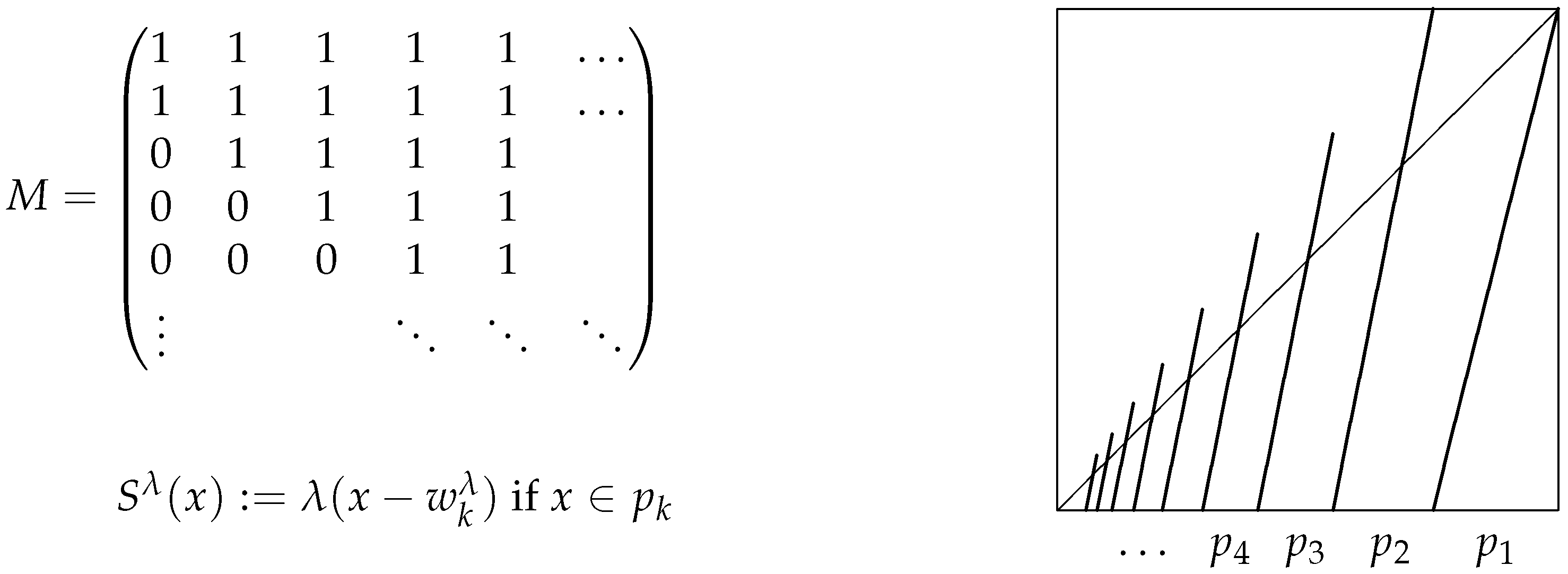
Applying Proposition 2, we associate with $\mathcal{P}$ the transition matrix:

$$M=M(T)={(m_{ij})}_{i,j\in \mathcal{P}}=\left(\begin{array}{ccccc}1& 1+2a_1& 1+2a_2& 1+2a_3& \cdots \\ 1& 0& 0& 0& \dots \\ 0& 1& 0& & \\ ⋮& 0& \ddots & \ddots \end{array}\right)$$

and also (see Figure 2) the corresponding strongly-connected directed graph $G=G(M)$:

In particular, the number of loops of length n from $i_0$ to itself is $f_{00}(n)=1+2a_{n-1}$.

We use the Rometechnique from [21] (see also [22] (Section 9.3)) to compute the entropy of this graph: it is the leading root of the equation:

$$z=1+\sum _{n\ge 1}(1+2a_n)z^{-n}$$

(53)

If we divide this equation by z, then we get:

$$1=z^{-1}+\sum _{n\ge 1}(1+2a_n)z^{-(n+1)}=\sum _{n\ge 1}{f}_{00}(n)z^{-n}$$

From Table 1, it follows that the graph G (the matrix M, the map T) is recurrent for any choice of a sequence ${(a_n)}_{n\ge 0}$ and corresponding finite $\lambda >0$. Proposition 8 and comparing Equations (52) and (53), we find that $e^{h_{top}(T)}={\lambda }_M=\lambda$.

By Remark 5, the map T is of the operator type if and only if ${sup}_n{a}_n<\infty$. In this case, by Table 1 and Proposition 8, ${\Phi }_{00}=1>1/2\ge R=1/{\lambda }_M$, so the corresponding map is always strongly recurrent. For the choice $a_n=a^n$ for some fixed integer $a\ge 2$, the map T is of the non-operator type. In this case, ${\sum }_{n\ge 1}{f}_{00}(n)a^{-n}=\infty$, so $e^{-h_{top}(T)}=1/{\lambda }_M=R<a^{-1}={\Phi }_{00}$; hence, by Table 1, the map T is still strongly recurrent.

We can also take $a_n=a^{n-{\psi }_n}$ for some sublinearly-growing integer sequence ${({\psi }_n)}_{n\ge 1}$ chosen, such that (53) holds for $z=a$, i.e., $a=1+{\sum }_{n\ge 1}{a}^{-n}+2a^{-{\psi }_n}$. In this case, ${\Phi }_{00}=R$ and ${\sum }_n{f}_{00}^{(n)}{R}^n=1$, and the system is null-recurrent or weakly recurrent (not strongly recurrent) depending on whether ${\sum }_{n}n{a}^{-{\psi }_n}$ is infinite or finite.

7.2.3. Transient Non-Operator Example from [23]

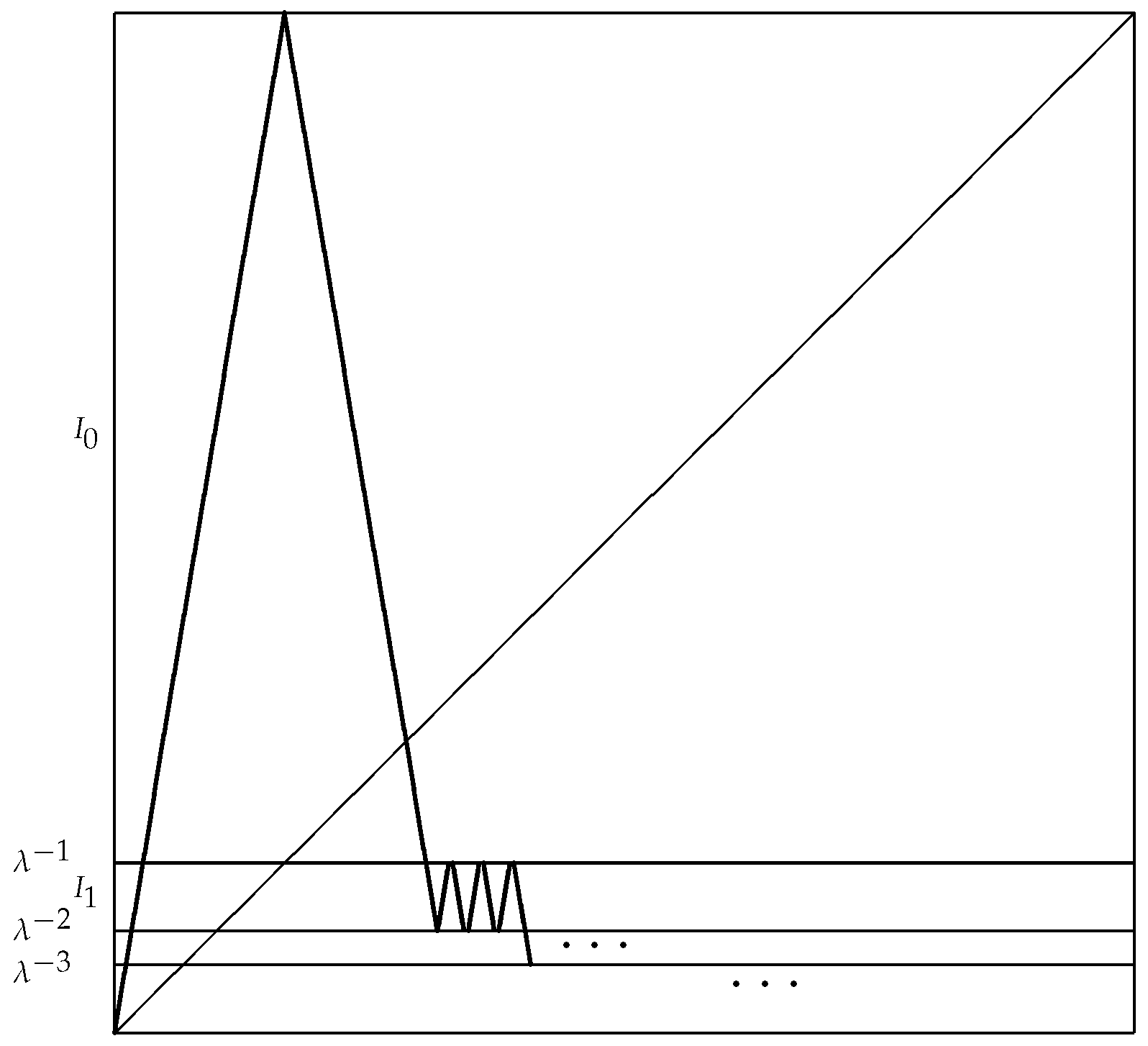
Although up to now, all of our main results have been formulated and proven in the context of continuous maps, many statements remain true also for countably piecewise monotone Markov interval maps that are countably piecewise continuous (this example can be made continuous by replacing each branch with a tent-map of the same height. The λ will be twice as large, and the entropy increases accordingly in that case). We will present a countably-piecewise continuous, countably-piecewise monotone example adapted from [23], where it is studied in detail for its thermodynamic properties.

Let ${(w_k)}_{k\ge 0}$ be a strictly-decreasing sequence in $[0,1]$ with $w_0=1$ and ${lim}_k{w}_k=0$. We will consider the partition $\mathcal{P}={\left\{p_k\right\}}_{k\in \mathbb{N}}$, where the interval map T (see Figure 3) is designed to be linear increasing on each interval $p_k=[w_k,w_{k-1})$ for $k\ge 2$, $p_1=[w_1,w_0]$, $T(p_k)={\bigcup }_{i\ge k-1}{p}_i$ for $k\ge 2$ and $T(p_1)=[0,1]$. With a slight modification of our definition from Section 2, $\mathcal{P}$ is a Markov partition for T, and T is leo. Let $M=M(T)$ be the matrix corresponding to $\mathcal{P}$; see below. In order to have constant slope λ, we need to solve the recursive relation:

$$\left\{\begin{array}{cc}{w}_{k+1}=w_k-w_{k-1}/\lambda \hfill & \text{for}k\ge 1\hfill \\ w_0=1,w_1=1-1/\lambda \hfill \end{array}\right.$$

The characteristic equation ${\alpha }^2-\alpha +1/\lambda =0$ has real solutions ${\alpha }_{\pm }=\frac{1}{2}(1\pm \sqrt{1-4/\lambda })\in (0,1)$ whenever $\lambda \ge 4$. We obtain the solution:

$$w_k^4=2^{-k}(1+k/2)\text{if}\lambda =4$$

and:

$$w_k^{\lambda }=\frac{1-2/\lambda }{2\sqrt{1-4/\lambda }}{\alpha }_{+}^k+\frac{2\sqrt{1-4/\lambda }-1+2/\lambda }{2\sqrt{1-4/\lambda }}{\alpha }_{-}^k\text{if}\lambda >4$$

It is known that $h_{top}(T)=log4$; hence, by Proposition 8, ${\lambda }_M=4$. If we remove site $p_1$ (i.e., remove the first row and column) from M, the resulting matrix is M again, so strongly-connected directed graph $G=G(M)$ contains its copy as a proper subgraph, and due to Theorem 4(i), M and also T are transient.

Writing $v_k^{\lambda }=\left|p_k\right|=w_{k-1}^{\lambda }-w_k^{\lambda }$, we have found, in accordance with Theorem 5, a positive summable λ-solution of Equation (5) for each $\lambda \ge 4$. Summarizing, the map T is conjugate to a map of constant slope λ whenever $\lambda \ge 4$. T is also linearizable, since $\lambda =4={\lambda }_M=e^{h_{top}(T)}$.

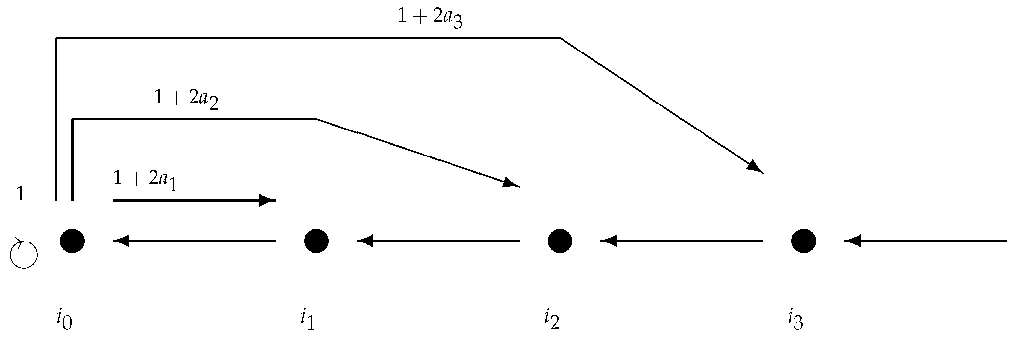
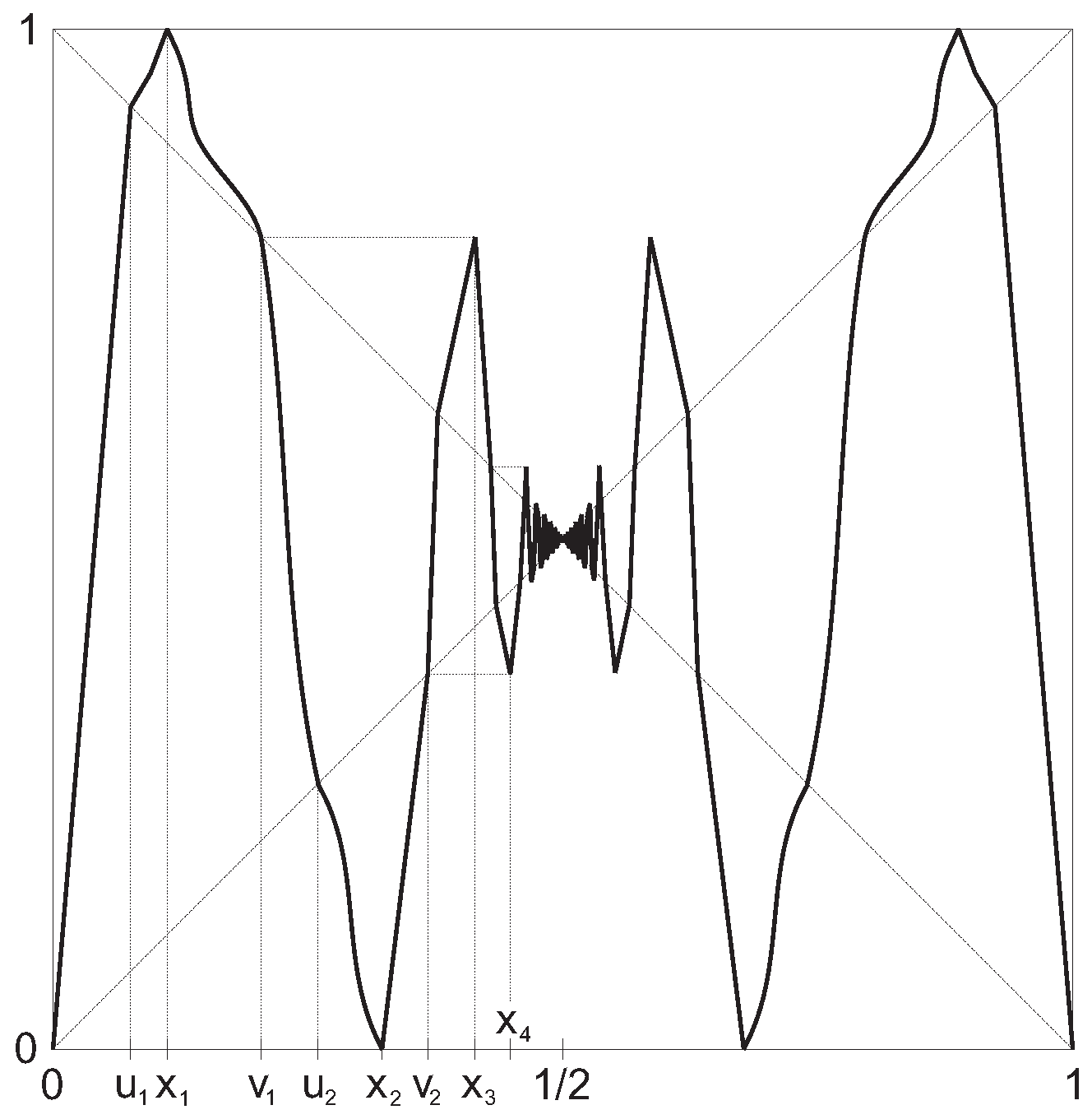
7.2.4. Transient Non-Operator Example from [5]

Let $V={\left\{v_i\right\}}_{i\ge -1}$, $X={\left\{x_i\right\}}_{i\ge 1}$ $V,X$ converge to $1/2$ and $0=v_{-1}=x_0=v_0<x_1<v_1<x_2<v_2<x_3<v_3<\cdots$; the interval map $T=T(V,X):[0,1]\to [0,1]$ satisfies (see Figure 4)

(a)

$T(v_{2i-1})=1-v_{2i-1}$, $i\ge 1$, $T(v_{2i})=v_{2i}$, $i\ge 0$,

(b)

$T(x_{2i-1})=1-v_{2i-3}$, $i\ge 1$, $T(x_{2i})=v_{2i-2},i\ge 1$,

(c)

$T_{u,v}=\left|\frac{T(u)-T(v)}{u-v}\right|>1$ for each interval $[u,v]\subset [x_i,x_{i+1}]$,

(d)

$T(1/2)=1/2$ and $T(t)=T(1-t)$ for each $t\in [1/2,1]$.

Property (c) holds for our $V,X$, since by (a), (b), we have $T_{x_i,x_{i+1}}>2$ for each $i\ge 0$.

Let us denote $\mathcal{F}(V,X)$ the set of all continuous interval maps fulfilling (a)–(d) for a fixed pair $V,X$, and put $\mathcal{F}:={\bigcup }_{V,X}\mathcal{F}(V,X)$. It was shown in [5] that:

• $\mathcal{F}$ is a conjugacy class of maps in $\mathcal{C}\mathcal{P}\mathcal{M}\mathcal{M}$.
• Strongly-connected directed graph $G=G(M)$ contains its copy as a proper subgraph [5] (Theorem 4.5, Figure 3), so due to Theorem 4(i), T is transient.
• The common topological entropy equals $log9$.
• Equation (5) has a positive summable λ-solution for each $\lambda \ge 9=e^{h_{top}(T)}$.

We can factor out the left-right symmetry of this map by using the semi-conjugacy $h(x)=2|x-\frac{1}{2}|$, and the factor map $\tilde{T}$ has transition matrix:

$$M=\left(\begin{array}{cccccc}4& 4& 4& 4& 4& \dots \\ 1& 4& 4& 4& 4& \dots \\ 0& 1& 4& 4& 4& \\ 0& 0& 1& 4& 4& \\ 0& 0& 0& 1& 4& \\ ⋮& & & \ddots & \ddots & \ddots \end{array}\right)$$

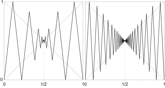
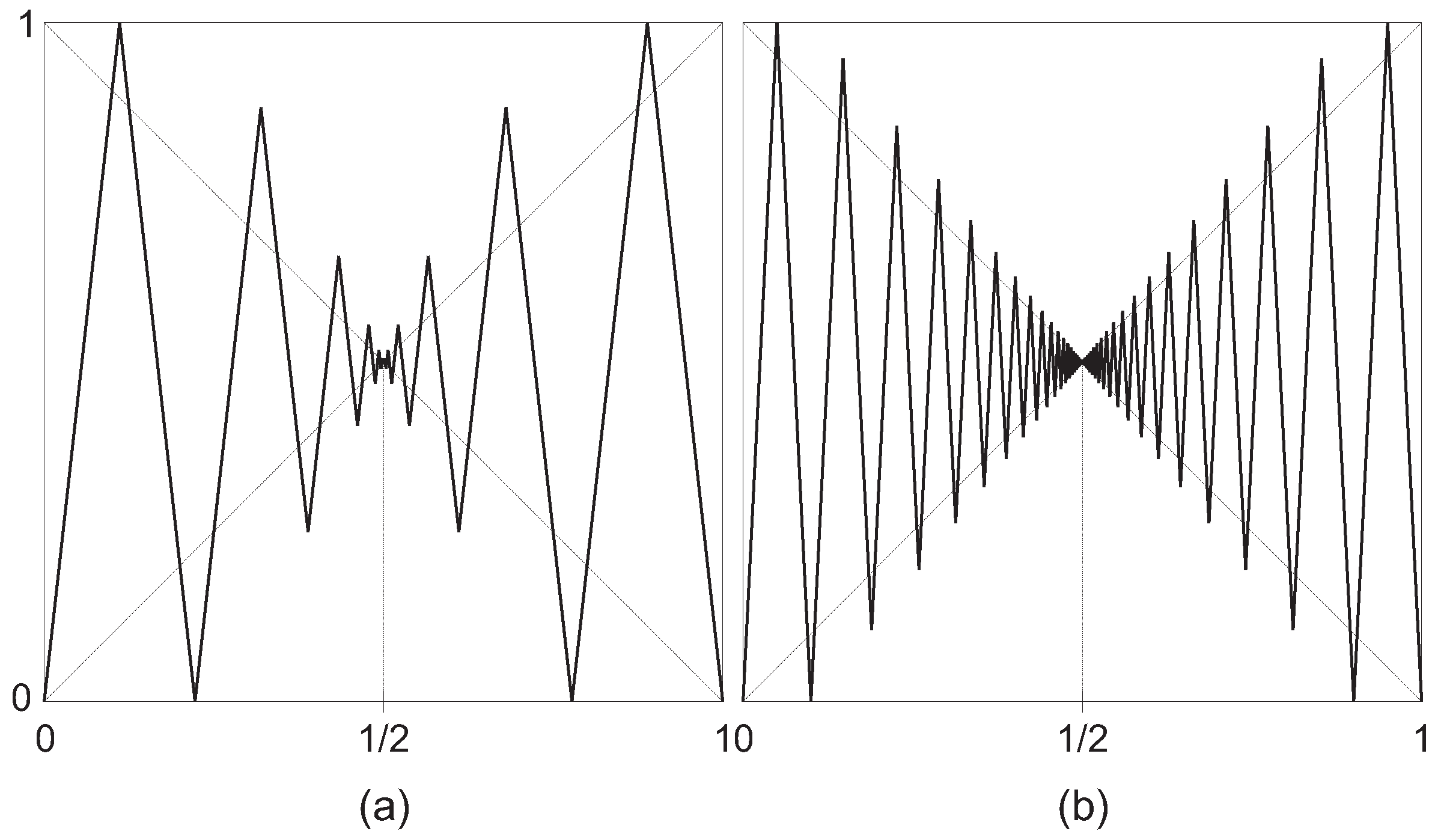
with similar properties as the previous example. Therefore, T is conjugate to a map of constant slope λ whenever $\lambda \ge 9$ (see Figure 5), and also linearizable, since $\lambda =9={\lambda }_M=e^{h_{top}(T)}$.

7.3. One Application of Our Results

Using Proposition 13 let $K=2M(1,1)+E$. We have discussed the fact that K is a transition matrix of a non-leo map $T\in \mathcal{C}\mathcal{P}\mathcal{M}\mathcal{M}$ with corresponding Markov partition denoted by $\mathcal{P}$. Clearly, by Remark 5, K represents a bounded linear operator, denoted it by $\mathcal{K}$, on ${\ell }^1(\mathcal{P})$, so T is of the operator type. We can conclude that:

(i)

${\lambda }_K=5=e^{h_{top}(T)}$, Propositions 8 and 13.

(ii)

${\lambda }_K=r_{\mathcal{K}}=\parallel \mathcal{K}\parallel$, Proposition 13, Section 2, and Equation (3).

(iii)

T is not conjugate to a map of constant slope (is not linearizable), Proposition 13.

(iv)

T is null recurrent, Proposition 13.

(v)

Let ${\mathcal{P}}^{\prime }$ be a Markov partition for T; denote $K^{\prime }$ the transition matrix of T with respect to ${\mathcal{P}}^{\prime }$ representing a bounded linear operator ${\mathcal{K}}^{\prime }$ on ${\ell }^1({\mathcal{P}}^{\prime })$. Since:

$$\forall y\in (0,1):\#T^{-1}(y)=5$$

we have ${\lambda }_{K^{\prime }}=r_{{\mathcal{K}}^{\prime }}=5$; see (i), Section 2 and Proposition 8. Then, by Theorem 11, any recurrent centralized (operator/non-operator) perturbation of T is linearizable. In particular, it is true for any local window perturbation of T on some element of ${\mathcal{P}}^{\prime }$, Proposition 11(i).

(vi)

Let ${\mathcal{P}}^{\prime }$ be a Markov partition for T, which equals $\mathcal{P}$ outside of some interval $[a,b]\subset (0,1)$. Let $T^{\prime }$ be a local window perturbation of T on some element of ${\mathcal{P}}^{\prime }$; from the previous Paragraph (v), it follows that $T^{\prime }$ is strongly recurrent and linearizable. Consider a centralized (operator/non-operator) perturbation $T^{″}$ of $T^{\prime }$ on some ${\mathcal{P}}^{\prime \prime }\subset {\mathcal{P}}^{\prime }$. Then, if $T^{″}$ is recurrent, it is linearizable by Theorem 10. Otherwise, we can use either Theorem 8 (an operator case) or Theorem 9 (non-operator case; $S(j,{\mathcal{P}}^{\prime })$ is finite for $j\in {\mathcal{P}}^{\prime }$) to show that a local window perturbation of $T^{″}$ of a sufficiently large order is linearizable.

References

- Milnor, J.; Thurston, W. On iterated maps of the interval. In Dynamical Systems, Lecture Notes in Math; Springer: Berlin/Heidelberg, Germany, 1988; Volume 1342, pp. 465–563. [Google Scholar]
- Parry, W. Symbolic dynamics and transformations of the unit interval. Trans. Am. Math. Soc. 1966, 122, 368–378. [Google Scholar] [CrossRef]
- Misiurewicz, M.; Szlenk, W. Entropy of piecewise monotone mappings. Stud. Math. 1988, 67, 45–63. [Google Scholar]
- Misiurewicz, M.; Raith, P. Strict inequalities for the entropy of transitive piecewise monotone maps. Discret. Contin. Dyn. Syst. 2005, 13, 451–468. [Google Scholar]
- Bobok, J.; Soukenka, M. On piecewise affine interval maps with countably many laps. Discret. Contin. Dyn. Syst. 2011, 31, 753–762. [Google Scholar] [CrossRef]
- Katok, A.; Hasselblatt, B. Introduction to the Modern Theory of Dynamical Systems; Cambridge University Press: Cambridge, UK, 1995. [Google Scholar]
- Vere-Jones, D. Ergodic properties of non-negative matrices. I. Pac. J. Math. 1967, 22, 361–385. [Google Scholar] [CrossRef]
- Ruette, S. On the Vere-Jones classification and existence of maximal measures for countable topological Markov chains. Pac. J. Math. 2003, 209, 366–380. [Google Scholar] [CrossRef]
- Bobok, J. Semiconjugacy to a map of a constant slope. Stud. Math. 2012, 208, 213–228. [Google Scholar] [CrossRef]
- Alsedá, L.; Llibre, J.; Misiurewicz, M. Combinatorial Dynamics and the Entropy in Dimension One, 2nd ed.; World Scientific: Singapore, Singapore, 2000. [Google Scholar]
- Misiurewicz, M.; Roth, S. Constant slope maps on the extended real line. 2016; arXiv:1603.04198. [Google Scholar]
- Walters, P. An Introduction to Ergodic Theory; Springer: Berlin/Heidelberg, Germany, 1982. [Google Scholar]
- Gurevič, B.M. Topological entropy for denumerable Markov chains. Soviet Math. Dokl. 1969, 10, 911–915. [Google Scholar]
- Salama, I. Topological entropy and recurrence of countable chains. Pac. J. Math. 1988, 134, 325–341. [Google Scholar] [CrossRef]
- Pruitt, W.E. Eigenvalues of non-negative matrices. Ann. Math. Stat. 1964, 35, 1797–1800. [Google Scholar] [CrossRef]
- Chung, K.L. Markov Chains with Stationary Transition Probabilities; Springer: Berlin/Heidelberg, Germany, 1960. [Google Scholar]
- Misiurewicz, M. Horseshoes for mappings of an interval. Bull. Acad. Pol. Sci. 1979, 27, 167–169. [Google Scholar]
- Bobok, J. Strictly ergodic patterns and entropy for interval maps. Acta Math. Univ. Comen. 2003, 72, 111–118. [Google Scholar]
- Taylor, A.E.; Lay, D.C. Introduction to Fuctional Analysis, 2nd ed.; Robert, E., Ed.; Krieger Publishing Company: Malabar, FL, USA, 1980. [Google Scholar]
- Misiurewicz, M.; Roth, S. No semiconjugacy to a map of constant slope. Ergod. Theory Dyn. Syst. 2016, 36, 875–889. [Google Scholar] [CrossRef]
- Block, L.; Guckenheimer, J.; Misiurewicz, M.; Young, L.-S. Periodic points and topological entropy of one-dimensional maps. In Global Theory of Dynamical Systems; Springer: Berlin/Heidelberg, Germany, 1980; Volume 819, pp. 18–34. [Google Scholar]
- Brucks, K.; Bruin, H. Topics from One-Dimensional Dynamics (London Mathematical Society Student Texts); Cambridge University Press: Cambridge, UK, 2004; Volume 62. [Google Scholar]
- Bruin, H.; Todd, M. Transience and thermodynamic formalism for infinitely branched interval maps. J. Lond. Math. Soc. 2012, 86, 171–194. [Google Scholar] [CrossRef]
Figure 1.
The map .
Figure 2.
The Markov graph of ; indicates the number of edges in G from to .
Figure 3.
The transition matrix (left) and graph (right) of the map
Figure 4.
The leo map .
Figure 5.
is conjugate to a map with slope 9 (a) and slope 20 (b).