Nonlinear Thermodynamic Analysis and Optimization of a Carnot Engine Cycle

Abstract

As part of the efforts to unify the various branches of Irreversible Thermodynamics, the proposed work reconsiders the approach of the Carnot engine taking into account the finite physical dimensions (heat transfer conductances) and the finite speed of the piston. The models introduce the irreversibility of the engine by two methods involving different constraints. The first method introduces the irreversibility by a so-called irreversibility ratio in the entropy balance applied to the cycle, while in the second method it is emphasized by the entropy generation rate. Various forms of heat transfer laws are analyzed, but most of the results are given for the case of the linear law. Also, individual cases are studied and reported in order to provide a simple analytical form of the results. The engine model developed allowed a formal optimization using the calculus of variations.

1. Introduction

The oldest and simplest model of a thermo-mechanical engine is due to Carnot [1]. This model supposes two thermal reservoirs of infinite capacity (thermostats) at the source and sink, that implies constant temperatures T_SH (source) and T_SL (sink).

The thermal balance and the entropy balance equations applied to the reversible Carnot direct cycle allow finding the classical result, generally called “Carnot cycle efficiency”. This efficiency corresponds to the upper limit of a thermo-mechanical engine efficiency, named First Law efficiency, that is defined as:

$${\mathsf{\eta }}_I=\frac{mechanicalworkoutput}{energyconsumption}$$

Thus, one recalls the result known as the Carnot cycle efficiency:

$${\mathsf{\eta }}_C=1-\frac{T_{SL}}{T_{SH}}$$

(1)

It is often believed that the Carnot model that relies on Equilibrium Thermodynamics was firstly reconsidered by Curzon and Ahlborn [2], which is not quite precise. Nevertheless, the Finite Time Thermodynamics (FTT) proposes to examine the operation of an endoreversible engine in contact with two thermostats. In this case, the transfer irreversibility appears by the temperature differences at the hot-end and cold-end of the engine (see Figure 1a), respectively, ΔT_H = T_SH − T_H, ΔT_L = T_SL − T_L.

The configuration of the reversible Carnot engine is optimized with respect to the mechanical work or power output. Thus, the expression of the First Law efficiency results, corresponding to maximum of work or power output as:

$${\mathsf{\eta }}_I\left(MAX\left|W\right|\right)=1-\sqrt{\frac{T_{SL}}{T_{SH}}}$$

(2)

This result has been previously obtained by Novikov [4]. Hence it corresponds to what one may call the Carnot–Novikov–Curzon–Ahlborn engine. Equation (2) is often named “nice radical”.

A complementary scheme was established in the same time by Chambadal [5,6]. The assumption of a steady-state regime of a finite sensible heat source was applied, the source being characterized by a heat rate capacity ${\dot{C}}_{SH}={\dot{m}}_{SH}\cdot c_{p_{SH}}$, with ${\dot{m}}_{SH}$-mass flow rate of the source fluid, $c_{p_{SH}}$-mass specific heat at constant pressure assumed independent of temperature. For a perfect heat transfer process to which an effectiveness of the hot-side heat exchanger ε_H = 1 corresponds, the heat rate capacity ${\dot{C}}_{SH}$ provides the maximum heat transfer rate to the endoreversible Carnot engine:

$${\dot{Q}}_H={\dot{C}}_{SH}\left(T_{HSi}-T_H\right)$$

(3)

where T_HSi is the inlet temperature of the source fluid in the hot-end heat exchanger.

The maximum power output of the thermo-mechanical converter is easily obtained [5,6] for the case when considering the sink as thermostat, namely, when T_L = T_SL (perfect thermal contact at sink). The efficiency associated to maximum power output arises as:

$${\mathsf{\eta }}_I\left(MAX\left|\dot{W}\right|\right)=1-\sqrt{\frac{T_{SL}}{T_{SHi}}}$$

(4)

One recalls here that the hot source is characterized by a finite heat capacity rate ${\dot{C}}_{SH}$.

Other complementary results were recently obtained [7,8,9,10,11] and also older works dedicated to this subject were discovered [12].

By using the method of irreversibility ratio [13] instead of the entropy analysis approach, the efficiency corresponding to maximum mechanical work output of the irreversible Carnot engine becomes:

$${\mathsf{\eta }}_I\left(MAX\left|\dot{W}\right|\right)=1-\sqrt{I\frac{T_{SL}}{T_{SH}}}$$

(5)

with I = ΔS_L/ΔS_H (see Figure 1b).

Another alternative to the Finite Time Thermodynamics is the Finite Speed Thermodynamics (FST) proposed by Petrescu and Costea. Reference [14] reports a complete synthesis in this domain. Also, results relative to irreversible Carnot cycle analysis in the frame of FST provide a corrected expression of the “nice radical” as a function of the piston speed, correlations between the maximum cycle efficiency and the entropy generation rate, or maximum power output/efficiency, and the piston speed [15,16,17].

This paper proposes reconsidering the Carnot engine approach by taking into account the finite physical dimensions. Heat transfer conductances and areas in regard to the finite speed of the piston, will be particularly considered.

An overview of the possible objective functions aims to give an idea of the complexity of the optimization problem involving as constraints finite temperature difference at source and sink and finite dimensions (heat conductances or areas) of the heat exchangers. However, only two of the listed objective functions will be discussed hereinafter, namely, maximum power output and minimum entropy generation rate.

By using the sequential optimization method, a three-step optimization is achieved corresponding to progressive consideration of different constraints. Hence, the modeling allowed to provide optimum temperatures of the working gas at the hot-end and cold-end of the engine, optimal allocation of heat transfer areas and optimum characteristic speed of the system associated to these objective functions.

Also, it will be shown (which is for the first time, to our knowledge) how the optimization of the heat exchanger finite surfaces is connected to the characteristic speed of the engine and to the energy dissipation, which also depends on the speed.

A fundamental equation is proposed showing the optimal connection between temperatures at the source and sink, irreversibilities of the converter, and characteristic speed, as well as the link to the system size. It is illustrated in a study case, leading to an analytical solution. These original results are discussed and the consequences are shown, as well as the extensions of this work.

2. Materials and Methods

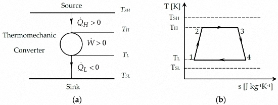
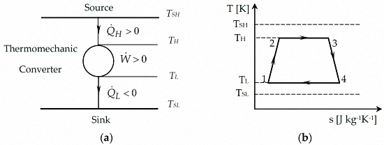
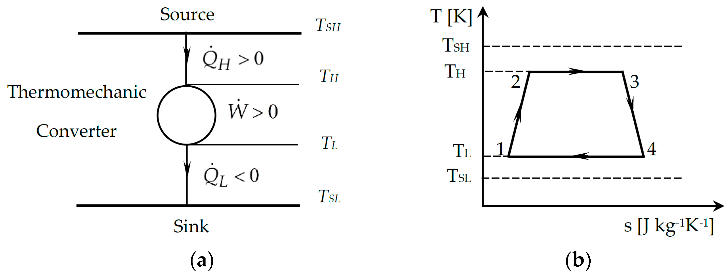
2.1. Model of Carnot Cycle Engine

Although the case of the reverse cycle machines could be simultaneously approached, it seems preferable to limit the reported study to the case of direct cycles for reasons of results accessibility and demonstrations clarity.

An irreversible engine (converter) is considered characterized by irreversible heat transfer at the contact with the source SH or sink SL.

The source and sink are modeled as thermostats with constant temperatures T_SH at the hot-end respectively, T_SL at the cold-end.

The study is reported in the stationary dynamic operating regime so that the converter receives the heat flow ${\dot{Q}}_H$ > 0 from the source and rejects to the sink the heat flow ${\dot{Q}}_L$ < 0, then it produces mechanical power $\dot{W}$ > 0 (see Figure 1a).

The group of source–converter–sink is assumed without any heat loss (adiabatic system).

The energy balance equation of the engine is given by:

$$\dot{W}={\dot{Q}}_H+{\dot{Q}}_L$$

(6)

The First Law efficiency of the engine is expressed as:

$${\mathsf{\eta }}_I=\frac{\dot{W}}{{\dot{Q}}_H}$$

(7)

2.2. Optimization of the CNCA Machine by Using the Entropic Ratio Method

2.2.1. Optimization General Approach

The ratio method is especially used in Finite Speed Thermodynamics and Direct Method [14], which commonly express the mechanical work of any thermal piston machine as:

$$\mathsf{\delta }{W}_{ir}=P_{m,i}\left(1\pm \frac{aw}{c}\pm \frac{\mathsf{\Delta }{P}_f}{P_{m,i}}\pm \frac{b\mathsf{\Delta }{P}_{thr}}{2P_{m,i}}\right)dV$$

(8)

with sign (+) for compression and sign (−) for expansion processes.

Hence, there are three ratios in Equation (8) that represent dissipative mechanisms accounting for pressure losses due to the finite speed of the piston, friction and throttling of the working fluid [14]. Actually, these losses take into account internal irreversibilities of the engine. They can be expressed as functions of the piston speed, design and operational parameters, respectively, and will be considered in further development of the model.

The step proposed here is a global and generic one since it involves only one ratio, I. This ratio appears in the entropy balance equation in the form (9a) or (9b):

$$\frac{I_H{K}_H\left(T_{SH}-T_H\right)}{T_H}+\frac{K_L\left(T_{SL}-T_L\right)}{T_L}=0$$

(9a)

$$\frac{K_H\left(T_{SH}-T_H\right)}{T_H}+\frac{I_L{K}_L\left(T_{SL}-T_L\right)}{T_L}=0$$

(9b)

Equation (9a) imposes I_H ≥ 1. Equation (9b) imposes I_L ≤ 1.

The case with I_H = I_L = 1 corresponds to an endoreversible system.

Hereinafter, it is chosen to work with the ratio I_H, that can be either a parameter (constant on a certain domain), or a function to be identified [18], or sought using the Direct Method, for example, by assuming degradation mechanisms [15].

Most conventional optimizations for an engine are related to the following objective functions:

$${\mathsf{\eta }}_{II}=\frac{{\mathsf{\eta }}_I}{{\mathsf{\eta }}_{lim}}$$

(10)

In the present study, η_lim is the Carnot cycle efficiency, η_C, given by:

$${\mathsf{\eta }}_C=1-\frac{T_{SL}}{T_{SH}}$$

(11)

Note that generally, η_II is not identical to the exergetic efficiency, η_ex. Actually, η_ex is expressed as:

$${\mathsf{\eta }}_{Ex}=\frac{{\mathsf{\eta }}_I}{1-\frac{T_0}{T_{SH}}}$$

(12)

Thus, it is obvious that η_ex is identical to η_II, if T_SL = T₀. This is often close to reality, except certain cases, as for example CHP (Combined Heat and Power) systems.

To the four preceding objective functions given by Equations (6), (7), (10) and (12), it is possible to add those resulting from the energy triangle that is representative of any system or process (Figure 2). This triangle has on the top the Useful Effect provided by the system as a natural optimization choice, while in the bottom the unavoidable Consumption (energy in our case) and Rejects (energy or pollutants) appear. Obviously, the efficiency is inside the triangle, as it is determined by two of the previous fluxes. Then, the environment has to be mentioned, since the ambient properties (mainly temperature) are accounted for (see Equation (12)).

Any system or process under nominal conditions gives rise to:

• entering fluxes, which are generally called EC, energy or material consumptions; to them OF 5 corresponds, namely MIN EC (here ${\dot{Q}}_H$);
• an useful flux or Useful Effect, UE (here MAX $\dot{W}$)
• rejects, R, that may be recoverable (RR, recyclable waste), but most often pollutants for the Environment (RP, pollutant rejects); accordingly, OF 6 namely MIN (R).

The efficiency of the system is represented by the various efficiencies introduced by dimensionless Equations (7), (10)–(12).

Many other optimization criteria could be considered, including environmental and economic ones [19]. These will not be discussed here.

The presentation is mainly concerned with irreversibility in light of its fundamental importance in Thermodynamics. For the case proposed here, the irreversibility of the converter appears as a ratio, I_H, which is a parameter, depending on the problem (Equation (9a)). For example, I_H = f_I(T_L, T_H).

Hence, Equation (9a) acts as a constraint (C1) between natural intensive variables of the problem T_L, T_H. The choice of an objective function (OF) of these variables T_L, T_H (control variables), with C1 as constraint, provides one degree of freedom (DF) leading to the sequential optimization [6]. In this case, K_H, K_L, T_SH, T_SL are parameters (imposed) of the study, i.e., they appear in OF 6 and constraint, C1.

Furthermore, the objective function, OF 7, can be added. It is related to I_SH, for which the minimum, min I_SH, will be sought. Note that I_SH represents the entropy ratio of the studied system and, therefore, it satisfies the system entropy balance equation:

$$\frac{I_{SH}{K}_H\left(T_{SH}-T_H\right)}{T_{SH}}+\frac{K_L\left(T_{SL}-T_L\right)}{T_{SL}}=0$$

(13)

This general optimization approach has reviewed several possible objective functions of the optimization procedure among which only two will be further discussed, namely, maximum power output, OF 1, and minimum entropy production, OF 7.

2.2.2. Particular Results for the Objective Functions MAX $\dot{W}$, MIN I_SH

Maximization of the Power Output of CNCA Engine

Supposing that I_SH = f(T_H, T_L), the Lagrangian function of the optimization can be expressed from Equations (6) and (9a) as follows:

$$L_1\left(T_H,T_L\right)=K_H\left(T_{SH}-T_H\right)+K_L\left(T_{SL}-T_L\right)+\mathsf{\lambda }\left[\frac{f_I\left(T_H,T_L\right)\cdot K_H\left(T_{SH}-T_H\right)}{T_H}+\frac{K_L\left(T_{SL}-T_L\right)}{T_L}\right]$$

(14)

The necessary condition for the optimum is derived as:

$$\left(f_{I,H}-\frac{K_H}{K_L}{f}_{I,L}\right)\frac{T_{SH}-T_H}{T_H}-f_I\frac{T_{SH}}{T_H{}^2}=-\frac{T_{SL}}{T_L{}^2}$$

(15)

This system of two equations with two unknowns needs numerical resolution to get T_H, T_L corresponding to the general case.

Remark 1. 

The function, I_SH = f(T_H, T_L), could be expressed by using FST that is able to provide the entropy generation as a function of the piston speed and temperatures. This improvement makes part of further development of the modeling.

In the present approach, the particular case involves f_I = I = ct, $f_{I,H}=\frac{\partial f_I}{\partial T_H}=0=f_{I,L}=\frac{\partial f_I}{\partial T_L}$. Then simple analytical calculations provide:

$$T_H{}^{*}=\sqrt{I{T}_{SH}}\frac{K_H\sqrt{I{T}_{SH}}+K_L\sqrt{T_{SL}}}{I{K}_H+K_L}$$

(16)

$$T_L{}^{*}=\sqrt{T_{SL}}\frac{K_H\sqrt{I{T}_{SH}}+K_L\sqrt{T_{SL}}}{I{K}_H+K_L}$$

(17)

leading to:

$${\dot{W}}^{*}=MAX\dot{W}=\frac{K_H{K}_L}{I{K}_H+K_L}{\left[\sqrt{T_{SH}}-\sqrt{I{T}_{SL}}\right]}^2$$

(18)

$$I_{SH}\left({\dot{W}}^{*}\right)=\sqrt{I\frac{T_{SH}}{T_{SL}}}$$

(19)

$${\mathsf{\eta }}_I\left({\dot{W}}^{*}\right)=1-\sqrt{I\frac{T_{SL}}{T_{SH}}}$$

(20)

Equation (19) shows that the entropy ratio is an increasing function of the converter irreversibility, the minimum ratio of the system being imposed by the temperatures of the thermostats.

Contrarily, the efficiency corresponding to maximum power (Equation (20)) is a decreasing function of the converter irreversibility. Equation (18) appears as a function of the conductances, K_H and K_L.

Taking account of the finite dimension of the conductances K_H and K_L as a constraint C2 that imposes:

$$K_H+K_L=K_T$$

(21)

one can find by a second sequential optimization that the second order maximum of $\dot{W}$ is associated to Lagrangian L₂(K_H, K_L):

$$L_2\left(T_H,T_L\right)=\frac{K_H{K}_L}{I{K}_H+K_L}{\left(\sqrt{T_{SH}}-\sqrt{I{T}_{SL}}\right)}^2+\mathsf{\lambda }\left[K_H+K_L-K_T\right]$$

(22)

Some calculations will lead to the next analytical results:

$$K_H{}^{*}=\frac{K_T}{1+\sqrt{I}}$$

(23)

$$K_L{}^{*}=\frac{K_T\sqrt{I}}{1+\sqrt{I}}$$

(24)

$$T_H{}^{*}=\sqrt{I{T}_{SH}}\frac{\sqrt{T_{SH}}+\sqrt{T_{SL}}}{1+\sqrt{I}}$$

(25)

$$T_L{}^{*}=\sqrt{T_{SL}}\frac{\sqrt{T_{SH}}+\sqrt{T_{SL}}}{1+\sqrt{I}}$$

(26)

Consequently, Equation (18) becomes:

$$MAX\left(MAX{\dot{W}}^{*}\right)=K_T\frac{{\left(\sqrt{T_{SH}}-\sqrt{I{T}_{SL}}\right)}^2}{{\left(1+\sqrt{I}\right)}^2}$$

(27)

Note that Equations (19) and (20) are not affected by this second optimization. The second order maximum of $\dot{W}$ is an increasing function of the size of the system by K_T, of the temperature difference (T_SH–T_SL), but a decreasing function of the irreversibility, I. The result associated with the endoreversible engine is found.

Consideration of System Irreversibility

Equation (27) shows that the maximum power of the system is obtained for the endoreversible converter, but as it has been seen (Equation (19)), the irreversibility ratio of the system, I_SH, integrates the irreversibility of the converter by the term, $\sqrt{I}$ (internal irreversibility), and the irreversibility associated with heat transfer, through $\sqrt{T_{SH}/T_{SL}}$. Both ratios are greater than 1, but yet different.

• Condition of transfer entropies equipartition

It is proposed here to study the flow of entropy produced at the hot-end, cold-end, and inside the system. Firstly, it is necessary to clearly differentiate the entropy of transit at the hot-end of the converter, and the entropy of transit at the cold-end compared to the converter entropy generation. Actually, the heat transfer rate at the hot-end can be written as:

$${\dot{Q}}_H=T_{SH}\cdot {\dot{S}}_{SH}=T_H\cdot {\dot{S}}_H$$

(28)

Then the entropy production rate due to heat transfer from the source to the converter, ${\dot{S}}_{iH}$, results as:

$${\dot{S}}_{iH}={\dot{S}}_H-{\dot{S}}_{SH}={\dot{Q}}_H\left(\frac{1}{T_H}-\frac{1}{T_{SH}}\right)$$

(29)

The transposition of the reasoning from the converter to the cold-end leads to:

$${\dot{Q}}_L=T_{SL}\cdot {\dot{S}}_{SL}=T_L\cdot {\dot{S}}_L$$

(30)

$${\dot{S}}_{iL}={\dot{Q}}_L\left(\frac{1}{T_L}-\frac{1}{T_{SL}}\right)$$

(31)

By combining Equations (9a), (28) and (29) one gets

$$I_H{\dot{S}}_H+{\dot{S}}_L=0$$

(32)

Equation (32) proves that ${\dot{S}}_H$ ≤ ${\dot{S}}_L$, hence there is no equipartition of transit entropies at the two ends of the converter, except for the endoreversible case (trivial).

Remark 2. 

The equipartition of entropy [20,21] emerged from the linear thermodynamics of the irreversible processes approach when the various fluxes are taken as linear functions of the driving forces. On these bases, structural properties of the optimized processes are established.

However, the entropy production distribution between source and sink provided by the optimization procedure should be analyzed in connection with the model assumptions, as this may differ with their change.

For the particular case of the linear heat transfer law, the expressions of ${\dot{S}}_{iH}$ and ${\dot{S}}_{iL}$ result as follows:

$${\dot{S}}_{iH}=K_H\frac{{\left(T_{SH}-T_H\right)}^2}{T_{SH}{T}_H}$$

(33)

$${\dot{S}}_{iL}=K_L\frac{{\left(T_{SL}-T_L\right)}^2}{T_{SL}{T}_L}$$

(34)

The equipartition of the transfer entropies in the general case involves equality of Equations (33) and (34) under the condition (9a), leading to a system of two equations with two unknowns to be solved:

$$\frac{T_H}{T_{SH}}=1+I\frac{T_L}{T_{SL}}$$

(35)

$$\frac{T_{SH}}{T_H}=1+\frac{K_L}{I{K}_H}\left(1-\frac{T_{SL}}{T_L}\right)$$

(36)

There is a physical solution to the problem in the endoreversible case:

$$T_{Leq}=T_{SL}\frac{1+\frac{K_L}{K_H}+\sqrt{{\left(\frac{K_L}{K_H}\right)}^2-1}}{1+\frac{K_L}{K_H}}$$

(37)

This solution also makes T_{L eq} = T_SL (T_{H eq} = T_SH), which is equivalent to the total reversibility condition (equilibrium thermodynamics).

Note that T_{L eq}, T_{H eq}, T_H, T_L are values of temperatures at transfer entropies equipartition.

• Minimization of the entropy production rate of the system

The entropy production rate in the system is expressed as:

$${\dot{S}}_{iS}={\dot{S}}_{SL}-{\dot{S}}_{SH}$$

(38)

By using Equations (28) and (30) one gets:

$${\dot{S}}_{iS}=\frac{\left|{\dot{Q}}_L\right|}{T_{SL}}-\frac{{\dot{Q}}_H}{T_{SH}}$$

(39)

In the case of the linear heat transfer law, Equation (39) is written:

$${\dot{S}}_{iS}=\frac{K_L\left(T_L-T_{SL}\right)}{T_{SL}}-\frac{K_H\left(T_{SH}-T_H\right)}{T_{SH}}$$

(40)

The optimization considering the objective function OF 7, ${\dot{S}}_{iS}$, given by Equation (40), is always subject to the constraint, C1 (Equation (9a)). The Lagrangian results as:

$$L_3\left(T_H,T_L\right)=\frac{K_L\left(T_L-T_{SL}\right)}{T_{SL}}-\frac{K_H\left(T_{SH}-T_H\right)}{T_{SH}}+\mathsf{\lambda }\left[\frac{f_I\left(T_H,T_L\right)\cdot K_H\left(T_{SH}-T_H\right)}{T_H}+\frac{K_L\left(T_{SL}-T_L\right)}{T_L}\right]$$

(41)

Problem solving requires a system of two equations with two unknowns, T_H, T_L. In the particular case where I_H = I = constant, we find that the condition minimizing the system entropy production rate is the thermodynamic equilibrium, whatever K_H, K_L are. Hence, ${\dot{S}}_{iS}$ is an increasing function of T_L and a decreasing one of T_H. One finds a result obtained for the particular case of a thermoelectric system [22].

2.3. Optimization of the CNCA Machine by Using the Entropy Production Rate Method

2.3.1. General Statement of the Optimization

This entropy production rate method has been preferred in our research for a long time because it is considered appropriate to the identification of an entropy generation function $\dot{S}$ relative to the whole or only a part of the system or process (which is the case in Section “Consideration on System Irreversibility”). Also, it can lead to particular expressions of functions $\dot{S}$ by dissipation mechanisms models, thus joining the Direct Method previously cited [14].

Again, the most comprehensive method is adopted, so that the entropy balance equation of the converter will get a unique form that is equivalent to Equation (9a) or (9b):

$$\frac{{\dot{Q}}_H}{T_H}+\frac{{\dot{Q}}_L}{T_L}+{\dot{S}}_C=0$$

(42)

By preserving the same assumptions as above, namely, linear heat transfer laws, the energy balance equation given by Equation (6) remains the same. The constraint given by the entropy balance equation of the converter becomes:

$$\frac{K_H\left(T_{SH}-T_H\right)}{T_H}+\frac{K_L\left(T_{SL}-T_L\right)}{T_L}+{\dot{S}}_C=0$$

(43)

Actually, it has been shown that ${\dot{S}}_C$ is a function of T_H, T_L. Moreover, it also depends on the characteristic speed of the system, w. This was experimentally confirmed for reverse cycle machines (heat pumps) [21], and it should also apply to engines.

• Entropy production rate of the converter

The entropy production rate of the converter is generally denoted as:

$${\dot{S}}_C=f_C\left(T_H,T_L,w\right)$$

(44)

The simplest mathematical forms of Equation (44) that can be used are:

-

${\dot{S}}_C=\dot{S}=cte$ ($\dot{S}=0$, endoreversible)

-

${\dot{S}}_C=S\text{'}\left(T_H-T_L\right)$ (linear dependence on temperature difference)

-

${\dot{S}}_C=C\cdot ln\frac{T_H}{T_L}$ (logarithmic dependence on temperature ratio)

Experiments done on heat pumps have shown that the coupling to the speed is made by the linear law through S', such that:

$$S^{\text{'}}={\dot{S}}_0+{\dot{S}}_0^{\text{'}}\cdot w$$

(45)

• Heat transfer laws at the source and sink

The most commonly used heat transfer law is the linear one, expressed as:

$${\dot{Q}}_i=K_i\left(T_{Si}-T_i\right)(i=H\mathrm{or}L)$$

The conductances, K_i, were supposed constant in Section 2.2, where they were introduced. A step further in the development of a more general model is based on the fact that the literature provides correlations expressed as:

$$K_i=A_i{f}_i\left(T_i,w\right)$$

(46)

Therefore, the functions f_i from Equation (46) could be identified as nonlinear heat transfer laws, namely:

• generalized convective heat transfer law [23,24]

  $${\dot{Q}}_i=K_i{\left(T_{Si}-T_i\right)}^n$$

  (47)
• generalized radiative heat transfer law [25,26]

  $${\dot{Q}}_i=K_i\left(T_{Si}^n-T_i^n\right)$$

  (48)

  with K_i—generalized conductances.

2.3.2. General and Required Condition for the Existence of Optimum Corresponding to MAX $\dot{W}$

The Lagrangian function leading to the maximization of the power output of the engine L₄ (T_H, T_L, w) is composed as follows:

$$\begin{array}{l}{L}_4\left(T_H,T_L,w\right)=A_H{f}_H\left(T_H,w\right)\left(T_{SH}-T_H\right)+A_L{f}_L\left(T_L,w\right)\left(T_{SL}-T_L\right)+\\ +\mathsf{\lambda }\left[\frac{A_H{f}_H\left(T_{SH}-T_H\right)}{T_H}+\frac{A_L{f}_L\left(T_L,w\right)\left(T_{SL}-T_L\right)}{T_L}+f_C\left(T_{H,}{T}_L,w\right)\right]\end{array}$$

(49)

There are three variables (T_H, T_L, w) for one constraint, thus the model has two independent variables (2 degrees of freedom).

The system of three equations to be solved is studied in the particular case where the dependence of K_H, K_L on temperature is negligible, so that f_H(T_H, w) = f_H(w); f_L(T_L, w) = f_L(w). Furthermore, if one supposes identical modes of heat transfer to the hot- and cold-ends, it comes:

$$f_H\left(w\right)=f_L\left(w\right)=f\left(w\right)$$

(50)

This corresponds to the particular case of the dominant convective heat transfer laws (not radiative, nor conductive).

In the particular case of convective heat transfer laws of the Newton type (linear) satisfying the condition (50) and a linearized law of the converter energy dissipation rate settled by Equation (44) [27], it results:

$$f_C\left(T_H,T_L,w\right)=S_C\left(w\right)\left(T_H-T_L\right)$$

(51)

In the sequential optimization relative to the control variables, T_H, T_L, the following required condition is derived:

$$\frac{T_{SH}}{T_H{}^2}-\frac{S_C\left(w\right)}{k_H\left(w\right)A_H}=\frac{T_{SL}}{T_L{}^2}+\frac{S_C\left(w\right)}{k_L\left(w\right)A_L}={\mathsf{\alpha }}^2$$

(52)

$$k_H{A}_H\frac{T_{SH}-T_H}{T_H}+k_L{A}_L\frac{T_{SL}-T_L}{T_L}+S_C\left(w\right)\left(T_H-T_L\right)=0$$

(53)

Note that in Equation (52) the variables can be separated. Therefore, by considering the intermediate variable, α, the resolution is reduced to a second order equation as following:

$${\mathsf{\alpha }}^2\left(k_H{A}_H\sqrt{T_{SH}}+k_L{A}_L\sqrt{T_{SL}}\right)-\mathsf{\alpha }\left(k_H{A}_H+k_L{A}_L\right)+2S_C\left(\sqrt{T_{SH}}-\sqrt{T_{SL}}\right)=0$$

(54)

Equation (54) can be numerically solved, except for the endoreversible case.

As the purpose here is not to present a complete solution, but the existence of an extensive combined solution, the results are illustrated in the case close to endoreversibility.

2.3.3. Sequential Optimization of the Engine Power Output

Asymptotic Solution for the Case S_C(w) Smaller than k_HA_H and k_LA_L

For this case one gets:

$${\mathsf{\alpha }}_{\lim }=\frac{k_H{A}_H+k_L{A}_L}{k_H{A}_H\sqrt{T_{SH}}+k_L{A}_L\sqrt{T_{SL}}}-2S_C\frac{\sqrt{T_{SH}}-\sqrt{T_{SL}}}{k_H{A}_H+k_L{A}_L}$$

(55)

Furthermore, the maximum power output of the engine is derived:

$$MA{X}_1\left|\dot{W}\right|=\frac{k_H{A}_H{k}_L{A}_L}{k_H{A}_H+k_L{A}_L}[{\left(\sqrt{T_{SH}}-\sqrt{T_{SL}}\right)}^2-\frac{2S_C\left(T_{SH}-T_{SL}\right){\left(k_H{A}_H\sqrt{T_{SH}}+k_L{A}_L\sqrt{T_{SL}}\right)}^3}{k_H{A}_H{k}_L{A}_L{\left(k_H{A}_H+k_L{A}_L\right)}^2}]$$

(56)

The power output of the engine expressed by Equation (56) depends on k_H, k_L, A_H, A_L, S_C, T_SH, T_SL, which are parameters. Optimum temperatures, T_H^*, T_L^*,are obtained by the asymptotic forms of the following expressions:

$$T_H{}^{*}=\frac{\sqrt{T_{SH}}}{\sqrt{{\mathsf{\alpha }}^2+\frac{S_C}{k_H{A}_H}}}$$

(57)

$$T_L{}^{*}=\frac{\sqrt{T_{SL}}}{\sqrt{{\mathsf{\alpha }}^2+\frac{S_C}{k_L{A}_L}}}$$

(58)

Optimization of the Physical Geometric Dimensions A_H, A_L, of the System

The heat transfer areas, A_H, A_L, are considered as variables, subject to a constraint of finite dimensions given by the A_T parameter. The optimization aims to find the optimal distribution of the heat transfer area between the hot- and cold-ends of the system:

$$A_H+A_L=A_T$$

(59)

Remark 3. 

Apparently, Equations (21) and (59) provide similar finite dimension constraints for the optimization problem. However, they are quite different from the optimal conditions yielded from the optimization procedure. Besides, the finite constraint on heat conductances is simpler and less precise but gives easier analytical results. Thus, both of them are important in the optimization modeling.

The variational calculus allows to find a solution close to the limit and improvable by iteration, such as:

$$A_H{}^{*}=A_T\frac{\sqrt{k_L}}{\sqrt{k_H}+\sqrt{k_L}}-\frac{S}{2k_H{k}_L{A}_T{}^2}$$

(60)

$$A_L{}^{*}=A_T\frac{\sqrt{k_H}}{\sqrt{k_H}+\sqrt{k_L}}+\frac{S}{2k_H{k}_L{A}_T{}^2}$$

(61)

with

$$S=6S_C\left(w\right)\left(\sqrt{T_{SH}}+\sqrt{T_{SL}}\right){\left(\frac{k_H{A}_H\sqrt{T_{SH}}+k_L{A}_L\sqrt{T_{SL}}}{k_H{A}_H+k_L{A}_L}\right)}^2{A}_T$$

(62)

Then, by assuming the formal symmetry of the heat transfer laws (k_H(w)= k_L(w) = k(w)) and by limiting S_C(w) to the first order form, the expression of the maximum power MAX₂ $\left|\dot{W}\right|$ in the limiting case results:

$$MA{X}_2\left|\dot{W}\right|=\frac{k\left(w\right)}{4}{A}_T{\left(\sqrt{T_{SH}}-\sqrt{T_{SL}}\right)}^2-\frac{S_C\left(w\right)}{4}\left(T_{SH}-T_{SL}\right){\left(\sqrt{T_{SH}}+\sqrt{T_{SL}}\right)}^3$$

(63)

Knowing that $\frac{\partial k}{\partial w}=k_{,w}$ and $\frac{\partial S_C}{\partial w}=S_{C,w}$ are positive, Equation (64) proves by derivation with respect to w that there exists an optimum power with respect to a characteristic speed of the system, w. It results w*, the optimum characteristic speed that satisfies the equation:

$$\frac{\partial k}{\partial w}=\frac{1}{A_T}{\left(\sqrt{T_{SH}}+\sqrt{T_{SL}}\right)}^3\frac{\partial S_C}{\partial w}$$

(64)

This fundamental equation is obtained for the first time to our knowledge. It shows the optimal connection between heat transfers to the source and sink, with the irreversibilities of the converter, as well as the link to the system size (A_T) and temperatures at the source and sink (T_SH, T_SL).

3. Discussion—Partial Conclusion

The particular forms of Equation (64) provide some interesting trends that are discussed hereafter.

Note that in the case of purely convective heat transfers, k(w) takes the general form:

$$k\left(w\right)=k^{\text{'}}{w}^n$$

(65)

(a)

For a dissipation law, similar to that reported in [18], Equation (51) becomes:

$$S_C\left(w\right)=S_{Co}+S_C^{\text{'}}\cdot w$$

(66)

Then, from Equation (64), the optimum speed can be expressed as:

$$w^{*}=\sqrt[n-1]{\frac{S_C^{\text{'}}{\left(\sqrt{T_{SH}}+\sqrt{T_{SL}}\right)}^3}{n{k}^{\text{'}}{A}_T}}$$

(67)

Remark 4. 

Generally, the value of n is close to 3, according to the correlations indicated in the literature and Dulong–Petit, a law mainly used by Angulo Brown’s group [23,24], for which Equation (68) yields:

$$w^{*}=\sqrt{\frac{S_C^{\text{'}}\left(\sqrt{T_{SH}}+\sqrt{T_{SL}}\right)}{3k^{\text{'}}{A}_T}}\left(\sqrt{T_{SH}}+\sqrt{T_{SL}}\right)$$

Therefore, it is known that w* increases with both T_SH and T_SL, as well as with the ratio S_C'/k', but decreases with A_T. Small machines have larger optimum speeds.

(b)

For a dissipation law as an mth power function of the speed:

$$S_C\left(w\right)=S^{\text{'}}\cdot w^m$$

(68)

Equation (64) leads to the following expression of the optimum speed:

$$w^{*}=\sqrt[n-m]{\frac{m}{n}\frac{S^{\text{'}}}{k^{\text{'}}}\frac{{\left(\sqrt{T_{SH}}+\sqrt{T_{SL}}\right)}^3}{A_T}}$$

(69)

Therefore, there is a confirmation of the trends identified on Equation (67). Note that the irreversibility function (Equation (68)) satisfies the Second Law of Thermodynamics since the entropy flux vanishes at zero speed (corresponding to a quasi-static process that is characteristic to the Equilibrium Thermodynamics).

Equation (66) that was obtained by identification to experiments can only be a particular relationship, valid in a speed-limited physical domain. However, it accounts well for the irreversibility associated with temperature differences between input and output of the converter (T_H–T_L).

It is assumed that a more comprehensive relationship must exist to account for all of irreversibility coupled mechanisms (including ∆P with mass transfers).

4. Extensions—Particular Results

4.1. Optimization Statement on an Entropic Base

This approach differs a little from the previous one (Section 2.3). It is based on the following fundamental relationship:

$${\dot{S}}_i=\frac{{\dot{Q}}_i}{T_i}=K_i\left(w\right)\frac{T_{Si}-T_i}{T_i}$$

(70)

Relation (66) preserves the heat transfer assumption used in Section 2.2 and Section 2.3.

Note that here, ${\dot{S}}_i$ is the entropy rate associated with transit (or transfer) processes, not the entropy production rate, as it will be seen below. The shaping is almost identical to previous approaches, except that in the calculations, a factor, a(w), appears in Equations (57) and (58) such that:

$$a\left(w\right)=\frac{S_C\left(w\right)}{K\left(w\right)}$$

(71)

This arises from the variable conductance reasoning, K(w), and not transfer coefficient, k(w), but with the assumption of equipartition of transfer conductances (K_H(w) = K_L(w) = K(w)).

Then the resolution leads to an asymptotic solution:

$${\mathsf{\alpha }}_{\lim }=\frac{2}{\sqrt{T_{SH}}+\sqrt{T_{SL}}}-\frac{3a}{4}\left(\sqrt{T_{SH}}-\sqrt{T_{SL}}\right)$$

(72)

and it results for MAX $\left|\dot{W}\right|$:

$$MA{X}_1\left|\dot{W}\right|=\frac{K\left(w\right)}{2}{\left(\sqrt{T_{SH}}-\sqrt{T_{SL}}\right)}^2-\frac{S_C\left(w\right)}{16}\left(T_{SH}-T_{SL}\right)\cdot \left[4\left(T_{SH}+T_{SL}\right)+{\left(\sqrt{T_{SH}}+\sqrt{T_{SL}}\right)}^2\right]$$

(73)

This asymptotic solution confirms the results obtained in Section “Optimization of the Physical Geometric Dimensions A_H, A_L, of the System” and also the observed trends, in addition to the existence of an optimal characteristic speed providing maximum engine power in the presence of irreversibility.

4.2. Particularization to Calculate the Various Entropy Production Rates

To illustrate the results, the case of the endoreversible engine (${\dot{S}}_C$ = 0) is chosen, with K_H and K_L parameters. One finds analytically:

$${\mathsf{\alpha }}_{opt}=\frac{K_H+K_L}{K_H\sqrt{T_{SH}}+K_L\sqrt{T_{SL}}}$$

(74)

The temperatures corresponding to the optimum power of engine result as:

$$T_H{}^{*}=\sqrt{T_{SH}}\frac{K_H\sqrt{T_{SH}}+K_L\sqrt{T_{SL}}}{K_H+K_L}$$

(75)

$$T_L{}^{*}=\sqrt{T_{SL}}\frac{K_H\sqrt{T_{SH}}+K_L\sqrt{T_{SL}}}{K_H+K_L}$$

(76)

and the maximum power of the endoreversible engine is:

$$MA{X}_1{\left|\dot{W}\right|}_{endo}=\frac{K_H{K}_L}{K_H+K_L}{\left(\sqrt{T_{SH}}-\sqrt{T_{SL}}\right)}^2$$

(77)

Then, it is easy to show that when variable conductances fulfilling the condition K_H + K_L = K_T are considered, equipartition of conductances leads to maximum power, expressed by:

$$MA{X}_2{\left|\dot{W}\right|}_{endo}=\frac{K_T}{4}{\left(\sqrt{T_{SH}}-\sqrt{T_{SL}}\right)}^2$$

(78)

This result is in full agreement with that one deduced from Equation (63). It also allows to examine the distribution of the entropy production rates in the most favorable case (endoreversible). Hence, the entropy production rate at the hot-end is:

$${\dot{S}}_{i{H}_{endo}}=K_H\frac{{\left(T_{SH}-T_H{}^{*}\right)}^2}{T_{SH}\cdot T_H{}^{*}}=\frac{K_H{K}_L{}^2}{K_H+K_L}\frac{{\left(\sqrt{T_{SH}}-\sqrt{T_{SL}}\right)}^2}{\left(K_H\sqrt{T_{SH}}+K_L\sqrt{T_{SL}}\right)\sqrt{T_{SH}}}$$

(79)

The entropy production rate at the cold-end of the endoreversible engine is:

$${\dot{S}}_{i{L}_{endo}}=K_L\frac{{\left(T_{SL}-T_L{}^{*}\right)}^2}{T_{SL}\cdot T_L{}^{*}}=\frac{K_L{K}_H{}^2}{K_H+K_L}\frac{{\left(\sqrt{T_{SH}}-\sqrt{T_{SL}}\right)}^2}{\left(K_H\sqrt{T_{SH}}+K_L\sqrt{T_{SL}}\right)\sqrt{T_{SL}}}$$

(80)

Concluding, equipartition of the entropy production of heat transfer processes can be encountered only if:

$$\frac{K_L}{\sqrt{T_{SH}}}=\frac{K_H}{\sqrt{T_{SL}}}$$

(81)

On the other side, the total entropy production rate of the endoreversible engine, ${\dot{S}}_{iT}$ corresponds to:

$${\dot{S}}_{iT}={\dot{S}}_{iH}+{\dot{S}}_{iL}$$

(82)

Then, one easily finds using the Equations (79), (80) and (82):

$${\dot{S}}_{iT}=\frac{K_H{K}_L}{K_H+K_L}\frac{{\left(\sqrt{T_{SH}}-\sqrt{T_{SL}}\right)}^2}{\sqrt{T_{SH}}\sqrt{T_{SL}}}$$

(83)

This expression shows that when K_H + K_L = K_T (finite physical dimensions constraint), the total entropy production rate of the endoreversible engine passes through a maximum for equipartition of heat transfer conductances (K_H = K_L = K_T/2).

Thereby, one can conclude that for the endoreversible engine the equipartition of heat transfer conductances corresponds to the maximum mechanical power of the engine, and also to the maximum entropy production rate. This confirms other works’ results [7,22,28,29,30,31] and shows that the entropy generation minimization (EGM) recommended in quite an important number of works [32,33,34] does not have the character of generality we would like to give it. It was widely used in the 1990’s as a powerful optimization tool. For some particular constraints, the optimization results have shown equipartition of heat transfer conductances associated with maximum power output. Actually, the results can be completely different when the constraints associated with an objective function are changed. Thus it is necessary to properly raise the issue. Generally, the minimum entropy generation rate is associated with high values of or maximum efficiency (if it exists) or to an economical operation regime of the system.

The incidence of converter irreversibilities affects the results more. Other variables, like the characteristic speed, w, can further modify the results (Section 2.3.2).

5. Conclusions

This work provides models of the irreversible Carnot engine with finite dimensions (heat transfer conductances or surfaces, characteristic speed of the engine), and local description of the engine irreversibilities through (1) the entropy ratio method of irreversibility and (2) the method of entropy production rate. The aim of the study was to develop the models by considering the engine irreversibility introduced by the two methods, to prove that they can provide optimal regimes and to derive analytical results, at least for particular cases.

Even if a general approach is proposed by the formal optimization based on the variational calculus, the objective functions are focused on the maximum power output of the engine and the minimum entropy production rate in steady state operation conditions.

The method of sequential optimization used in the modeling allowed to obtain the temperatures associated to optimum (T_H*, T_L*), afterwards the optimal allocation of heat transfer areas (A_H*, A_L*), and finally w*, the engine speed at the optimum operation point. The main findings related to maximizing the engine power extend previous results reported in the literature. Thus, a new generalized form of the nice radical has been proposed in the paper.

The models proposed herein also allow to demonstrate the relationship between the physical dimensions of the system (T_i, K_i, A_i) and a characteristic speed of the engine for the first time, to our knowledge. This connection appears highly nonlinear owing to the coupling dimension-speed. The asymptotic behavior near the endoreversibility can provide meaningful analysis results corresponding to realistic tendencies. Primarily, there is an optimum speed associated with the best compromise between transfer and conversion of energy.

Another important conclusion is obtained through the analysis of the associated entropy production rate. Regardless of the method used to characterize the irreversibility (entropy ratio method, or entropy production rate method), the result of the study shows that:

• the maximum power supplied by the engine does not correspond systematically to the minimum entropy production rate;
• equipartition of entropy production rate is not associated to the maximum power delivered by the engine (endoreversible or not).

Therefore, these results open up a new horizon for the future of Engineering Thermodynamics, also from a fundamental thermodynamic point of view.

The further development of modeling regarding the other objective functions considered in the general optimization procedure, the replacement of the entropic ratio used here as a parameter with an expression derived by using FST for the entropy generation rate as a function of the piston speed, as well as the comparison of the two methods (ratio method, or entropy production rate method), is in progress.

References and Notes

1. Carnot, S. Réflexion Sur la Puissance Motrice du Feu et Des Machines Propres à Développer Cette Puissance; Albert Blanchard: Paris, France, 1953. (In French) [Google Scholar]
2. Curzon, F.L.; Ahlborn, B. Efficiency of a Carnot Engine at Maximum Power Conditions. Am. J. Phys. 1975, 43, 22–24. [Google Scholar] [CrossRef]
3. Feidt, M.; Université de Lorraine, Nancy, France. Personal Communication, 23 February 2013.
4. Novikov, I.I. The efficiency of Atomic Power Stations (a review). J. Nucl. Energy 1958, 7, 125–128. [Google Scholar] [CrossRef]
5. Chambadal, P. Les Centrales Nucléaires; Armand Colin: Paris, France, 1957. (In French) [Google Scholar]
6. Chambadal, P. Evolutions et Applications du Concept D’entropie; Dunod: Paris, France, 1963; p. 84. (In French) [Google Scholar]
7. Feidt, M. Thermodynamique Optimale en Dimensions Physiques Finies; Hermes, Lavoisier: Paris, France, 2013. [Google Scholar]
8. Park, H.; Kim, M.S. Thermodynamic performance Analysis of Sequential Carnot Cycles using Heat Sources with Finite Heat Capacity. Energy 2014, 68, 592–598. [Google Scholar] [CrossRef]
9. Mehta, P.; Polkovnikov, A. Efficiency bounds for non-equilibrium heat engines. Ann. Phys. 2012, 332, 110–126. [Google Scholar] [CrossRef]
10. Yu, J.; Zhou, Y.; Liu, Y. Performance Optimization of an Irreversible Carnot Refrigerator with Finite Mass Flow Rate. Int. J. Refrig. 2011, 34, 567–572. [Google Scholar] [CrossRef]
11. Frikha, S.; Abid, M.S. Performance Optimization of an Irreversible Combined Carnot Refrigerator based on Ecological Criterion. Int. J. Refrig. 2016, 65, 153–165. [Google Scholar] [CrossRef]
12. Vaudrey, A.; Lanzetta, F.; Feidt, M. HB reitlinger and the origins of the efficiency at maximum power formula for heat engines. J. Non-Equilib. Thermodyn. 2014, 39, 199–203. [Google Scholar] [CrossRef]
13. Petrescu, S.; Costea, M.; Feidt, M.; Ganea, I.; Boriaru, N. Advanced Irreversible Thermodynamics of Processes with Finite Speed and Finite Dimensions; Editura AGIR: Bucharest, Romania, 2015. [Google Scholar]
14. Petrescu, S.; Costea, M. Development of Thermodynamics with Finite Speed and Direct Method; Editura AGIR: Bucharest, Romania, 2011. [Google Scholar]
15. Petrescu, S.; Harman, C.; Costea, M.; Feidt, M. Thermodynamics with finite speed versus thermodynamics in finite time in the optimization of Carnot cycle. In Proceedings of the 6th ASME-JSME Thermal Engineering Joint Conference, Kohala, HI, USA, 16–20 March 2003.
16. Petrescu, S.; Harman, C.; Bejan, A. The Carnot cycle with external and internal irreversibility. In Proceedings of the Florence World Energy Research Symposium, Energy for The 21st Century: Conversion, Utilization and Environmental Quality, Firenze, Italy, 6–8 July 1994.
17. Petrescu, S.; Feidt, M.; Harman, C.; Costea, M. Optimization of the irreversible Carnot cycle engine for maximum efficiency and maximum power through use of finite speed thermodynamic analysis. In Proceedings of the 15th International Conference on Efficiency, Cost, Optimization, Simulation and Environmental Impact of Energy Systems, ECOS’2002, Berlin, Germany, 3–5 July 2002; Tsatsaronis, G., Moran, M., Cziesla, F., Bruckner, T., Eds.; Volume II, pp. 1361–1368.
18. Petre, C.; Feidt, M.; Costea, M.; Petrescu, S. A model for study and optimization of real-operating refrigeration machines. Int. J. Energy Res. 2009, 33, 173–179. [Google Scholar] [CrossRef]
19. Feidt, M. Energétique: Concepts et Applications; Dunod: Paris, France, 2006. [Google Scholar]
20. Tondeur, D. Optimisation thermodynamique: Équipartition de production d'entropie. Available online: https://hal.archives-ouvertes.fr/hal-00560251/ (accessed on 25 June 2016).
21. Tondeur, D. Optimisation thermodynamique. Equipartition: Exemples et applications. Available online: https://hal.archives-ouvertes.fr/hal-00560257/ (accessed on 25 June 2016).
22. Dong, Y.; El-Bakkali, A.; Feidt, M.; Descombes, G.; Perilhon, C. Association of finite-time thermodynamics and a bond-graph approach for modelling an irreversible heat engine. Entropy 2012, 14, 1234–1258. [Google Scholar] [CrossRef]
23. Ares de Parga, G.; Angulo-Brown, F.; Navarrete-González, T.D. A variational optimization of a finite-time thermal cycle with a nonlinear heat transfer law. Energy 1999, 24, 997–1008. [Google Scholar] [CrossRef]
24. Ramírez-Moreno, M.A.; González-Hernández, S.; Angulo-Brown, F. The role of the Stefan–Boltzmann law in the thermodynamic optimization of an n-Müser engine. Phys. A Stat. Mech. Appl. 2016, 444, 914–921. [Google Scholar] [CrossRef]
25. Qin, X.; Chen, L.; Sun, F.; Wu, C. Performance of an endoreversible four-heat-reservoir absorption heat pump with a generalized heat transfer law. Int. J. Therm. Sci. 2006, 45, 627–633. [Google Scholar] [CrossRef]
26. Song, H.; Chen, L.; Sun, F. Endoreversible heat-engines for maximum power-output with fixed duration and radiative heat-transfer law. Appl. Energy 2007, 84, 374–388. [Google Scholar] [CrossRef]
27. Petre, C. The use of Thermodynamics with Finite Speed to Study and Optimization of Carnot Cycle and Stirling Machines. Ph.D. Thesis, University Henri Poincaré of Nancy and University Politehnica of Bucharest, Bucharest, Romania, 2007. [Google Scholar]
28. Dong, Y.; El-Bakkali, A.; Descombes, G.; Feidt, M.; Perilhon, C. Association of finite-time thermodynamics and a bond-graph approach for modelling an endoreversible heat engine. Entropy 2012, 14, 642–653. [Google Scholar] [CrossRef]
29. Feidt, M.; Costea, M.; Petre, C.; Petrescu, S. Optimization of Direct Carnot Cycle. Appl. Therm. Eng. 2007, 27, 829–839. [Google Scholar] [CrossRef]
30. Feidt, M.; Université de Lorraine, Nancy, France. Private communication, 2014.
31. Haseli, Y. Performance of irreversible heat engines at minimum entropy generation. Appl. Math. Model. 2013, 37, 9810–9817. [Google Scholar] [CrossRef]
32. Bejan, A. Entropy Generation Minimization; CRC Press: Boca Raton, FL, USA, 1996. [Google Scholar]
33. Salamon, P.; Hoffmann, K.H.; Schubert, S.; Berry, R.S. Thermodynamics in finite time. IV: Minimum entropy production in heat engines. Phys. Rev. A 1980, 21, 2115–2129. [Google Scholar] [CrossRef]
34. Johanessen, E.; Kjelstrup, S. Minimum entropy production rate in plug flow reactors: An optimal control problem solved for SO2 oxidation. Energy 2004, 29, 2403–2423. [Google Scholar] [CrossRef]
Figure 1. Carnot–Novikov–Curzon–Ahlborn Machine [3]: (a) scheme; (b) cycle representation in T–s diagram.
Entropy 18 00243 g001
Figure 2. Energy Triangle connecting the Useful Effect (UE), the Energy Consumption (EC) and the Reject (R).
Entropy 18 00243 g002