Maximum Entropy Learning with Deep Belief Networks

Abstract

Conventionally, the maximum likelihood (ML) criterion is applied to train a deep belief network (DBN). We present a maximum entropy (ME) learning algorithm for DBNs, designed specifically to handle limited training data. Maximizing only the entropy of parameters in the DBN allows more effective generalization capability, less bias towards data distributions, and robustness to over-fitting compared to ML learning. Results of text classification and object recognition tasks demonstrate ME-trained DBN outperforms ML-trained DBN when training data is limited.

1. Introduction

Understanding how a nervous system computes requires determining the input, the output, and the transformations necessary to convert the input into the desired output [1]. Artificial neural networks are a conceptual framework that provide insight into how these transformations are carried out, and have also played a crucial factor in the success of many pattern recognition tasks such as for handwriting [2] and object [3] detection. An important feature of neural networks is their ability to capture the underlying regularities in a task domain by representing the input with multiple layers of active neurons. This distributed representation of the input is based on the hierarchal processing and information flow of biological systems [4,5]. In a multi-layered network, complex internal representations can also be constructed by repeatedly adjusting the weights of the connections in order to ensure that the output is close to the desired output [6]. The method of weight adjustment is called ”back-propagation” and is interpreted as a maximum likelihood (ML) procedure if each output is specified by a conditional probability distribution [7]. This learning procedure generalizes correctly to new cases after sufficient training with an external supervisor, however the learning time scales poorly and is not incremental in nature [8]. In contrast, humans learn concepts with richer representations from fewer examples [9,10] and can even generate their own new examples using top-down processing of high-level representations to disambiguate low-level perceptions [11]. Therefore, the long-term goal is to build deep [12] hierarchal structures [13] that are highly flexible [14], efficient to train, and provide generative models that can produce examples with the same probability distribution as the examples it is shown [15].

Recent advances in deep learning have generated much interest in hierarchical generative models such as Deep Belief Networks (DBNs). Although the increased depth of deep neural networks (DNNs) has led to significant performance gains, training becomes difficult where the cost surface is non-convex and high-dimensional with many local minima [16]. Therefore, training is often carried out in two phases to (1) initialize and then (2) fine-tune the weights of deep architectures. The $first$ $phase$ involves greedy layer-wise unsupervised pretraining where each layer of a DBN learns a non-linear transformation of its own input that captures the main variation in its input [17,18,19,20,21]. The DBN is constructed from multi-layers of feature detectors, each characterized by a restricted Boltzmann machine (RBM). Each RBM uses the Contrastive Divergence (CD) [22] approximation of the log-likelihood gradient to accelerate the learning process. By pairing each feed-forward layer with a feed-back layer that reconstructs the input of the layer from its output, the generative model guarantees that most of the information contained in the input is preserved in the output of the layer. After initializing weights, a logistic layer is placed on top to perform discriminative tasks. The $second$ $phase$ involves fine-tuning the combined DBN–DNN with a supervised training criterion for gradient-based optimization of the prediction error. The generative DBN pretraining in the first phase is thought to benefit discriminative DNNs by discovering latent variables [23], providing marginal conditioning [24], disentangling factors of variation [25], optimizing the hidden layers [26], constraining parameter spaces to basins of attraction [16], and providing a regularization mechanism [27] that minimizes variance and introduces a bias towards configurations that are useful for unsupervised learning. The most important conclusion [28] from all of these studies is that DBN pretraining improves robustness compared to random initiation, especially with increasing network depth [24] and at the lower layers of the DNN where the gradient information becomes less informative as it is back-propagated through more layers (referred to as the problem of vanishing gradients [29]).

The present study explores whether the maximum entropy (ME) principle can improve generative DBN architectures for pretraining DNNs. The over-riding principle of ME is that distributions should be as uniform and unbiased as possible when dealing with estimation problems given incomplete knowledge or data [30]. ME probability distributions have been widely reported in both living neural networks and artificial neural networks to account for spatial and temporal correlation structure. When applied to neuronal data, ME models have quantitatively described the activity in biological networks [31], ensembles [32], connectivity matrices [33], spike trains [34], and receptive fields [35]. When applied to artificial neural networks, the ME principle has been explored with source separation [36], associative memory [37], signal reconstruction [38], and energy contrast functions [39]. The ME approach is especially attractive in neural networks since the high parallelism spreads the computational costs over the units to overcome the problems of low speeds and robustness [40,41]. The ME model can also be extended as a weight matrix that directly connects the input and output layers [42], and DNNs were recently considered as an ME classifier in which the feature functions are learned (because learning the parameters in the softmax layer is equivalent to training a conditional ME model on features of the input vector) [43,44]. In this paper, we specifically analyze how ME learning can be further incorporated into deep architectures by expanding on our preliminary DBN pretraining work [45], which was motivated by a seminal study comparing the benefits of latent maximum entropy in a Boltzmann Machine [46].

Traditionally, the ML learning algorithm is used with RBMs and DBNs [47,48] (denoted ML-RBM and ML-DBN hereinafter). The basic principle of the ML method [49] is that the event with the greatest probability is most likely to occur, so parameters should be chosen that maximize the probability of the observed sample data. The ML estimation possesses several attractive properties including: consistency, asymptotic normality, and efficiency when the sample size tends to infinity [50]. However, DNNs that are pretrained with ML-DBNs are prone to be over-trained and mismatched with the test environments [51]. In addition, ML-RBMs provide no guarantees that the features implemented by their hidden layers will be related to the supervised learning task [52]. Furthermore, ML-RBMs can result in overcomplete representations with redundant hidden units [53]. Previous research has addressed the deficiencies of ML-DBNs and ML-RBMs by developing regularization to compensate small perturbations over training samples [51], introducing discriminative components to improve their performance as a classifier [52], adding terms to enforce sparse solutions [54], and even replacing ML-DBNs with ML deep Boltzmann machines (DBMs) [55]. Rather than adhering to ML learning methods, our previous work [45] proposed ME learning for RBMs and DBNs (denoted ME-RBM and ME-DBN hereinafter) as the principle is known to be effective for combining different sources of evidence from complex and unstructured natural systems [56]. Due to the ability to fit the data without making specific assumptions or having to commit extensively to unseen data, we hypothesized that pretraining with generative ME-DBNs would enable the resulting discriminative DNNs to be more unbiased to data distributions and robust to over-fitting issues compared to those pretrained by ML-DBNs. The preliminary results in several object recognition tasks showed ME-DBNs outperformed ML-DBNs, with noticeable gains when the amount of training data was limited. These conclusions were particularly encouraging as it is known that the outcome of discriminative training often relies on the amount of available training data [52], and in many real world applications it is impossible or expensive to collect labeled training data for rebuilding models [57,58,59].

The most difficult problem in building network architectures is discovering parallel organizations that do not require so much problem-dependent information [15], and the ultimate goal of machine learning research is to produce methods that are capable of learning complex behaviors without human intervention or prior knowledge [14]. Moreover, generalization from sparse data is central for human concept-learning [60]. Neural recordings from living neural networks have shown the ME approach uniquely specifies higher-order neuronal correlations in a hierarchical organization [31] by assuming that the best model fits the correlations found in the data up to that particular level and is maximally unconstrained for all higher-order correlations [32]. Likewise, generative DBN models are intended to characterize higher-order correlation properties as each layer captures the complicated and higher-order correlations between the activities of hidden features in the layer below. In fact, our original ME-DBN learning algorithm can be expanded by incorporating constraints [61] such as weight decay and sparsity during the training process (denoted as constrained maximum entropy (CME) for CME-RBM and CME-DBN hereinafter). Since more complex interactions make it less obvious to construct correlation functions which capture the underlying order among neurons in a network [62], the analysis of ME and CME learning in DBNs could provide insight into the multitude of subsystems in the nervous system that acquires, processes, and communicates information to recode the incoming signals into a more efficient form [63]. In this paper, results in both object recognition and text classification demonstrate that DNNs initialized by ME-DBN outperform DNNs initialized by ML-DBN, suggesting ME-DBN provides a better initial starting point for DNN classifiers. Towards the goal of an ”efficient coding hypothesis” [64], we also show the inclusion of weight decay and sparsity constraints in CME-DBNs enhances ME learning even further compared to ML learning when training data is limited.

The rest of this paper is organized as follows: Section 2 introduces the relevant background, Section 3 presents the proposed ME and CME algorithms with derivations and justifications. Section 4 presents the experimental setup and results. Section 5 concludes this work.

2. Preliminaries and Background

This section reviews background related to RBM, DBN, and the proposed ME learning algorithm.

2.1. Restricted Boltzmann Machine

The RBM is an undirected bipartite graphical model whose probability distribution is governed by an energy function, E, with the parameter set $\lambda =\{\mathbf{W},\mathbf{b},\mathbf{c}\}$:

$$E(\mathbf{v},\mathbf{h};\lambda )=-\sum _{i=1}^V{c}_i{v}_i-\sum _{j=1}^H{b}_j{h}_j-\sum _{i=1}^V\sum _{j=1}^H{v}_i{h}_j{w}_{ij},$$

(1)

where $v_i$ and $h_j$ are the binary state of visible unit i and hidden unit j; $c_i$ and $b_j$ are their corresponding biases; $w_{ij}$ is the weight between visible and hidden unit; V and H are the numbers of visible and hidden units, respectively. The bipartite connection of the graph makes it easy to infer the hidden states given the visible states. The joint probability for $\{\mathbf{v},\mathbf{h}\}$ is formulated as follows:

$$p(\mathbf{v},\mathbf{h};\lambda )=\frac{exp(-E(\mathbf{v},\mathbf{h};\lambda \left)\right)}{Z},$$

(2)

where Z is the partition function, $Z={\sum }_{\mathbf{v},\mathbf{h}}exp(-E(\mathbf{v},\mathbf{h};\lambda \left)\right)$, which ensures that the function in Equation (2) is a valid probability function. The conditional probability of the RBM is:

$$\begin{array}{cc}\hfill p\left(v_i\right|\mathbf{h};\lambda )& =sigm(c_i+\sum _{j=1}^H{w}_{ij}{h}_j),\hfill \\ \hfill p\left(h_j\right|\mathbf{v};\lambda )& =sigm(b_j+\sum _{i=1}^V{w}_{ij}{v}_i),\hfill \end{array}$$

(3)

where $sigm(.)$ is the sigmoid function, $sigm\left(x\right)={(1+exp(-x))}^{-1}$. Conventionally, the ML criterion is utilized to compute the parameters in the RBM. The log probability of the training data, given the model parameters, can be derived as follows: $logp(\mathbf{v};\lambda )=log{\sum }_{\mathbf{h}}p(\mathbf{v},\mathbf{h};\lambda )$. Taking the partial derivative of $logp(\mathbf{v};\lambda )$ with respect to the parameter set λ yields

$$\begin{array}{cc}\hfill \frac{\partial logp(\mathbf{v};\lambda )}{\partial \lambda }& =-\sum _{\mathbf{h}}p\left(\mathbf{h}\right|\mathbf{v})\frac{\partial E(\mathbf{v},\mathbf{h};\lambda )}{\partial \lambda }+\sum _{\mathbf{v},\mathbf{h}}p(\mathbf{v},\mathbf{h})\frac{\partial E(\mathbf{v},\mathbf{h};\lambda )}{\partial \lambda }.\hfill \end{array}$$

(4)

From Equation (4), the parameter updating rule becomes:

$$\begin{array}{cc}\hfill w_{ij}^t& =w_{ij}^{t-1}+\eta *(<v_i{h}_j{>}_{data}-<v_i{h}_j{>}_{model}),\hfill \\ \hfill c_i^t& =c_i^{t-1}+\eta *(<v_i{>}_{data}-<v_i{>}_{model}),\hfill \\ \hfill b_j^t& =b_j^{t-1}+\eta *(<h_j{>}_{data}-<h_j{>}_{model}),\hfill \end{array}$$

(5)

where η denotes the step size, $<{>}_{data}$ denotes empirical expectation, and $<{>}_{model}$ denotes expectation with respect to model distribution.

The learning process, given by Equation (5), can be interpreted as follows: to perform parameter learning, the probability that the model assigns to the observed data should be increased (positive phase), whereas the probability of what the model believes should be reduced (negative phase) [15]. The learning process is finished (meaning that the gradient has vanished) when the predictions of what the model believes becomes the same as the observed training data. However, a critical issue of the learning algorithm is that the computation of the expected values of the model parameters is intractable. Even when the Monte Carlo method is used, it still takes a long time to get the Markov chain to mix. To solve this problem, the CD method was proposed to approximate the learning process. In CDk, the negative-phase samples from the model are drawn by alternating Gibbs sampling only k times rather than until equilibrium is reached. Previous studies confirmed CDk provides satisfactory performance [65,66].

2.2. Gaussian Unit RBM for Continuous Data

Equations (1)–(3) can be utilized to estimate model parameters in the RBM when the input is binary data. To model continuous data, the binary visible units can be replaced by linear units with independent Gaussian noise. The energy function in Equation (1) is thus modified as follows:

$$\begin{array}{c}\hfill E(\mathbf{v},\mathbf{h};\lambda )=\frac{1}{2{\sigma }^2}\sum _{i=1}^V{v}_i^2-\frac{1}{{\sigma }^2}(\sum _{i=1}^V{c}_i{v}_i+\sum _{j=1}^H{b}_j{h}_j+\sum _{i=1}^V\sum _{j=1}^H{v}_i{w}_{ij}{h}_j),\end{array}$$

(6)

where σ is the standard deviation of the Gaussian noise. Accordingly, the conditional probabilities become:

$$\begin{array}{cc}\hfill p\left(v_i\right|\mathbf{h};\lambda )& =\mathcal{N}(v_i;c_i+\sum _{j=1}^H{w}_{ij}{h}_j,{\sigma }^2),\hfill \\ \hfill p(h_j=1|\mathbf{v};\lambda )& =sigm\left(\frac{1}{{\sigma }^2}(b_j+\sum _{i=1}^V{w}_{ij}{v}_i)\right),\hfill \end{array}$$

(7)

where $\mathcal{N}(.)$ represents a Gaussian distribution. Since the input data are now modeled using a Gaussian distribution, this RBM is called a Gaussian–Bernoulli RBM [48].

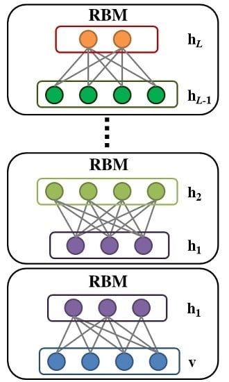
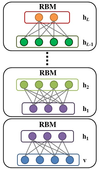
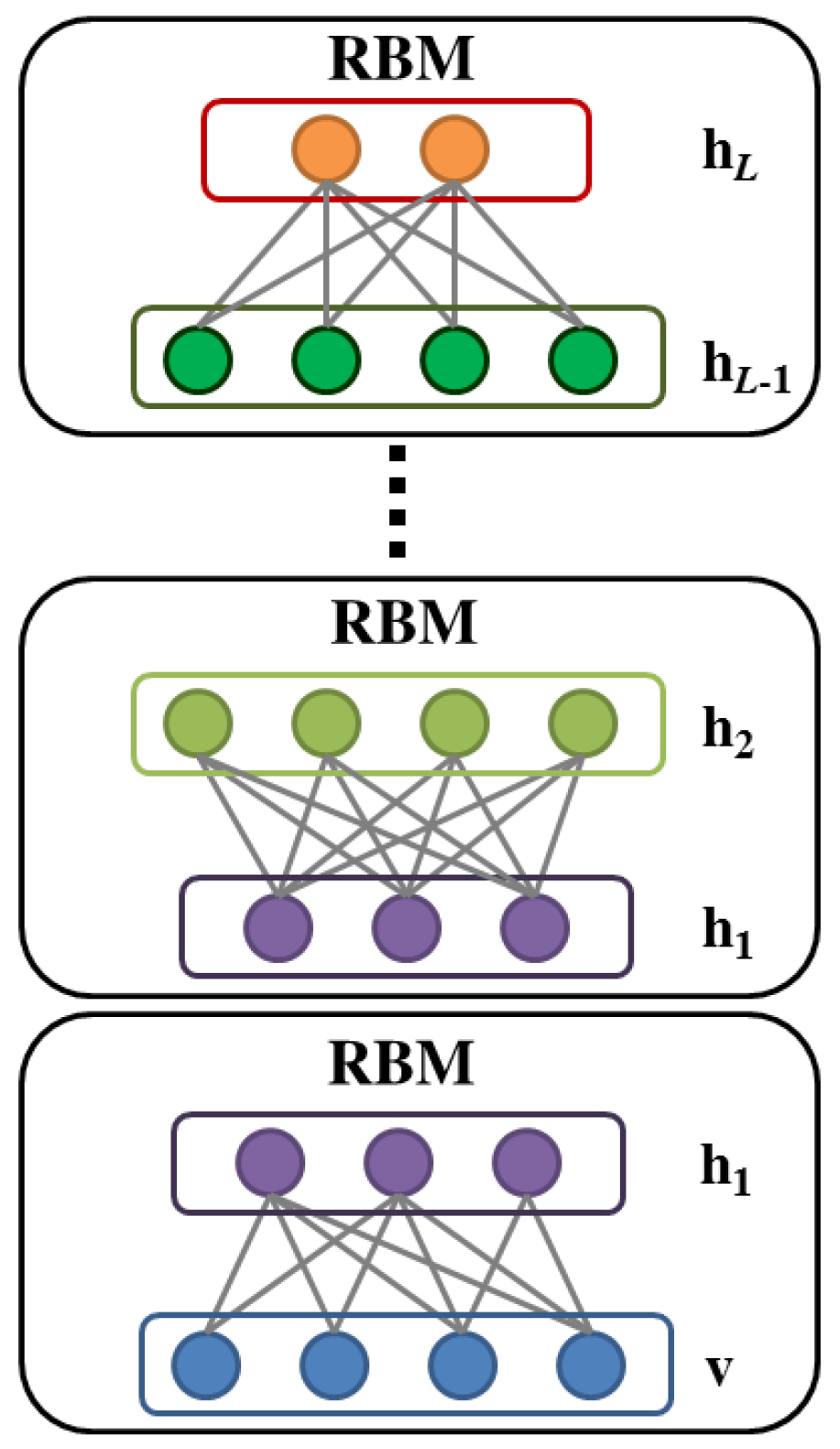
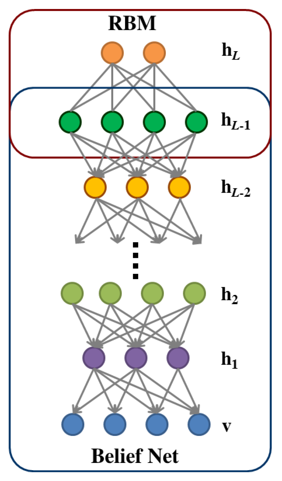
2.3. Deep Belief Network

Figure 1 shows an efficient greedy layer-wise learning procedure developed for training DBNs [18]. The parameters of the first RBM are estimated using the observed training data. In the following layers, the greedy learning algorithm uses the hidden activation of the previous layer as input data to train another RBM. The previous investigation showed that the variational lower bound of data log-likelihood is guaranteed under this greedy layer-wise learning framework, suggesting that stacking another layer of RBM does not reduce the generative power of the model.

A hybrid model is established by stacking up RBMs, as illustrated in Figure 2. The top two layers form the RBM and the lower layers form a directed belief net [16,18]. This hybrid model is called a deep belief network (DBN), whose probability function is given by:

$$\begin{array}{c}\hfill p(\mathbf{v},{\mathbf{h}}_1,{\mathbf{h}}_2,...,{\mathbf{h}}_L)=p({\mathbf{h}}_{L-1},{\mathbf{h}}_L)p\left(\mathbf{v}\right|{\mathbf{h}}_1)\prod _{l=2}^{L-1}p\left({\mathbf{h}}_{l-1}\right|{\mathbf{h}}_l),\end{array}$$

(8)

where L denotes the total number of layers. Now, let $\mathbf{D}=\{{\mathbf{h}}_1,{\mathbf{h}}_2,...,{\mathbf{h}}_L\}$ denote the entire set of hidden layers in the DBN, so we then have

$$\begin{array}{c}\hfill p(\mathbf{v},\mathbf{D})=p(\mathbf{v},{\mathbf{h}}_1,{\mathbf{h}}_2,...,{\mathbf{h}}_L).\end{array}$$

(9)

2.4. Maximum Entropy Learning

ME learning aims to estimate a set of parameters, ${\lambda }^{*}$, which maximizes the entropy of a probabilistic model, $p(x;\lambda )$, where x is a random variable denoting the data:

$$\begin{array}{cc}\hfill {\lambda }^{*}& =arg\underset{\lambda }{max}H\left(\lambda \right)\hfill \\ & =arg\underset{\lambda }{min}\{{\int }_{x}p(x;\lambda )log\left(p(x;\lambda )\right)dx\},\hfill \end{array}$$

(10)

subject to

$$\begin{array}{c}\hfill {\int }_{x}p(x;\lambda )f_r\left(x\right)dx=\sum _{\tilde{x}}p(\tilde{x};\lambda )f_r\left(\tilde{x}\right),r=1,2,...R,\end{array}$$

(11)

where $\tilde{x}$ is the observed training data, $f_r(.)$ denotes the r-th type of feature of a data instance, and R is the number of distinct features. Equation (11) stands for a constraint that the expected sufficient statistics of the model and the data should match. This prevents the learning results in a naive model (uniform distribution). This ME learning criterion has been extensively adopted in the field of natural language processing (NLP) research [61,67,68,69] where the input dimension is the size of a typically large vocabulary. In these cases, the training data is often insufficient for a delicate probabilistic model to be estimated. In previous NLP studies, ME learning exhibited a superior capacity to make the model unbiased with respect to unseen data. Therefore, probabilistic models trained by ME learning can offer a more favorable generalization capacity.

3. Maximum Entropy Deep Belief Network

This section explains the proposed maximum entropy deep belief network (ME-DBN). First, the ME learning criterion is presented for estimating parameters in the RBM. Next, the greedy layer-wise learning method for building a DBN is introduced. Finally, constraint terms are developed to be integrated into the objective function to regularize and encourage the sparsity of DBN model parameters.

3.1. Maximum Entropy Restricted Boltzmann Machine

The objective function of the ME-RBM is formulated as,

$$\begin{array}{cc}\hfill {\lambda }^{*}& =arg\underset{\lambda }{max}H\left(\lambda \right)\hfill \\ & =arg\underset{\lambda }{min}\{\sum _{\mathbf{v},\mathbf{h}}p(\mathbf{v},\mathbf{h};\lambda )logp(\mathbf{v},\mathbf{h};\lambda )\},\hfill \end{array}$$

(12)

subject to

$$\begin{array}{cc}\hfill \sum _{\mathbf{v},\mathbf{h}}p(\mathbf{v},\mathbf{h};\lambda )f\left(\mathbf{v}\right)& =\mu \left(\tilde{\mathbf{v}}\right),\hfill \\ \hfill \sum _{\mathbf{v},\mathbf{h}}p(\mathbf{v},\mathbf{h};\lambda )f\left(\mathbf{h}\right)& =\mu \left(\mathbf{h}\right),\hfill \\ \hfill \sum _{\mathbf{v},\mathbf{h}}p(\mathbf{v},\mathbf{h};\lambda )f(\mathbf{v},\mathbf{h})& =\mu (\tilde{\mathbf{v}},\mathbf{h}),\hfill \end{array}$$

(13)

where we have defined three types of features $f\left(\mathbf{v}\right)$ , $f\left(\mathbf{h}\right)$ , and $f(\mathbf{v},\mathbf{h})$, each corresponding to the activated state of $\mathbf{v}$, $\mathbf{h}$, and $\mathbf{v}{\mathbf{h}}^T$; $\mu \left(\tilde{\mathbf{v}}\right)$, $\mu \left(\mathbf{h}\right)$, and $\mu (\tilde{\mathbf{v}},\mathbf{h})$ correspond to their empirical expectations, which are estimated from the data by

$$\begin{array}{cc}\hfill \mu \left(\tilde{\mathbf{v}}\right)& =\frac{{\sum }_{n=1}^N{\tilde{\mathbf{v}}}^n}{N},\hfill \\ \hfill \mu \left(\mathbf{h}\right)& =\frac{{\sum }_{n=1}^N{\sum }_{\mathbf{h}}p\left(\mathbf{h}\right|{\tilde{\mathbf{v}}}^n;\lambda )\mathbf{h}}{N},\hfill \\ \hfill \mu (\tilde{\mathbf{v}},\mathbf{h})& =\frac{{\sum }_{n=1}^N{\sum }_{\mathbf{h}}p\left(\mathbf{h}\right|{\tilde{\mathbf{v}}}^n;\lambda ){\tilde{\mathbf{v}}}^n{\mathbf{h}}^T}{N},\hfill \end{array}$$

(14)

where ${\tilde{\mathbf{v}}}^n$ is the n-th data sample, N is the number of data samples, and ${(·)}^T$ is the transpose operator. A previous study showed that solving the constrained optimization problem (i.e., Equations (12)–(14)) is equivalent to solving another unconstrained optimization problem [70,71]. Therefore, our problem can be solved by applying the expectation maximization (EM) algorithm:

$$\begin{array}{cc}\hfill {\lambda }^{*}& =arg\underset{\lambda }{max}Q(\lambda ,{\lambda }^{{}^{\prime }}),\hfill \end{array}$$

(15)

where the Q function is the expectation of the complete likelihood (${\sum }_{\mathbf{v}\in \tilde{X}}logp(\mathbf{v},\mathbf{h};\lambda )$):

$$\begin{array}{cc}\hfill Q(\lambda ,{\lambda }^{{}^{\prime }})& =\sum _{\mathbf{v}\in \tilde{X}}\sum _{\mathbf{h}}p\left(\mathbf{h}\right|\mathbf{v};{\lambda }^{{}^{\prime }})logp(\mathbf{v},\mathbf{h};\lambda ),\hfill \end{array}$$

(16)

where $\tilde{X}$ is the whole training set, ${\lambda }^{\prime }$ is the parameter set from the previous iteration.

In the E-step, the expectations of the three features are computed, as defined earlier. In the M-step, the Q function is maximized with respect to the model parameters. The computation of expectations in the E-step is easy for the RBM, while maximizing the Q function in the M-step is intractable. Accordingly, some approximation methods are required. The original estimation of Equations (12)–(14) is not a convex optimization problem because there are latent variables in the model, whereas maximizing the Q function itself is a convex problem. Thus, we can apply either iterative scaling [72,73] or generalized EM [74] along with Monte Carlo approximation to solve the problem. In this study, the generalized EM is used, and the overall learning procedure is demonstrated in Algorithm 1.

Algorithm 1 Expectation Maximization–Contrastive Divergence Algorithm

Input:  With the parameter set $\lambda =\{\mathbf{W},\mathbf{b},\mathbf{c}\}$, we have $p(\mathbf{v},\mathbf{h};\lambda )=\frac{exp(-E(\mathbf{v},\mathbf{h};\lambda \left)\right)}{Z}$ and the energy function E is defined in Equation (1). Initialize:  Let ${\lambda }^{\left(0\right)}=\{\mathbf{W},\mathbf{b},\mathbf{c}\}$ randomly initialized. E-step:  Given the current estimate of ${\lambda }^{\left(t\right)}$, compute the empirical expected value for all features given by Equation (14). M-step:  Maximize the Q function iteratively until $|{\lambda }^{new}-{\lambda }^{old}|<ϵ$, where ϵ is a pre-defined value. For the k-th parameter in λ, namely ${\lambda }_k$, the update is done by performing gradient ascent with $$\begin{array}{c}\hfill \frac{\partial Q}{\partial {\lambda }_k}={\mu }_k-\sum _{\mathbf{v},\mathbf{h}}p(\mathbf{v},\mathbf{h};{\lambda }^{\left(old\right)})\frac{\partial E(\mathbf{v},\mathbf{h};{\lambda }^{\left(old\right)})}{\partial {\lambda }_k},\end{array}$$ where ${\mu }_k$ denotes the empirical expectation of the k-th parameter in λ, which is obtained from Equations (12)–(14). CD is applied to approximate the expectation in the second term. Repeat:  until convergence. Return:  ${\lambda }^{*}$ (the final parameter set).

3.2. Greedy Layer-Wise Learning

For the greedy layer-wise learning of ML-DBN, adding another layer of RBM using previous hidden activations as new data will not reduce the total log-likelihood [16]. When using the ME learning algorithm to estimate a DBN, this justification still holds because each RBM is guaranteed to have data log-likelihood at a locally optimal point. Therefore, the variational bound for likelihood holds, suggesting that stacking another layer of RBM will not reduce the total likelihood. The difference between ME-DBN and ML-DBN is that, among the local optima to be determined, ML-DBN chooses the one with a higher likelihood, whereas ME-DBN chooses the one with a higher entropy [70,71]. Given that the log-likelihood is also locally optimal in ME-DBN, we can use the same argument to conclude that greedy layer-wise learning in ME-DBN still guarantees the variational lower bound on the data log-likelihood. In addition, we can derive

$$\begin{array}{c}\hfill H(\mathbf{v},{\mathbf{h}}_1,{\mathbf{h}}_2)\ge H(\mathbf{v},{\mathbf{h}}_1),\end{array}$$

(17)

where the inequality holds by the property of entropy ($H(a,b,c)\ge H(a,b)$ for any random variable ($a,b,c$). Therefore, whenever an additional layer of RBM is stacked, the entropy of the overall graphical model is increased. The greedy layer-wise learning algorithm could improve both likelihood and entropy.

3.3. Imposing Weight Decay and Sparsity Constraints

Regularization and sparsity terms are often used to reduce redundant components and provide a compact representation of models for superior performance in various domains [58,75,76,77]. Here, we incorporate weight decay and sparsity constraints into the learning of model parameters. The weight decay regularizes the learned parameters while the sparsity constraint makes the expected activation of each neuron small. When the two constraints are imposed, the objective function used in the M-step is derived as:

$$\begin{array}{cc}\hfill {\lambda }^{*}& =arg\underset{\lambda }{max}\{\sum _{\mathbf{v}\in \tilde{X}}\sum _{\mathbf{h}}p\left(\mathbf{h}\right|\mathbf{v};\lambda )logp(\mathbf{v},\mathbf{h};\lambda )+\alpha \psi \left(\mathbf{W}\right)+\beta \varphi (\mathbf{h},\mathbf{v})\},\hfill \end{array}$$

(18)

where α and β are weight decay and sparse penalty parameters, respectively. In this study, we choose $\psi \left(\mathbf{W}\right)={\parallel \mathbf{W}\parallel }^2$, and $\varphi (\mathbf{h},\mathbf{v})=KL(\rho \parallel \widehat{{\rho }_j})$, where $KL(\rho \parallel \widehat{{\rho }_j})$ represents the Kullback−Leibler (KL) divergence [78] between two Bernoulli distributions:

$$\begin{array}{c}\hfill KL(\rho \parallel \widehat{{\rho }_j})=\rho log\left(\frac{\rho }{\widehat{{\rho }_j}}\right)+(1-\rho )log\left(\frac{1-\rho }{1-\widehat{{\rho }_j}}\right),\end{array}$$

(19)

where ρ is the sparsity target, and $\widehat{{\rho }_j}$ is estimated by

$$\begin{array}{c}\hfill {\widehat{\rho }}_j=\frac{1}{|\tilde{X}|}\sum _{\mathbf{v}\in \tilde{X}}\mathbb{E}\left[h_j\right|\mathbf{v}],\end{array}$$

(20)

where $\mathbb{E}[·]$ denotes the expectation. The derived algorithm, namely Equation (18), is denoted as the constrained maximum entropy (CME) algorithm. Notably, we fix the weight decay and sparsity schemes for all layers in Equation (18) in this study. One can use different constrained terms in different layers in DBN by introducing more parameters. The comparison of different regularization terms for different layers in DBN will be intestigated in future studies.

4. Experiment

This section introduces the experimental setup and results. The effectiveness of the proposed ME learning algorithm is evaluated using two benchmark object recognition datasets ($MNIST$ and $NORB$) and three benchmark text classification datasets ($Newsgroup$, $Sector$, and $WebKB$).

4.1. Experiments on Object Recognition

This section presents the object recognition results for DBN estimated by the proposed ML, ME and CME learning algorithms. For the three DBNs, the initial biases were set to zero, and the weights were drawn from $\mathcal{N}(0,1)$. For CME, α and β in Equation (18) were optimized empirically by a 3 × 3 grid search from 0.0 to 0.000001. The same procedure was used to determine the best results for each set of experiments in this study. For each of the three DBNs, a logistic layer was added on the top, and the combined model was treated as a DNN model. The standard back-propagation training method was then applied to the three models to refine their parameters. Additionally, the dropout technique was used to compute the parameters in these networks [79]. The training data was used for both initialization and back-propagation processes on these DNN models. In the following discussion, the DNNs initialized by the ML, ME, and CME criteria are denoted as ML-DBN, ME-DBN, and CME-DBN, respectively. The following experiments are divided into two parts. First, feature learning capabilities of ML-RBM, ME-RBM, and CME-RBM are visually compared. Next, the classification performance of DNN initialized by ML-DBN, ME-DBN, and CME-DBN are evaluated.

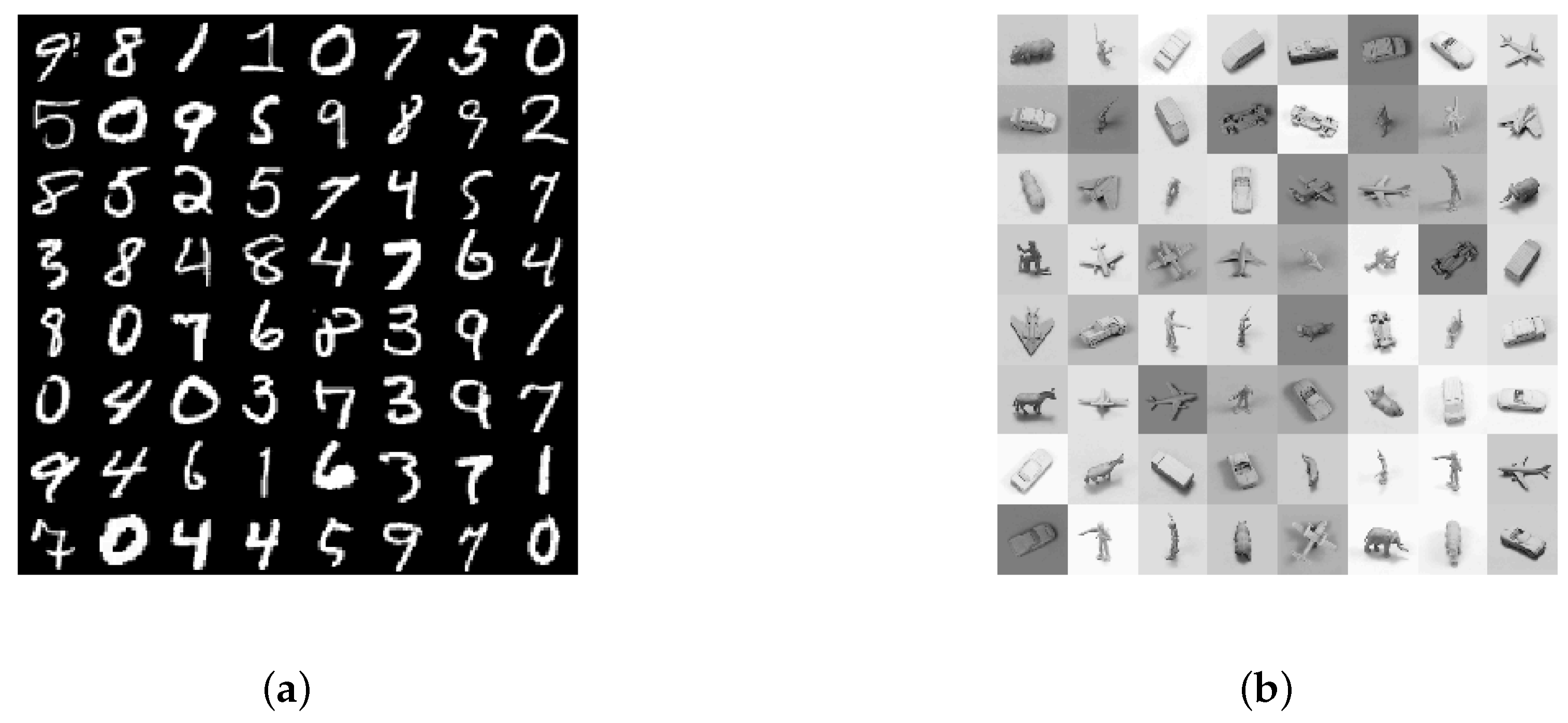
4.1.1. Datasets and Protocol

The left- and right-hand panels in Figure 3 show samples of the $MNIST$ and $NORB$ datasets, respectively. $MNIST$ is a benchmark computer vision dataset of images of ten handwritten digits (0 to 9), each image containing 28 × 28 gray-scale pixels [2]. The training and testing sets contained 60,000 and 10,000 images, respectively. The 10,000 images of the training set were retrained as the validation set. Pre-processing was carried out to divide each pixel by 255 to make it suitable for the RBM. For $NORB$, the benchmark 3D object recognition dataset, we selected a uniform-normalized set [3] containing 24,300 pairs of stereo images in the training set and 24,300 pairs of stereo images in the test set. The $NORB$ dataset included images in five generic categories: $cars$, $trucks$, $planes$, $animals$, and $humans$. Each image has 96 × 96 gray-scale pixel values, so each training example contains 2 × 96 × 96 = 18,432 dimensions. To reduce the computation, the outer part of the image was ignored and only the center 64 × 64 pixels was kept (since objects were mostly in the centers). Then, each image was resized to 48 × 48, yielding 2 × 48 × 48 = 4608 dimensions for each sample. Next, the procedure as suggested in [55] was implemented to train a Gaussian–Bernoulli RBM with a 4608–4000 architecture to convert the gray-scale images into binary variables. Finally, these 4000 variables were treated as the pre-processed data to evaluate the proposed algorithm.

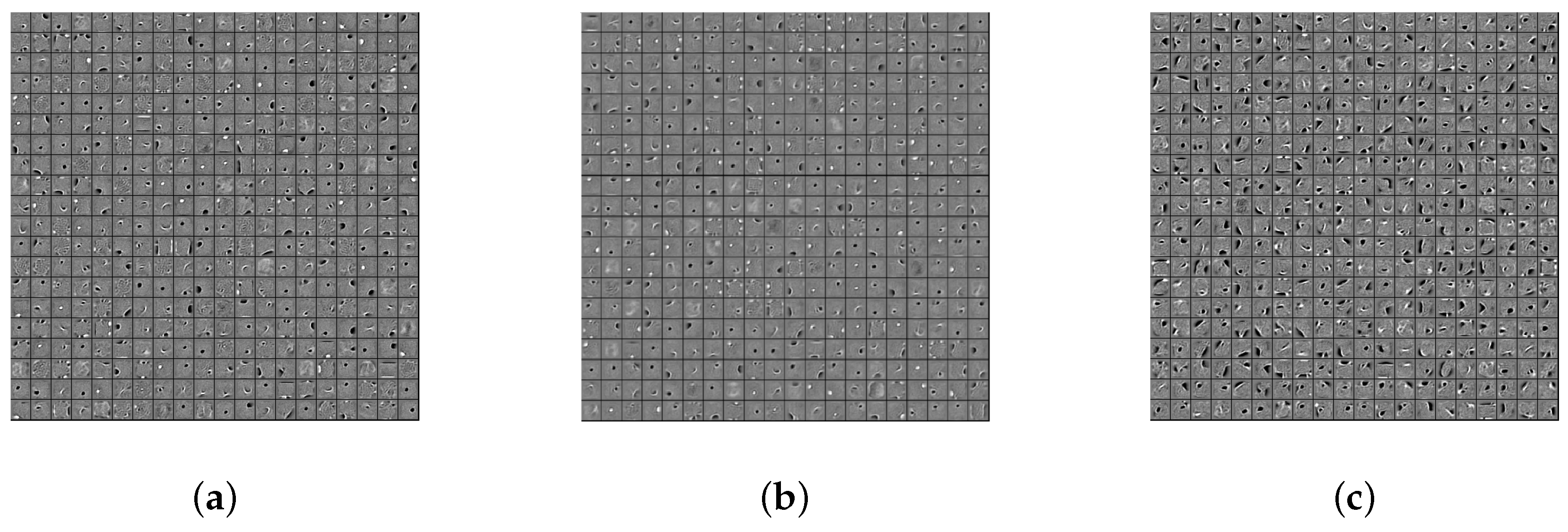
4.1.2. Feature Learning

In the first set of experiments, feature representations obtained by ML-RBM, ME-RBM, and CME-RBM are visualized. The $MNIST$ dataset along with the RBM with the 784–500 RBM architecture was used in this set of experiments. The left, middle, and right panels in Figure 4 illustrate feature detectors of RBMs trained with ML, ME, and CME criteria, respectively. The three panels demonstrate that the CME-trained RBM learned clearer edge detectors than the other two, most likely due to the sharper representations of the training images. Although a direct comparison of the three panels in Figure 4 does not explicitly reveal which provides better feature representations, the results confirm that the three RBMs indeed learned different feature representations. In Section 4.1.3, the object classifications are evaluated to compare the three learning criteria.

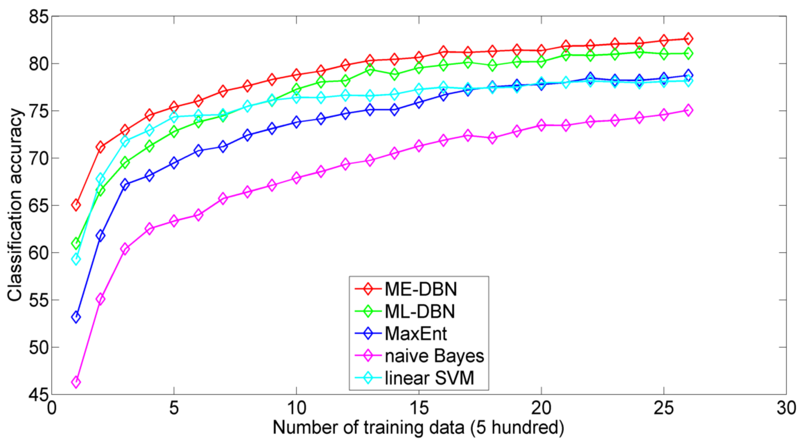
4.1.3. Classification Performance

The second set of experiments evaluates classification performance on the $MNIST$ and $NORB$ datasets. The DBNs were first estimated by ML, ME, and CME using training data without considering any label information. Next, another logistic layer was added on top of each model, and the combined model was treated as a DNN model. Then, the standard back-propagation training process was applied to the three models to refine their model parameters. The DNNs that are initialized by ML, ME, and CME, are still referred to as ML-DBN, ME-DBN, and CME-DBN throughout this paper. DBNs with 784–500–500–2000 and 4000–2000–2000 architecture were used for $MNIST$ and $NORB$, respectively.

Table 1. Classification error rates (in%) for DBNs with Maximum Likelihood (ML-DBN), Maximum Entropy (ME-DBN), and Constrained Maximum Entropy (CME-DBN) trained on 5%, 10%, 15%, and 20% of training data for the two object classification tasks: $MNIST$ and $NORB$.

Dataset	Method	5%	10%	15%	20%
MNIST	ML-DBN	4.90	3.39	2.75	2.45
	ME-DBN	4.84	3.30	2.57	2.31
	CME-DBN	4.66	3.11	2.46	2.17
NORB	ML-DBN	18.74	16.78	14.98	14.16
	ME-DBN	17.69	14.58	13.86	13.17
	CME-DBN	16.36	13.53	13.37	12.71

shows classification results for ML-DBN, ME-DBN, and CME-DBN under a limited amount of training data. To obtain the results in Table 1, we formed four new training sets by randomly selecting 5%, 10%, 15% and 20% amount of data from the original training set. These four training sets were used to estimate ML-DBN, ME-DBN, and CME-DBN and to conduct back-propagations to obtain three DNNs. Table 1 shows ME-DBN lowered the error rates compared to ML-DBN for small amounts of training data. The results also show that imposing constraints to the objective function (CME-DBN) improved the performance even further.

Table 2. Classification error rates (in%) for support vector machine (SVM), ML-DBN, ME-DBN, and CME-DBN using a full set of training data ($100\%$) for the two object classification tasks.

Dataset	SVM	ML-DBN	ME-DBN	CME-DBN
MNIST	1.40%	1.20%	1.04%	0.94%
NORB	11.60%	11.90%	10.80%	10.80%

evaluates the full set of training data ($100\%$), and compares classification error rates (in %) for support vector machine (SVM), ML-DBN, ME-DBN, and CME-DBN. For $MNIST$, ME-DBN gives a $1.04\%$ classification error rate, which already outperforms ML-DBN with $1.2\%$ [17], and SVM with $1.4\%$ [80]. Next, by using the weight decay and sparsity constraints, CME-DBN provided an even better $0.94\%$ classification error rate. For $NORB$, ME-DBN yielded a $10.80\%$ classification error rate, which already outperforms ML-DBN with $11.90\%$ [81], and SVM with $11.60\%$ [14]. On this database, CME-DBN provided similar improvements over ML-DBN and SVM. By progressively varying the amounts of available training data, the results of Table 1 and Table 2 confirms ME-DBN and CME-DBN outperforms ML-DBN by providing a better initial starting point for DNNs on these recognition tasks.

4.2. Experiments on Text Classification

In this set of experiments, we evaluate the proposed ME algorithm on three benchmark text classification tasks: $Newsgroup$, $Sector$, and $WebKB$. Similar to the object classification experiments in Section 4.1, α and β in Equation (18) are optimized empirically for CME. Also coinciding with Section 4.1, the three DBNs were first individually estimated by ML, ME, and CME, using the training data without any label information. For the three DBNs, the initial biases were set to zeros, and the weights were drawn from $\mathcal{N}(0,1)$.

4.2.1. Datasets and Protocol

The $Newsgroup$ dataset contains around 20,000 articles that are distributed evenly across 20 classes [82]. Of this set of documents, 13,000 and 5648 were selected for training and testing, respectively. For this task, stop-word removal and stemming were performed. A feature selection process was carried out to select the top 3000 words to generate the feature vector for each document.

The $Sector$ dataset contains more than 70 classes, which can be divided into a two-level hierarchy [83]. Only the 12 main categories in the top level with 9554 documents were used in the experiments. Finally, 6600 and 2867 documents were selected for training and testing, respectively. Stop-word removal was performed while stemming was not performed. The 3000 words with the highest mutual information were selected to generate the feature vector for each document.

The $WebKB$ dataset contains documents that were collected from web pages from the computer science departments of four universities [84]. The documents were divided into seven classes: $student$, $faculty$, $staff$, $project$, $course$, $department$, and $other$. In this study, the most popular four classes were selected: $student$, $faculty$, $project$, and $course$, which amounted to 4199 documents. From these documents, we selected 2900 and 1260 documents for training and testing, respectively. For this task, stop-word removal and stemming were not performed. A feature selection process was carried out on the entire word set by selecting the top 1000 words with the highest mutual information to form the feature vector for each document.

For the above three tasks, we followed the pre-processing steps (stemming, stoplist) as suggested in [69], where word count data were further scaled by dividing the total number of words in a document, subsequently allowing it to be interpreted as the probability for a word to appear in the document. Three DBN models were prepared to test performance, namely ML-DBN, ME-DBN, and CME-DBN. These three DBNs were first pretrained by ML, ME, and CME, respectively. Then, a logistic layer was added on the top of each model, and the standard back-propagation training was applied to refine the parameters. The training data were used for both initialization and back-propagation on these DNN models. The network architectures for $Newsgroup$, $Sector$, and $WebKB$ were 3000-1024-1024-20, 3000-2000-1500-12, and 1000-700-500-4, respectively. In addition to the three networks, several popular text classification algorithms are reported for comparison, including naive Bayes, SVM, and MaxEnt. For naive Bayes, a standard multinomial model with Laplace smoothing was used [85]. For SVM, a linear kernel support vector classifier was used [86]. For the maximum entropy classifier (MaxEnt), standard L2 penalized models were adopted [69]. Experiments for naive Bayes, SVM and MaxEnt were conducted using scikit-learn, a machine learning toolkit in Python [87] (Python Software Foundation, Beaverton, WA, USA).

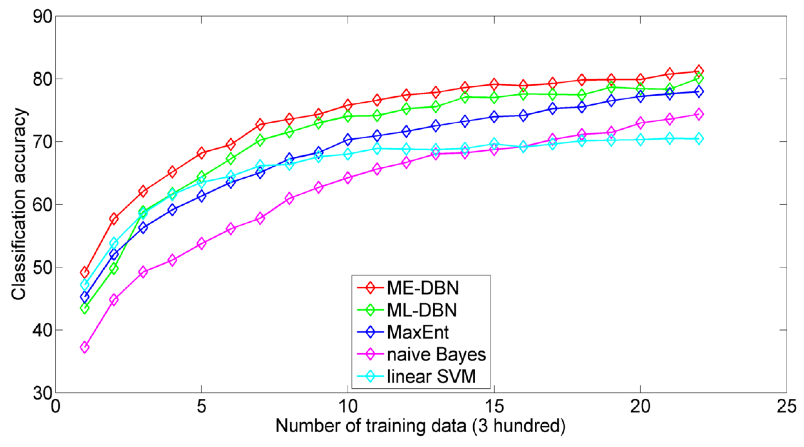
4.2.2. Classification Performance

We first compare ML-DBN and ME-DBN without weight decay and sparsity constraints (by setting $\alpha =0.0$ and $\beta =0.0$ in Equation (18)). Figure 5, Figure 6 and Figure 7 display the results of text classification with varying amounts of training data for $Newsgroup$, $Sector$, and $WebKB$, respectively. In each figure, the horizontal-axis and vertical-axis represent the amount of training data and classification accuracy rates, respectively.

The results in Figure 5 and Figure 6 show ME-DBN outperformed ML-DBN and all other approaches when training data was limited. Figure 7 shows ME-DBN outperforms MaxEnt, naive Bayes, and linear SVM, but only provided marginal improvements over ML-DBN. Since there are only four document classes in the $WebKB$ dataset of Figure 7, it is possible that over-fitting issues were less problematic compared to the $Newsgroup$ and $Sector$ tasks of Figure 5 and Figure 6. Overall, the results confirm that ME-DBN can offer improved performance over ML-DBN when the amount of training data is limited. Since the ME-DBN and ML-DBN algorithms differed only in their unsupervised pretraining process, the different classification capacities shown in Figure 5, Figure 6 and Figure 7 could only have resulted from the discovery of different local optima through the unique spaces of the different objective functions.

Table 3. Classification accuracies (in %) for ML-DBN, ME-DBN, and CME-DBN trained on 5%, 10%, 15%, and 20% of training data for the three text classification tasks: $Newsgroup$, $Sector$, and $WebKB$.

Dataset	Method	5%	10%	15%	20%
Newsgroup	ML-DBN	63.79	69.53	72.04	73.82
	ME-DBN	68.11	72.92	74.97	76.05
	CME-DBN	68.57	74.72	76.43	78.78
Sector	ML-DBN	46.64	58.85	63.05	67.29
	ME-DBN	53.44	62.09	66.69	69.54
	CME-DBN	53.57	62.37	66.64	70.06
WebKB	ML-DBN	81.22	87.61	89.28	90.95
	ME-DBN	82.76	88.17	89.20	90.95
	CME-DBN	84.00	89.28	90.47	91.98

shows classification results for ML-DBN, ME-DBN and CME-DBN under a limited amount of training data. The parameters α and β in Equation (18) were optimized empirically. Table 3 shows that CME-DBN outperforms ML-DBN consistently over the four different amounts of training data (5%, 10%, 15%, and 20%) for all of the $Newsgroup$, $Sector$, and $WebKB$ datasets.

Table 4. Classification accuracies (in%) for SVM, ML-DBN, ME-DBN, and CME-DBN using a full set of training data ($100\%$) for the three text classification tasks.

Dataset	SVM	ML-DBN	ME-DBN	CME-DBN
Newsgroup	75.07%	81.07%	82.62%	84.99%
Sector	74.36%	80.11%	81.23%	81.56%
WebKB	90.23%	92.45%	93.24%	93.57%

evaluates the full set of training data (100%), and compares classification accuracy rates (in %) for SVM, ML-DBN, ME-DBN and CME-DBN. By progressively varying the amounts of available training data, the results of Table 3 and Table 4 confirms ME-DBN and CME-DBN outperforms ML-DBN by providing a better initial starting point for DNNs. These finding were consistent with the recognition results in Table 1 and Table 2.

5. Conclusions

The present study demonstrates the effectiveness of ME learning for modeling DNN parameters using a DBN. Maximizing only the entropy offers robustness to over-fitting by keeping distributions as uniform and unbiased as possible. Object recognition results show ME-DBN consistently outperforms ML-DBN for different amounts of training data, and especially when training data is limited. In addition, we show the integration of weight decay and sparsity constraints (CME) enables even further improvements for ME learning. Text classification results similarly showed that DNNs initialized with ME-DBN and CME-DBN outperform those initialized by ML-DBN. Therefore, DBN training for a variety of tasks can benefit from ME learning and progressive regularization with the CME criteria.

References

1. Hopfield, J.J.; Tank, D.W. Computing with neural circuits—A model. Science 1986, 233, 625–633. [Google Scholar] [CrossRef] [PubMed]
2. LeCun, Y.; Bottou, L.; Bengio, Y.; Haffner, P. Gradient-based learning applied to document recognition. Proc. IEEE 1998, 86, 2278–2324. [Google Scholar] [CrossRef]
3. LeCun, Y.; Huang, F.J.; Bottou, L. Learning methods for generic object recognition with invariance to pose and lighting. In Proceedings of the 2004 IEEE Computer Society Conference on Computer Vision and Pattern Recognition, Washington, DC, USA, 27 June–2 July 2004; Volume 2, pp. 97–104.
4. Felleman, D.J.; van Essen, D.C. Distributed hierarchical processing in the primate cerebral cortex. Cereb. Cortex 1991, 1, 1–47. [Google Scholar] [CrossRef] [PubMed]
5. Lee, T.S.; Mumford, D.; Romero, R.; Lamme, V.A. The role of the primary visual cortex in higher level vision. Vis. Res. 1998, 38, 2429–2454. [Google Scholar] [CrossRef]
6. Rumelhart, D.E.; Hinton, G.E.; Williams, R.J. Learning representations by back-propagating errors. Nature 1988, 323, 533–536. [Google Scholar] [CrossRef]
7. Hinton, G.E. Connectionist learning procedures. Artif. Intell. 1989, 40, 185–234. [Google Scholar] [CrossRef]
8. Fu, L.; Hsu, H.H.; Principe, J.C. Incremental backpropagation learning networks. IEEE Trans. Neural Netw. 1996, 7, 757–761. [Google Scholar] [PubMed]
9. Lake, B.M.; Salakhutdinov, R.; Tenenbaum, J.B. Human-level concept learning through probabilistic program induction. Science 2015, 350, 1332–1338. [Google Scholar] [CrossRef] [PubMed]
10. Gopnik, A.; Glymour, C.; Sobel, D.M.; Schulz, L.E.; Kushnir, T.; Danks, D. A theory of causal learning in children: Causal maps and Bayes nets. Psychol. Rev. 2004, 111, 3–32. [Google Scholar] [CrossRef] [PubMed]
11. Mumford, D. On the computational architecture of the neocortex. Biol. Cybern. 1992, 66, 241–251. [Google Scholar] [CrossRef] [PubMed]
12. LeCun, Y.; Bengio, Y.; Hinton, G. Deep learning. Nature 2015, 521, 436–444. [Google Scholar] [CrossRef] [PubMed]
13. Smolensky, P. Information processing in dynamical systems: Foundations of harmony theory. In Parallel Distributed Processing; MIT Press: Cambridge, MA, USA, 1986; pp. 194–281. [Google Scholar]
14. Bengio, Y.; LeCun, Y. Scaling Learning Algorithms towards AI; MIT Press: Cambridge, MA, USA, 2007. [Google Scholar]
15. Ackley, D.H.; Hinton, G.E.; Sejnowski, T.J. A learning algorithm for Boltzmann machines. Cogn. Sci. 1985, 9, 147–169. [Google Scholar] [CrossRef]
16. Bengio, Y. Learning deep architectures for AI. Found. Trends Mach. Learn. 2009, 2, 1–127. [Google Scholar] [CrossRef]
17. Hinton, G.E.; Salakhutdinov, R.R. Reducing the dimensionality of data with neural networks. Science 2006, 313, 504–507. [Google Scholar] [CrossRef] [PubMed]
18. Hinton, G.E.; Osindero, S.; Teh, Y.W. A fast learning algorithm for deep belief nets. Neural Comput. 2006, 18, 1527–1554. [Google Scholar] [CrossRef] [PubMed]
19. Hinton, G.E. Training products of experts by minimizing contrastive divergence. Neural Comput. 2002, 14, 1771–1800. [Google Scholar] [CrossRef] [PubMed]
20. Deng, L. Three classes of deep learning architectures and their applications: A tutorial survey. APSIPA Trans. Signal Inf. Process. Available online: https://www.microsoft.com/en-us/research/publication/three-classes-of-deep-learning-architectures-and-their-applications-a-tutorial-survey/ (accessed on 7 July 2016).
21. Liu, F.; Liu, B.; Sun, C.; Liu, M.; Wang, X. Deep belief network-based approaches for link prediction in signed social networks. Entropy 2015, 17, 2140–2169. [Google Scholar] [CrossRef]
22. Ma, X.; Wang, X. Average Contrastive Divergence for Training Restricted Boltzmann Machines. Entropy 2016, 18, 35. [Google Scholar] [CrossRef]
23. Hinton, G.E. To recognize shapes, first learn to generate images. Prog. Brain Res. 2007, 165, 535–547. [Google Scholar] [PubMed]
24. Erhan, D.; Manzagol, P.A.; Bengio, Y.; Bengio, S.; Vincent, P. The difficulty of training deep architectures and the effect of unsupervised pre-training. In Proceedings of the 12th International Conference on Artificial Intelligence and Statistics (AISTATS), Clearwater Beach, FL, USA, 16–18 April 2009; pp. 153–160.
25. Larochelle, H.; Bengio, Y.; Louradour, J.; Lamblin, P. Exploring strategies for training deep neural networks. J. Mach. Learn. Res. 2009, 10, 1–40. [Google Scholar]
26. Bengio, Y.; Lamblin, P.; Popovici, D.; Larochelle, H. Greedy layer-wise training of deep networks. In Proceedings of the Neural Information Processing Systems (NIPS’06), Vancouver, BC, Canada, 3–8 December 2007; Volume 19, pp. 153–160.
27. Erhan, D.; Bengio, Y.; Courville, A.; Manzagol, P.A.; Vincent, P.; Bengio, S. Why does unsupervised pre-training help deep learning? J. Mach. Learn. Res. 2010, 11, 625–660. [Google Scholar]
28. Vincent, P.; Larochelle, H.; Lajoie, I.; Bengio, Y.; Manzagol, P.A. Stacked denoising autoencoders: Learning useful representations in a deep network with a local denoising criterion. J. Mach. Learn. Res. 2010, 11, 3371–3408. [Google Scholar]
29. Bengio, Y.; Simard, P.; Frasconi, P. Learning long-term dependencies with gradient descent is difficult. IEEE Trans. Neural Netw. 1994, 5, 157–166. [Google Scholar] [CrossRef] [PubMed]
30. Jaynes, E.T. Information theory and statistical mechanics. Phys. Rev. 1957, 106, 620–630. [Google Scholar] [CrossRef]
31. Schneidman, E.; Berry, M.J.; Segev, R.; Bialek, W. Weak pairwise correlations imply strongly correlated network states in a neural population. Nature 2006, 440, 1007–1012. [Google Scholar] [CrossRef] [PubMed]
32. Yeh, F.C.; Tang, A.; Hobbs, J.P.; Hottowy, P.; Dabrowski, W.; Sher, A.; Litke, A.; Beggs, J.M. Maximum entropy approaches to living neural networks. Entropy 2010, 12, 89–106. [Google Scholar] [CrossRef]
33. Haddad, W.M.; Hui, Q.; Bailey, J.M. Human brain networks: Spiking neuron models, multistability, synchronization, thermodynamics, maximum entropy production, and anesthetic cascade mechanisms. Entropy 2014, 16, 3939–4003. [Google Scholar] [CrossRef]
34. Nasser, H.; Cessac, B. Parameter estimation for spatio-temporal maximum entropy distributions: Application to neural spike trains. Entropy 2014, 16, 2244–2277. [Google Scholar] [CrossRef] [Green Version]
35. Ohiorhenuan, I.E.; Mechler, F.; Purpura, K.P.; Schmid, A.M.; Hu, Q.; Victor, J.D. Sparse coding and high-order correlations in fine-scale cortical networks. Nature 2010, 466, 617–621. [Google Scholar] [CrossRef] [PubMed]
36. Bell, A.J.; Sejnowski, T.J. An information-maximization approach to blind separation and blind deconvolution. Neural Comput. 1995, 7, 1129–1159. [Google Scholar] [CrossRef] [PubMed]
37. MacKay, D. Maximum entropy connections: Neural networks. In Maximum Entropy and Bayesian Methods; Springer: Dordrecht, The Netherlands, 1991; pp. 237–244. [Google Scholar]
38. Marrian, C.; Peckerar, M.; Mack, I.; Pati, Y. Electronic Neural Nets for Solving Ill-Posed Problems with an Entropy Regulariser. In Maximum Entropy and Bayesian Methods; Springer: Dordrecht, The Netherlands, 1989; pp. 371–376. [Google Scholar]
39. Szu, H.; Kopriva, I. Unsupervised learning with stochastic gradient. Neurocomputing 2005, 68, 130–160. [Google Scholar] [CrossRef]
40. Ingman, D.; Merlis, Y. Maximum entropy signal reconstruction with neural networks. IEEE Trans. Neural Netw. 1991, 3, 195–201. [Google Scholar] [CrossRef] [PubMed]
41. Choong, P.L.; Desilva, C.J.; Dawkins, H.J.; Sterrett, G.F. Entropy maximization networks: An application to breast cancer prognosis. IEEE Trans. Neural Netw. 1996, 7, 568–577. [Google Scholar] [CrossRef] [PubMed]
42. Bengio, Y.; Schwenk, H.; Senécal, J.S.; Morin, F.; Gauvain, J.L. Neural probabilistic language models. In Innovations in Machine Learning; Springer: Berlin, Germany, 2006; pp. 137–186. [Google Scholar]
43. Sarikaya, R.; Hinton, G.E.; Deoras, A. Application of deep belief networks for natural language understanding. IEEE/ACM Trans. Audio Speech Lang. Process. 2014, 22, 778–784. [Google Scholar] [CrossRef]
44. Yu, D.; Seltzer, M.L.; Li, J.; Huang, J.T.; Seide, F. Feature learning in deep neural networks-studies on speech recognition tasks. In Proceedings of the International Conference on Learning Representations, Scottsdale, AZ, USA, 2–4 May 2013; pp. 1–9.
45. Jing, H.; Tsao, Y. Sparse maximum entropy deep belief nets. In Proceedings of the 2013 International Joint Conference on Neural Networks (IJCNN), Dallas, TX, USA, 4–9 August 2013; pp. 1–6.
46. Wang, S.; Schuurmans, D.; Peng, F.; Zhao, Y. Boltzmann machine learning with the latent maximum entropy principle. In Proceedings of the Nineteenth Conference on Uncertainty in Artificial Intelligence, Edmonton, AB, Canada, 1–4 August 2002; Morgan Kaufmann Publishers Inc.: Burlington, MA, USA, 2002; pp. 567–574. [Google Scholar]
47. Mohamed, A.; Dahl, G.E.; Hinton, G. Acoustic modeling using deep belief networks. IEEE Trans. Audio Speech Lang. Process. 2012, 20, 14–22. [Google Scholar]
48. Hinton, G.E. A practical guide to training restricted boltzmann machines. In Neural Networks: Tricks of the Trade; Springer: Berlin, Germany, 2012; pp. 599–619. [Google Scholar]
49. Fisher, R.A. On an absolute criterion for fitting frequency curves. Messenger Math. 1912, 41, 155–160. [Google Scholar]
50. Chen, B.; Zhu, Y.; Hu, J.; Principe, J.C. System Parameter Identification: Information Criteria and Algorithms; Elsevier: Amsterdam, The Netherlands, 2013. [Google Scholar]
51. Chien, J.T.; Lu, T.W. Tikhonov regularization for deep neural network acoustic modeling. In Proceedings of the 2014 IEEE Spoken Language Technology Workshop (SLT), South Lake Tahoe, NV, USA, 7–10 December 2014; pp. 147–152.
52. Larochelle, H.; Bengio, Y. Classification using discriminative restricted Boltzmann machines. In Proceedings of the 25th International Conference on Machine Learning, Helsinki, Finland, 5–9 July 2008; pp. 536–543.
53. Lewicki, M.S.; Sejnowski, T.J. Learning nonlinear overcomplete representations for efficient coding. In Advances in Neural Information Processing Systems; MIT Press: Cambridge, MA, USA, 1998; pp. 556–562. [Google Scholar]
54. Tomczak, J.M. Application of classification restricted Boltzmann machine to medical domains. World Appl. Sci. J. 2014, 31, 69–75. [Google Scholar]
55. Salakhutdinov, R.; Hinton, G.E. Deep boltzmann machines. In Proceedings of the 12th International Confe-rence on Artificial Intelligence and Statistics (AISTATS), Clearwater Beach, FL, USA, 16–18 April 2009; Volume 5, pp. 448–455.
56. Wang, S.; Greiner, R.; Wang, S. Consistency and generalization bounds for maximum entropy density estimation. Entropy 2013, 15, 5439–5463. [Google Scholar] [CrossRef]
57. Pan, S.J.; Yang, Q. A Survey on Transfer Learning. IEEE Trans. Knowl. Data Eng. 2010, 22, 1345–1359. [Google Scholar] [CrossRef]
58. Lee, H.; Battle, A.; Raina, R.; Ng, A.Y. Efficient sparse coding algorithms. In Proceedings of the Neural Information Processing Systems (NIPS 2007), Vancouver, BC, Canada, 3–8 December 2007; Volume 20, pp. 801–808.
59. Raina, R.; Battle, A.; Lee, H.; Packer, B.; Ng, A. Self-taught learning: transfer learning from unlabeled data. In Proceedings of the 24th Annual International Conference on Machine Learning, Corvallis, OR, USA, 20–24 June 2007; pp. 759–766.
60. Tenenbaum, J.B.; Kemp, C.; Griffiths, T.L.; Goodman, N.D. How to grow a mind: Statistics, structure, and abstraction. Science 2011, 331, 1279–1285. [Google Scholar] [CrossRef] [PubMed]
61. Berger, A.L.; Pietra, V.J.D.; Pietra, S.A.D. A maximum entropy approach to natural language processing. Comput. Linguist. 1996, 22, 39–71. [Google Scholar]
62. Schneidman, E.; Still, S.; Berry, M.J.; Bialek, W. Network information and connected correlations. Phys. Rev. Lett. 2003, 91, 238701. [Google Scholar] [CrossRef] [PubMed]
63. Atick, J.J. Could information theory provide an ecological theory of sensory processing? Netw. Comput. Neural Syst. 1992, 3, 213–251. [Google Scholar] [CrossRef]
64. Lee, H.; Ekanadham, C.; Ng, A.Y. Sparse deep belief net model for visual area V2. In Proceedings of the Neural Information Processing Systems (NIPS), Vancouver, BC, Canada, 8–13 December 2008; pp. 873–880.
65. Sutskever, I.; Tieleman, T. On the convergence properties of Contrastive Divergence. In Proceedings of the Thirteenth Conference on Artificial Intelligence and Statistics, Sardinia, Italy, 13–15 May 2010; pp. 789–795.
66. Carreira-Perpinan, M.A.; Hinton, G.E. On Contrastive Divergence Learning. In Proceedings of the Tenth Workshop on Artificial Intelligence and Statistics, The Savannah Hotel, Barbados, 6–8 January 2005; pp. 59–66.
67. Toutanova, K.; Manning, C.D. Enriching the Knowledge Sources Used in a Maximum Entropy Part-of-Speech Tagger. In Proceedings of the 2000 Joint SIGDAT Conference on Empirical Methods in Natural Language Processing and Very Large Corpora, Morristown, NJ, USA, 1–8 October 2000; pp. 63–70.
68. Ratnaparkhi, A. A maximum entropy model for part-of-speech tagging. In Proceedings of the Conference on Empirical Methods in Natural Language Processing (EMNLP), Philadelphia, PA, USA, 17–18 May 1996; Volume 1, pp. 133–142.
69. Nigam, K. Using maximum entropy for text classification. In Proceedings of the IJCAI’99 Workshop on Machine Learning for Information Filtering, Stockholm, Sweden, 31 July–6 August 1999; pp. 61–67.
70. Wang, S.; Schuurmans, D.; Zhao, Y. The latent maximum entropy principle. ACM Trans. Knowl. Discov. Data 2012, 6, 8. [Google Scholar] [CrossRef]
71. Wang, S.; Schuurmans, D.; Zhao, Y. The Latent Maximum Entropy Principle. In Proceedings of the IEEE International Symposium on Information Theory, Lausanne, Switzerland, 30 June–5 July 2002; p. 131.
72. Berger, A. The Improved Iterative Scaling Algorithm: A Gentle Introduction. Carnegie Mellon University: Pittsburgh, PA, USA, Unpublished work. 1997. [Google Scholar]
73. Darroch, J.N.; Ratcliff, D. Generalized Iterative Scaling for Log-Linear Models. Ann. Math. Stat. 1972, 43, 1470–1480. [Google Scholar] [CrossRef]
74. Bilmes, J.A. A Gentle Tutorial on the EM Algorithm and Its Application to Parameter Estimation for Gaussian Mixture and Hidden Markov Models; Technical Rerport TR-97-021; International Computer Science Institute (ICSI): Berkeley, CA, USA, 1997. [Google Scholar]
75. Aharon, M.; Elad, M.; Bruckstein, A. K-SVD: Design of dictionaries for sparse representation. In Proceedings of the Signal Processing with Adaptative Sparse Structured Representations, Rennes, France, 16–18 November 2005; pp. 9–12.
76. Mairal, J.; Bach, F.; Ponce, J.; Sapiro, G. Online Dictionary Learning for Sparse Coding. In Proceedings of the 26th Annual International Conference on Machine Learning, Montreal, QC, Canada, 14–18 June 2009; pp. 689–696.
77. Gemmeke, J.F.; Virtanen, T.; Hurmalainen, A. Exemplar-Based Sparse Representations for Noise Robust Automatic Speech Recognition. IEEE Trans. Audio Speech Lang. Process. 2011, 19, 2067–2080. [Google Scholar] [CrossRef] [Green Version]
78. Kullback, S.; Leibler, R.A. On Information and Sufficiency. Ann. Math. Stat. 1951, 22, 79–86. [Google Scholar] [CrossRef]
79. Hinton, G.E.; Srivastava, N.; Krizhevsky, A.; Sutskever, I.; Salakhutdinov, R. Improving neural networks by preventing co-adaptation of feature detectors. 2012; arXiv:1207.0580. [Google Scholar]
80. Decoste, D.; Schölkopf, B. Training Invariant Support Vector Machines. Mach. Learn. 2002, 46, 161–190. [Google Scholar] [CrossRef]
81. Nair, V.; Hinton, G.E. 3-D object recognition with deep belief nets. In Proceedings of the 23rd Annual Conference on Neural Information Processing Systems, Vancouver, BC, Canada, 7–10 December 2009; pp. 1339–1347.
82. Joachims, T. A Probabilistic Analysis of the Rocchio Algorithm with TFIDF for Text Categorization. In Proceedings of the Proceedings of the Fourteenth International Conference on Machine Learning, Nashville, TN, USA, 2–12 July 1997; pp. 143–151.
83. McCallum, A.; Rosenfeld, R.; Mitchell, T.; Ng, A.Y. Improving Text Classification by Shrinkage in a Hierarchy of Classes. In Proceedings of the Fifteenth International Conference on Machine Learning, Madison, WI, USA, 24–27 July 1998; pp. 359–367.
84. Cardoso-Cachopo, A.; Oliveira, A.L.; Redol, R.A. An empirical comparison of text categorization methods. In International Symposium, String Processing and Information Retrieval; Springer: Berlin, Germany, 2003; pp. 183–196. [Google Scholar]
85. Zhai, C.; Lafferty, J. A study of smoothing methods for language models applied to information retrieval. ACM Trans. Inf. Syst. 2004, 22, 179–214. [Google Scholar] [CrossRef]
86. Fan, R.E.; Chang, K.W.; Hsieh, C.J.; Wang, X.R.; Lin, C.J. LIBLINEAR: A Library for Large Linear Classification. J. Mach. Learn. Res. 2008, 9, 1871–1874. [Google Scholar]
87. Pedregosa, F.; Varoquaux, G.; Gramfort, A.; Michel, V.; Thirion, B.; Grisel, O.; Blondel, M.; Prettenhofer, P.; Weiss, R.; Dubourg, V.; et al. Scikit-learn: Machine Learning in Python. J. Mach. Learn. Res. 2011, 12, 2825–2830. [Google Scholar]
Figure 1. Greedy layer-wise learning in a deep belief network (DBN).
Entropy 18 00251 g001
Figure 2. Hybrid model of the DBN after greedy layer-wise learning. The top two layers form the RBM and the bottom layers form a directed belief net.
Entropy 18 00251 g002
Figure 3. Samples from the (a) modified National Institute of Standards and Technology ( M N I S T ) and (b) NYU Object Recognition Benchmark ( N O R B ) databases.
Entropy 18 00251 g003
Figure 4. Features of 784–500 RBM trained with (a) Maximum Likelihood (ML-RBM); (b) Maximum Entropy (ME-RBM); (c) Constrained Maximum Entropy (CME-RBM).
Entropy 18 00251 g004
Figure 5. Classification accuracies with varying amounts of training sets on the N e w s g r o u p dataset.
Entropy 18 00251 g005
Figure 6. Classification accuracies with varying amounts of training sets on the S e c t o r dataset.
Entropy 18 00251 g006
Figure 7. Classification accuracies with varying amounts of training sets on the W e b K B dataset.
Entropy 18 00251 g007