Coupled Thermoelectric Devices: Theory and Experiment

Abstract

In this paper, we address theoretically and experimentally the optimization problem of the heat transfer occurring in two coupled thermoelectric devices. A simple experimental set up is used. The optimization parameters are the applied electric currents. When one thermoelectric is analysed, the temperature difference $\Delta T$ between the thermoelectric boundaries shows a parabolic profile with respect to the applied electric current. This behaviour agrees qualitatively with the corresponding experimental measurement. The global entropy generation shows a monotonous increase with the electric current. In the case of two coupled thermoelectric devices, elliptic isocontours for $\Delta T$ are obtained in applying an electric current through each of the thermoelectrics. The isocontours also fit well with measurements. Optimal figure of merit is found for a specific set of values of the applied electric currents. The entropy generation-thermal figure of merit relationship is studied. It is shown that, given a value of the thermal figure of merit, the device can be operated in a state of minimum entropy production.

1. Introduction

As the size of electronic devices decreases with further miniaturization techniques, there has been the problem of a large heat generation in small areas. Thermoelectric coolers are an alternative to efficiently dissipate heat generated in such conditions. The knowledge and control of irreversible phenomena that result in an increase of the temperature is, in this point of view, crucial. In many situations, the irreversibilities in the device are directly related to its optimum performance. Occasionally, optimal performance is obtained when the entropy generation is a low minimum under the operating constrictions. In this work, we study the thermal performance of a two-stage cooler with a dual purpose: (1) to theoretically model the transport of heat in the device and qualitatively compare theoretical predictions with experimental measurements of the temperature difference achieved between the hot and the cold faces in different operating conditions; and (2) to determine the relationship between global entropy production in the cooler and thermal performance measured by the thermal figure of merit [1]. The operating conditions are defined by the currents flowing in each of the stages of the cooler. The experimental device is similar to those reported in the literature [2,3,4,5,6,7], which are used for measuring thermal properties of thermoelectric materials or devices which are similar to the one studied here. Typically, the theoretical models used to describe transport phenomena in thermal devices are based on global energy balances at the ends and interfaces of the devices. Here, we use a local steady-state model that allows us to describe the spatial distribution of the relevant physical properties of the problem. Models similar to the one described here can be found in [3,4,8,9]. Our experimental results fit well with the theoretical predictions and the analysis on the relationship between entropy production and thermal performance reveals that, for each operating regime characterized by a specific thermal figure of merit, there are two entropy production regimes. The operating conditions of the device should be fitted in the lowest entropy production regime. This manuscript is divided in sections as follows: in Section 2, the two-stage cooler and the experimental procedure to measure the difference of temperature between the cold and the hot ends of the device are described as well as the operating conditions. In Section 3, a theoretical model used to study the heat transport and calculate the stationary temperature on the cold side, while the hot temperature remains constant, can be found. In Section 4, the thermoelectric parameters as well as the flowing electric currents in each of the stages are prescribed, and our theoretical results, comparison with measurements and results on the relation entropy production-thermal figure of merit are exposed and discussed. Finally, the concluding remarks are contained in Section 5.

2. Experimental Procedure

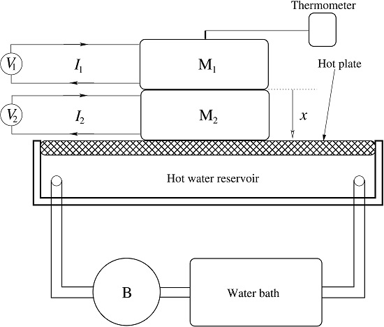
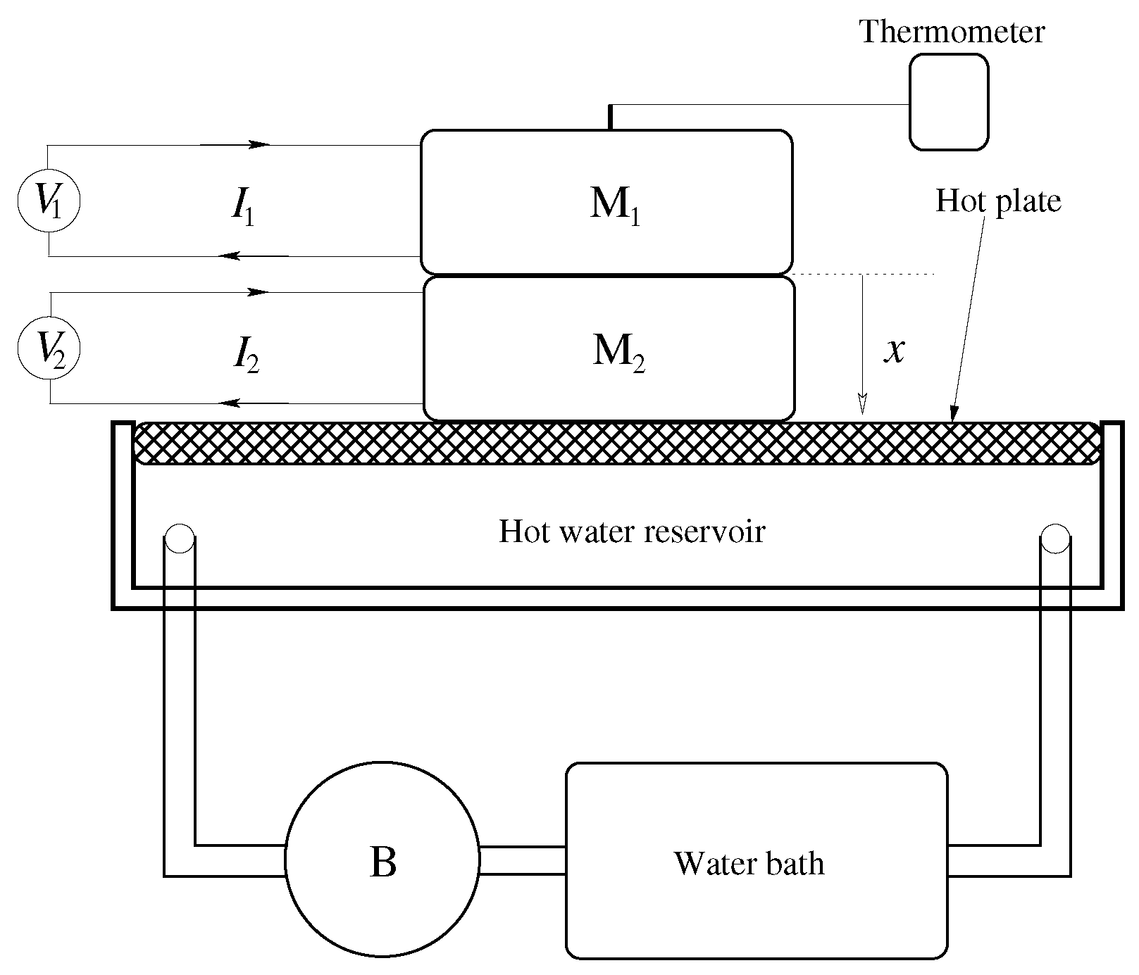
The experimental set-up consists of two Peltier modules connected thermally in series and electrically independent (see Figure 1). The thermoelectric modules are denoted by M. The modules are made of Bismuth Telluride alloys. The side length and width is $L=30$ mm and $h=3.6$ mm, respectively. The module array is mounted on a flat metal plate with measures 15 cm × 8 cm. This hot plate (or hot wall) is kept at a constant temperature by means of a warm bath. Hot water is continuously forced to circulate by a microprocessor dosing pump (Milton Roy, Houston, TX, USA) in a circuit containing a rectangular frame where the hot plate is located. The pump is denoted by B. Each direct electric current I is obtained from a regulated power supply V (Model 1696, B&K Precision Corporation, Yorba Linda, CA, USA) . The range of electric currents is between 0 to 1.517 A. In steady state, the temperature was measured in the geometrical center of the cold wall (top of module one $M_1$) by means of a thermocouple (K type) connected to a True RMS Multimeter (EX470, Extech Instruments, Nashua, NH, USA). The injected currents through the modules generate a heat flow from the cold to hot wall, thus the temperature in the cold wall is diminished. In order to avoid thermal decoupling, thermal paste (SILITEK Corporation, Taiwan) was placed between the two modules and the thermocouple-cold wall joint. The error in the temperature data was obtained by adjusting a normal distribution to the data at same points. The results of the experimental measurements are presented in Section 4.

3. Mathematical Model

The complete modelling of the experimental set-up can be very challenging. Instead, we can reduce the problem by considering the heat flux in a branch (n type) of the thin thermoelectric devices (see Figure 2). The devices are actioned by injecting an electric current I. The system is thus subjected to a Dirichlet boundary condition on the hot side $T_h$ of the thermoelectric device, and a Robin type one on the cold side $T_c$. Before focusing our attention to the mathematical model that describes the heat transfer in the coupled thermoelectric system, it is important to take into account the model that describes a single thermoelectric device, since it is the base for considering the coupled system.

3.1. Single Thermoelectric

The heat transport in a single thermoelectric thin film has been modelled previously in [1]. The temperature is described by a one-dimensional diffusion equation, considering the steady state and in dimensionless terms, it reads (see Appendix A in Reference [1])

$$0=\nu \frac{d^{2}T}{d{x}^2}+\beta J^2,$$

(1)

where the first term on the right-hand side denotes the diffusion and the second term is the Joule heating. Equation (1) is a particular case from the general heat-transport Equation (7) in [1]. Equation (1) is derived by observing in detail the effects of going to the micro and millimetric length scale where the stationary phenomena reported in this paper occur. In this way, the lengths of the involved experimental devices studied here yield a model that excludes memory, non-linear and non-local effects. The boundary conditions (also in dimensionless variables) can be written as:

$${\left.\frac{\partial T}{\partial x}\right]}_{x=-1}=\gamma JT(-1),T\left(1\right)=1.$$

(2)

The left boundary condition can be seen as a Robin-type since the temperature’s gradient is proportional to the temperature. The right (Dirichlet) boundary condition denotes the constant value of temperature on the hot side. The dimensionless coefficients in Equations (1) and (2) are defined as

$$\nu =\frac{K\tau }{\rho C_p{l}^2},\beta =\frac{J_0^2\tau }{\rho C_p\sigma T_h},\gamma =\frac{S_E{J}_{0}l}{K},$$

(3)

where $l=L/2$ is the half of the system’s length L, $\rho C_p$ is the volumetric heat capacity, $J_0$ is the magnitude of the electric density current through the thermoelectric, $T_h$ is the fixed temperature at the hot side, K is the thermal conductivity, σ is the electrical conductivity and $S_E$ is the Seebeck coefficient. The solution to Equation (1) reads

$$T\left(x\right)=a{x}^2+bx+c,$$

(4)

where the coefficients a, b and c are expressed as follows:

$$a=-\frac{\beta J^2}{2\nu },b=\frac{\gamma J+2a}{1+2\gamma J},c=1-a-b.$$

(5)

We must note that all of the coefficients in Equation (5) are functions of the applied electric density current J. The differences in temperature between the hot and cold sides are:

$$\Delta T_{single}=T\left(1\right)-T(-1)=2b.$$

(6)

On the other hand, the dimensionless entropy generation is given as [1]:

$$\dot{S}\left(x\right)=\frac{J^2}{T}+\frac{S_F}{S_J}\frac{1}{T^2}{\left(\frac{dT}{dx}\right)}^2,$$

(7)

where the coefficients are

$$S_J=\frac{J_0^2}{\sigma T_h},S_F=\frac{K}{l^2},$$

(8)

whereas the total entropy generation is calculated with the expression

$$\dot{\overline{S}}=\frac{1}{2}{\int }_{-1}^1\dot{S}\left(x\right)dx.$$

(9)

3.2. Coupled Thermoelectrics

Departing from the assumption that each of the thermoelectric devices behaves independently, as the single thermoelectric case (Equation (1)), and they only share a common boundary, the heat transport for the coupled system is modelled by a system of two one-dimensional differential equations, each for every thermoelectric device

$$0={\nu }_1\frac{d^2{T}_1}{d{x}^2}+{\beta }_1{J}_1^2,0={\nu }_2\frac{d^2{T}_2}{d{x}^2}+{\beta }_2{J}_2^2.$$

(10)

The subindex denotes the first (1) and second (2) device. In the same way as the single device case, the boundary conditions for the cold and hot sides are:

$${\left.\frac{\partial T_1}{\partial x}\right]}_{x=-1}=\gamma J_1{T}_1(-1),T_2\left(1\right)=1.$$

(11)

The coupling boundary conditions are

$${\gamma }_1{J}_1{T}_1\left(0\right)-{\left.\frac{d{T}_1}{dx}\right]}_{x=0}=\delta L\delta K{\gamma }_2{J}_2{T}_2\left(0\right)-\delta L\delta K{\left.\frac{d{T}_2}{dx}\right]}_{x=0},T_1\left(0\right)=T_2\left(0\right),$$

(12)

where the ratios between the lengths and the thermal conductivities are defined as $\delta L=L_1/L_2$ and $\delta K=K_2/K_1$, respectively. The coupling boundaries at $x=0$ are obtained from a heat balance and by equalling the temperatures of both devices. The solution to the system of Equation (10) reads:

$$T_1\left(x\right)=a_1{x}^2+b_{1}x+c_1,T_2\left(x\right)=a_2{x}^2+b_{2}x+c_2,$$

(13)

where the coefficients $a_i$, $b_i$ and $c_i$ are given as follows:

$$a_i=-\frac{{\beta }_i{J}_i^2}{2{\nu }_i},$$

(14)

$$c_1=\frac{\delta L\delta K(a_2-1)+\frac{a_1(2+{\gamma }_1{J}_1)}{1+{\gamma }_1{J}_1}}{\frac{{\left({\gamma }_1{J}_1\right)}^2}{1+{\gamma }_1{J}_1}-\delta L\delta K(1+{\gamma }_2{J}_2)}=c_2,$$

(15)

$$b_2=1-a_2-c_2,b_1=c_1({\gamma }_1{J}_1-\delta L\delta K{\gamma }_2{J}_2)+\delta L\delta K{b}_2.$$

(16)

It must be noted that the coefficients in Equation (5) all are functions of the injected electric density currents $J_i$. The differences in temperature between the hot and cold sides are

$$\Delta T_{coupled}=T_2\left(1\right)-T_1(-1)=a_2+b_2-a_1+b_1.$$

(17)

Finally, the total entropy generation is calculated with the expression

$$\dot{\overline{S}}=\frac{L_2}{L}\delta L\left({\int }_{-1}^0\dot{S_1}\left(x\right)dx+{\int }_0^1\dot{S_2}\left(x\right)dx\right),$$

(18)

where the total length of the system is $L=L_1+L_2$. The dimensionless entropy generation for each thermoelectric device $\dot{S_1}$ and $\dot{S_2}$ can be calculated in a similar manner as for a single device (see Equation (7)). The results obtained with the theoretical models for the single and the coupled thermoelectric systems are presented in the next section.

4. Results and Discussion

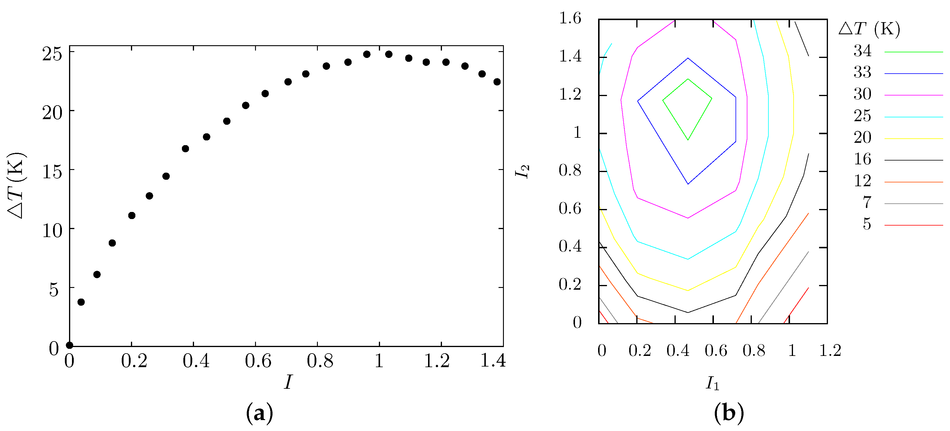
Before presenting and discussing the theoretical results, we depart from the experimental measurements for a single and a coupled system. Figure 3a shows the temperature difference between the hot and cold sides $\Delta T=T_h-T_c$ as a function of the injected electric current for a single thermoelectric device. In this figure, we can appreciate a parabolic behaviour with a maximum $\Delta T\approx$ 25 K, whereas Figure 3b presents elliptic isovalues of $\Delta T$ as function of the two electric currents, when the system is composed on two thermoelectric devices. For this array of devices, the maximum of temperature difference is $\Delta T\approx$ 34 K, that is, nine degrees of extra cooling are obtained when using two devices instead of a single one. For both cases, the single and two thermoelectric system, the electric current is normalized with $I_0=0.93$ A, which is the optimal current for a single device.

As in previous studies concerning thermoelectric devices [1,10,11], our theoretical results come from considering doped Silicon as working material, whose properties have been published before in [12]: $K=149$ Wm${}^{-1}$·K${}^{-1}$, $\sigma =35.5\times {10}^3$ ${\mathrm{\Omega }}^{-1}$·m${}^{-1}$, $S_E=440\times {10}^{-6}$ VK${}^{-1}$ and $a=88\times {10}^{-6}$ m${}^2$·s${}^{-1}$, where a is the thermal diffusivity; as the hot side temperature, we take $T_h=373.1$ K. We must note that these values do not correspond to our experimental case. However, since our model is a one-dimensional approximation of the heat transport, the objective is a qualitative comparison, and as it is shown in Figure 4, the aim is reached. 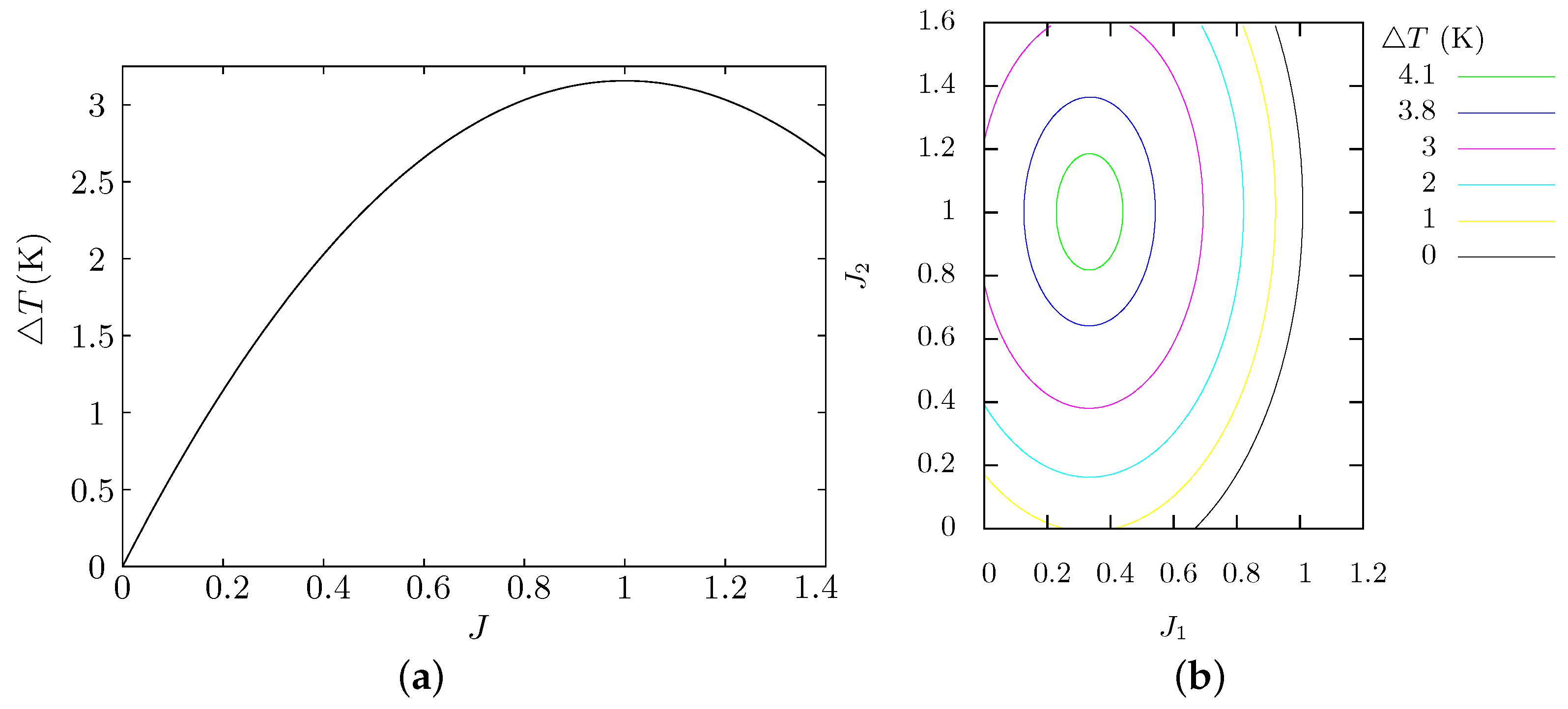Figure 4a shows the temperature difference $\Delta T=T_h-T_c$ as a function of the electric current for a single thermoelectric device (Equation (6)). Comparing with its experimental homologous, Figure 3a, the parabolic behaviour with a maximum is found. Figure 4b contains the dependence of $\Delta T$ when the system is composed on two thermoelectric devices (Equation (17)), presenting elliptic isovalues. Theoretical results (Figure 4) derived from a simple model agree qualitatively with the experimental ones (Figure 3) showing a maximum $\Delta T$ for a given set of electric currents. A quantitative comparison is far from been accomplished, since our model is a one-dimensional representation of a three-dimensional problem. However, if we calculate the percentage of the maximum extra cooling obtained when using two devices instead of a single one, that is $(\Delta T_{coupled}-\Delta T_{single})/\Delta T_{single}$, it is the same for both the experimental and theoretical results. The maximum extra cooling that could be reached is 36%.

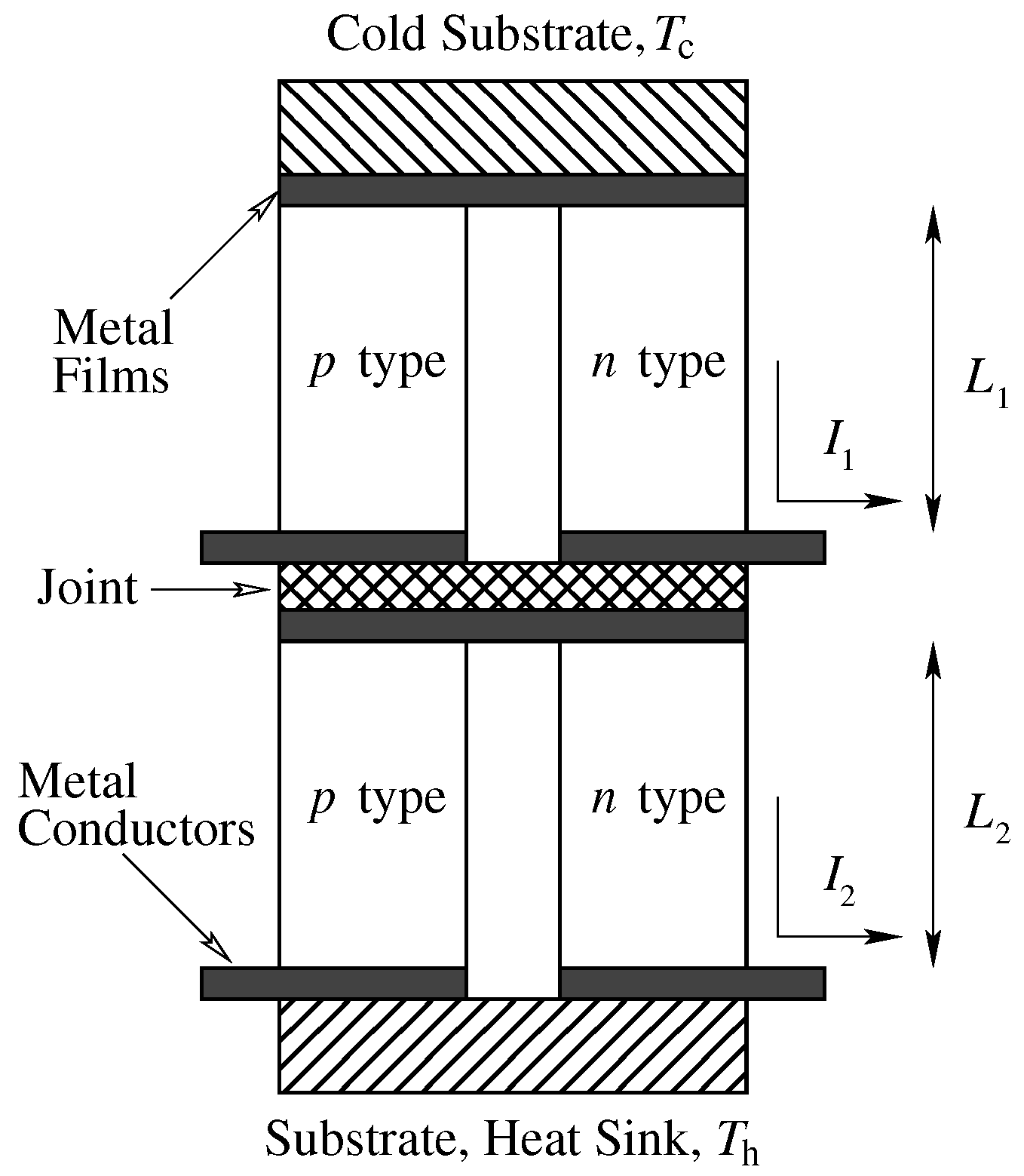
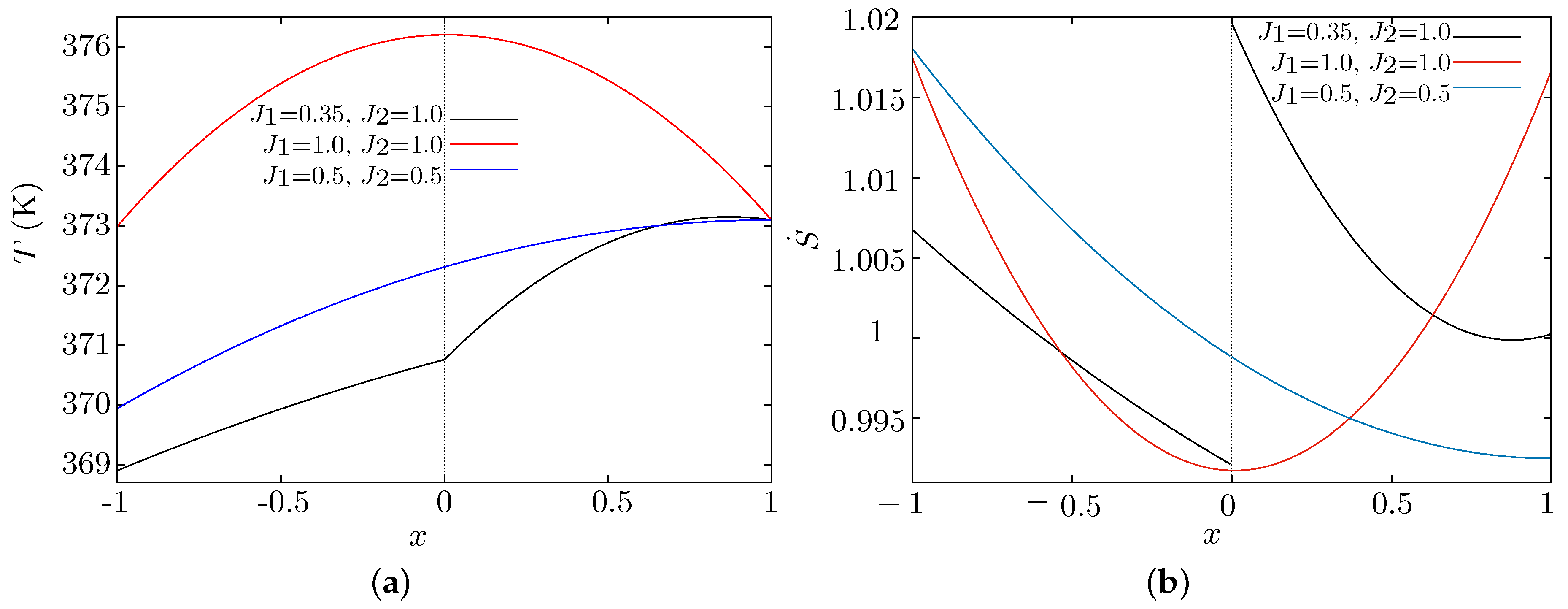
The temperature profiles along the x-axis for different sets of electric density currents are shown in Figure 5. The thermoelectric number one is contained in the domain (−1, 0), whereas the second one is in (0, 1). The cold ($T_c$) and hot ($T_h$) side temperatures are located at $x=-1$ and $x=1$, respectively. As seen in Equation (13), every segment of the profiles is a parabolic curve. The blue line has been previously obtained in the study of an optimal currents for a single thermoelectric [1]. In this case, the cooling obtained is 3.1 K. The black line denotes the profile for the optimal set of electric currents, obtaining a maximum cooling of 4.2 K, whereas the red line shows the case when the cooling is zero. For this case, the electric currents are high enough for the Joule effect dominate over the Peltier effect. In Figure 5b, it can be seen the theoretical profile of the local entropy production for different values of the electric current densities in the thermoelectric materials. As in Figure 5a, the black line represents the optimal case, the red one the zero cooling case, and the blue one another case with non-vanishing cooling. In the zero cooling, the entropy production is at the maximum at the cold and hot sides and is at a minimum at the coupling boundary. This minimum is explained by the fact that the temperature has a maximum and the temperature gradient vanishes at the same position. It is interesting that the minimum displaces toward the right ($x\approx 0.85$) when the current densities approach the optimal values. The discontinuity $x=0$ in the entropy production for the optimal case (black line) is due to the fact that the electric density current in each segment is distinct.

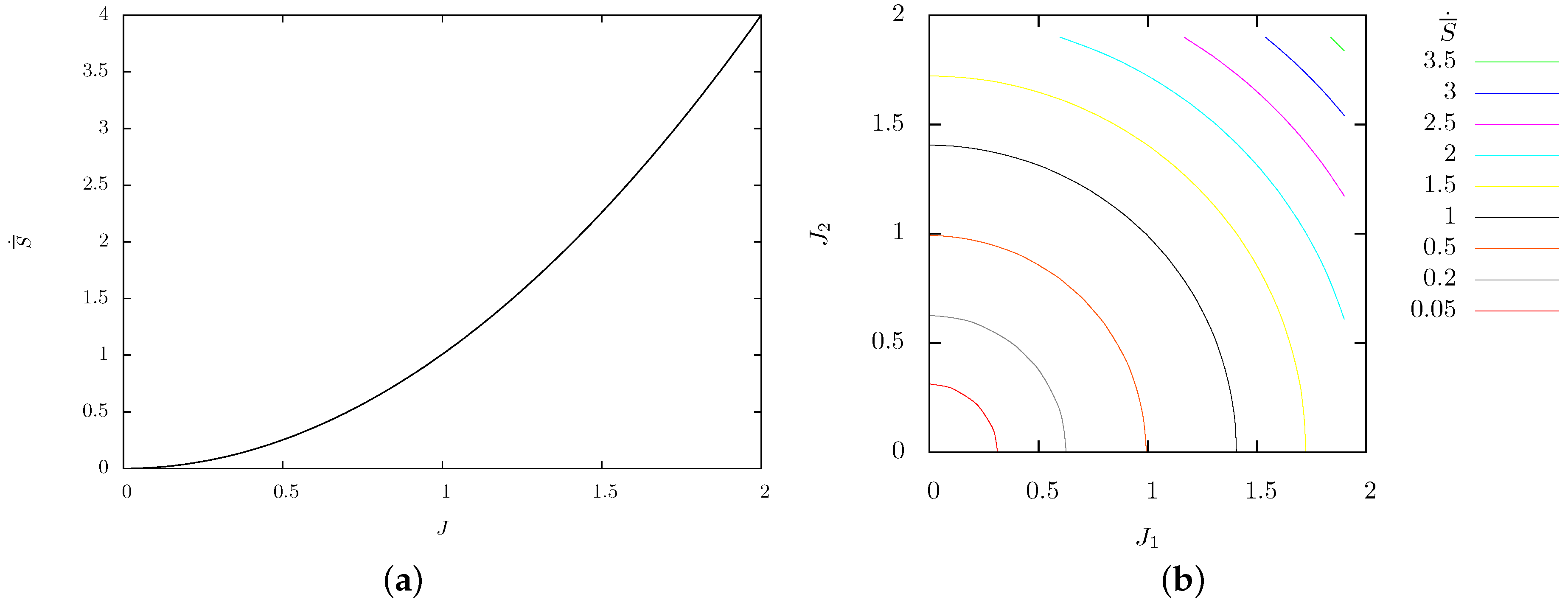
The total entropy generation $\dot{\overline{S}}$ in the devices can be seen in Figure 6. The dependence of the entropy for a single device shows a quadratic behaviour by increasing the electric current (see Figure 6a). For the two-device system, the entropy presents circular isolines increasing their magnitude as the electric currents are larger.

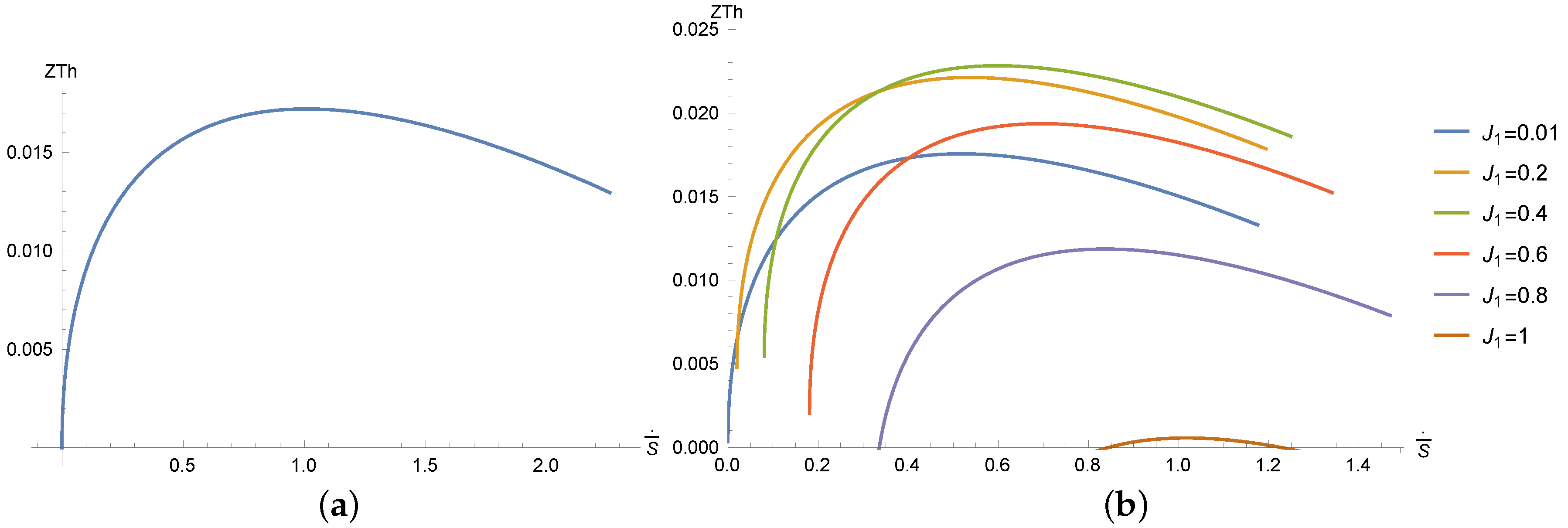
Finally, Figure 7 presents the thermal figure of merit $Z{T}_h=(2T_h\Delta T)/{(T_h-\Delta T)}^2$ as a function of the total entropy generation $\dot{\overline{S}}$. See the Appendix for a deduction of the thermal figure of merit $Z{T}_h$. We must note that both quantities depend on the electric density current applied to the system. For a single device (see Figure 7a), the figure of merit increases quickly as the total entropy generation does too, it reaches a maximum and then decreases slowly. We can note that aside from the maximum value, for each figure of merit value, there are two entropy production values. This is an interesting result since it provides evidence that the device can work in a smaller entropy production regime with the same thermal figure of merit. The same behaviour is found for the coupled devices (see Figure 7b). For $J_1=0.4$, the maximum of thermal figure of merit is larger than the maximum for a single device. This demonstrates the desirability of using two coupled thermoelectric materials rather than one. If $J_1$ is larger than 0.4, the maximum of the thermal figure of merit decreases drastically.

5. Conclusions

In this final section, we include some further comments that summarize our work. First, the heat transport in a set of coupled thermoelectric devices in a stationary state has been studied experimentally and theoretically. The temperature profiles show parabolic curves in each of the thermoelectric devices. The theoretical solutions compared with the experimental measurements concerning the temperature differences between the hot and the cold sides show a good qualitative agreement. An optimal cooling with respect to the injected electric currents has been found. The global entropy generation increases with the injected electric current. A maximum in the thermal figure of merit related with the global entropy production is found. It is worth mentioning the existence of two entropy production regimes for each value of the thermal figure of merit. This means that the device can be operated in a low entropy production state. An improvement of 36% in the performance of the coupled thermoelectric material with respect a single thermoelectric device is theoretically predicted. The results contained in this work may be useful to the design of coupled thermoelectric systems where the control of irreversible processes is an important issue.

References

1. Figueroa, A.; Vázquez, F. Optimal performance and entropy generation transition from micro to nanoscaled thermoelectric layers. Int. J. Heat Mass Transf. 2014, 71, 724–731. [Google Scholar] [CrossRef]
2. Yang, B.; Liu, J.L.; Wang, K.L.; Chen, G. Simultaneous measurements of Seebeck coefficient and thermal conductivity across superlattice. Appl. Phys. Lett. 2002, 80, 1758–1760. [Google Scholar] [CrossRef]
3. Bian, Z.; Zhang, Y.; Schmidt, H.; Shakouri, A. Thin film ZT characterization using transient Harman technique. In Proceedings of the 2005 International Conference on Thermoelectrics, Clemson, SC, USA, 18–24 June 2005; Volume 76.
4. Völklein, F.; Min, G.; Rowe, D.M. Modelling of a microelectromechanical thermoelectric cooler. Sens. Actuators 2006, 75, 95–101. [Google Scholar] [CrossRef]
5. Shin, W.; Ishikawa, M.; Nishibori, M.; Izu, N.; Itoh, T.; Matsubara, I. High-temperature thermoelectric measurement of B-doped SiGe and Si thin films. Mater. Trans. 2009, 50, 1596–1602. [Google Scholar] [CrossRef]
6. Ma, Y.; Ahlberg, E.; Sun, Y.; Iversen, B.B.; Palmqvist, A.E.C. Thermoelectric properties of thin films of bismuth telluride electrochemically deposited on stainless steel substrates. Electrochim. Acta 2011, 56, 4216–4223. [Google Scholar] [CrossRef]
7. Wojtas, N.; Grab, M.; Glatz, W.; Hierold, C. Stacked micro heat exchange system for optimized thermal coupling of microTEGs. J. Electr. Mater. 2013, 42, 2103–2109. [Google Scholar] [CrossRef]
8. Zhu, W.; Deng, Y.; Wang, Y.; Wang, A. Finite element analysis of miniature thermoelectric coolers with high cooling performance and short response time. Microelectr. J. 2013, 44, 860–868. [Google Scholar] [CrossRef]
9. Xuan, X.C.; Ng, K.C.; Yap, C.; Chua, H.T. A general model for studying effects of interface layers on thermoelectric devices performance. Int. J. Heat Mass Transf. 2002, 45, 5159–5170. [Google Scholar] [CrossRef]
10. Figueroa, A.; Vázquez, F. Spectral and finite difference solutions of the hyperbolic heat transport equation for thermoelectric thin films. Appl. Math. 2013, 4, 22–27. [Google Scholar] [CrossRef]
11. Rivera, I.; Figueroa, A.; Vázquez, F. Optimization of supercooling effect in nanoscaled thermoelectric layers. Commun. Appl. Ind. Math. 2016, 7, 98–110. [Google Scholar]
12. Zhou, Q.; Bian, Z.; Shakouri, A. Pulsed cooling of inhomogeneous thermoelectric materials. J. Phys. D Appl. Phys. 2007, 40, 4376–4381. [Google Scholar] [CrossRef]
13. Rowe, D.M. CRC Handbook of Thermoelectrics; CRC Press: Boca Raton, FL, USA, 1994. [Google Scholar]
Figure 1. Sketch of the experimental device, not drawn to scale. The coordinate system we use is shown. The thermoelectric modules are denoted by M i . The thermoelectric devices are actioned by imposing electric currents I i with DC voltage power supplies V i . The i denotes the first (1) and second (2) module. The rectangular plate is kept hot by circulating warm water in the reservoir. Temperature is measured in the top of module one ( M 1 ).
Entropy 18 00255 g001
Figure 2. Scheme of two coupled thermoelectric devices. This study is devoted to the thermal analysis of the thermoelectric materials denoted by n type. The devices are actioned by injecting an electric current I i . The thickness (width) is denoted by L i . The i denotes the first (1) and second (2) device.
Entropy 18 00255 g002
Figure 3. Δ T as function of the electric current. (a) single device; (b) coupled devices—experimental measurements.
Entropy 18 00255 g003
Figure 4. Δ T as function of the electric current. (a) single device; (b) coupled devices—theoretical predictions.
Entropy 18 00255 g004
Figure 5. (a) temperature distribution along coupled devices; (b) entropy generation profile. For clarity in the S ˙ profile comparison, the blue line is multiplied by a factor of 3.98 and the left part of the black line ( - 1 < x < 0 ) is multiplied by 7.99—theoretical predictions.
Entropy 18 00255 g005
Figure 6. Total entropy generation S ¯ ˙ as function of the applied electric current. (a) single device; (b) coupled devices—theoretical predictions.
Entropy 18 00255 g006
Figure 7. Thermal figure of merit Z T h as a function of the total entropy generation S ¯ ˙ . (a) single device; (b) coupled devices. In (b), each of the curves displayed is generated by varying J 2 from 0 to 1.6—theoretical predictions.
Entropy 18 00255 g007