Symmetric Fractional Diffusion and Entropy Production

Abstract

The discovery of the entropy production paradox (Hoffmann et al., 1998) raised basic questions about the nature of irreversibility in the regime between diffusion and waves. First studied in the form of spatial movements of moments of H functions, pseudo propagation is the pre-limit propagation-like movements of skewed probability density function (PDFs) in the domain between the wave and diffusion equations that goes over to classical partial differential equation propagation of characteristics in the wave limit. Many of the strange properties that occur in this extraordinary regime were thought to be connected in some manner to this form of proto-movement. This paper eliminates pseudo propagation by employing a similar evolution equation that imposes spatial unimodal symmetry on evolving PDFs. Contrary to initial expectations, familiar peculiarities emerge despite the imposed symmetry, but they have a distinct character.

1. Introduction

This paper follows a research program originating in the attempts of many authors to grapple with the physical phenomenon of anomalous diffusion [1,2,3,4] using extraordinary differential equations, which employ fractional calculus [5]. Fractional evolution equations use local and non-local [6,7] fractional derivatives defined in a variety of ways leading to interesting features in their solutions, for recent examples see [6,7,8,9]. Such fractional evolution equations have also developed into other applications (e.g., [10]) and modern techniques for computing the values of their solution functions have advanced [11,12,13,14]. In [15] we introduced the idea that the superdiffusion regime arising from an equation proposed for anomalous diffusion,

$$\frac{{\partial }^{\gamma }}{\partial t^{\gamma }}P(x,t)=\frac{{\partial }^2}{\partial x^2}P(x,t),$$

(1)

for $1\le \gamma \le 2$ and P being a probability density function (PDF), had implications beyond anomalous diffusion [5,16,17,18]:

Diffusion and wave propagation are often conceived as representatives of different and distinct worlds, both mathematically and physically. But the regime that (1) represents is not merely anomalous in terms of diffusion. Its existence, in which a single parameter, γ, smoothly transforms between the iconic diffusion and wave equations, opened a way to build a continuous bridge between the distinct worlds [15].

Physically, it is a bridge between irreversible and reversible processes: dissipative evolution smoothly maps into deterministic dynamics. Mathematically, partial differential equation (PDE) characteristics, responsible for propagation, emerge from an equation with none. This remarkable regime is not the only one. A fundamentally different equation family compared to (1) is

$$\frac{\partial }{\partial t}P(x,t)=\frac{{\partial }^{\alpha }}{\partial x^{\alpha }}P(x,t),$$

(2)

for $1\le \alpha \le 2$, which is fractional in space rather than time, and which also bridges between the diffusion equation and the half-wave equation, raising similar issues [17,18,19,20,21].

There are several essential differences between these two bridging families. We have explored the semi-infinite domain in (1), while (2) is on an infinite one. The fractional derivative in (1) can be thought of as being rooted in the Laplace transform, while that of (2) is Fourier based. The probability density functions (PDFs) of (1) are H-functions with all moments known [5,15,16], while those of (2) are Lévy stable densities with heavy tails and divergent moments (e.g., [17,19]).

However, in terms of the broader issues the similarities are more striking. Both one-parameter families of probability densities produce well-defined entropy and entropy production rates within the domain [5,15,16,17,18,19,20,21]. These PDFs share scaling properties inherited from their differential equations. The resulting entropy production rates have an unexpected property: as one moves away from the diffusion limit they increase [5,15,16,17,18,19]! We named this the entropy production paradox [15,22]. In both cases entropy can be found to have a maximum in between the bridging regime after a given time, making entropy unsuitable as a means to order processes in terms of relative irreversibility. While we have endeavored to rehabilitate entropy in an ordering role [5,15,16,17,18,19], the results have not been as robust as those from employing the Kullback–Leibler entropy [20,21]. Moreover, these extraordinary properties are insensitive to generalizations of the definition of entropy: they persist for Tsallis and Renyi Entropies too [16,18,19].

In our work, PDFs approach propagating delta functions in the wave limit for both cases. Before that limit, the moving peaks of skewed density functions are what map into the delta functions in the wave limit. They have moving peaks that sink while they broaden. In the wave limit they go over to moving delta functions. The pre-limit movement, which we call pseudo propagation, was first studied [15] in terms of the spatial movements of moments of H-function PDFs. Subsequently when dealing with the evolution of stable distributions alternative approaches to movement were necessary in the absence of moments [17,18,19]. Such movement was at the heart of our approach to avoid the maxima in the entropy emerging over the bridging regime. Some of these results have been recently reproduced [23].

Asymmetry is fundamental for the pseudo propagation in both cases. In (1) we used an asymmetric semi-infinity domain. In the other case, the PDFs are inherently skewed reflecting the inherent asymmetry of the half-wave equation occurring in the wave limit. In this paper we aim to control for pseudo propagation by exploring what happens when it is eliminated. To accomplish this we consider an extraordinary differential equation that has similar properties to those in the pseudo propagation cases, but without the spatial asymmetry. This implies a space fractional diffusion equation. The classical diffusion equation,

$$\frac{\partial }{\partial t}P(x,t)=D\frac{{\partial }^2}{\partial x^2}P(x,t),$$

(3)

clearly fits into this class. In the following we extend the symmetry of the diffusion equation into fractional evolution equations in an intuitive and precedented manner, although more complex symmetry preserving options are possible [24].

We find that even in the absence of pseudo propagation many of the properties of previous regimes persist, as do the excellent ordering features of the Kullback–Leibler entropy. Moreover the entropy production rate still increases as one moves away from the diffusion limit. However, the other end of the bridging regime is no longer the wave equation or even an evolution equation, so this cannot be regarded as paradoxical as such, but it demonstrates that pseudo propagation is not required for these phenomena.

A maximum for entropy does occur in the computed regime, but, unlike the asymmetric cases, it is difficult to find and it appears to occur within a narrow interval of time.

2. Space Symmetric Extraordinary Differential Equation

To achieve evolving symmetric PDFs we extend the spatial symmetry of the classical diffusion equation. This suggests the need for a symmetric fractional derivative, which has the same value in the forward and reverse directions. In conventional first derivatives they are not the same because differentials have an inherent directionality. Generalizations of derivatives must reflect this. One option that captures such symmetry is a weighted sum [25] given as,

$$\frac{d^{\alpha }}{{d\left|x\right|}^{\alpha }}=-\frac{1}{2cos(\pi \alpha /2)}\left[\frac{d^{\alpha }}{d{x}^{\alpha }}+\frac{d^{\alpha }}{d{(-x)}^{\alpha }}\right];\alpha \ne 1.$$

(4)

The cosine is a consequence of the Fourier definition of the fractional derivatives, which requires the consideration of ${(\pm ik)}^{\alpha }$. A branch cut is made to exclude singular cases. $\alpha =1$ is a special case because both the cosine and the sum of derivatives vanish. In terms of the Fourier transform, $\mathcal{F}\{P\}={\int }_{-\infty }^{\infty }P(x)e^{+ikx}\mathrm{d}x$, this becomes simply,

$$\frac{{\partial }^{\alpha }}{{\partial \left|x\right|}^{\alpha }}P(x)={\mathcal{F}}^{-1}{\{-|k|}^{\alpha }\mathcal{F}\{P(x)\}\}.$$

(5)

Note the choice of sign in the argument of $\mathcal{F}$’s exponential for its definition. This convenient choice makes $\mathcal{F}$ produce the characteristic function of a PDF.

When $\alpha =2$ this derivative agrees with the normal second derivative. However, when $\alpha =0$ the inconsistent outcome for the zeroth derivative,

$$P(x)\ne {\mathcal{F}}^{-1}\{-\mathcal{F}\{P(x)\}\},$$

(6)

makes the $\alpha =0$ case unacceptable. Thus, $0<\alpha \le 2$. This difficulty with the inconsistency of the $\alpha =0$ case anticipates computational challenges near 0, which are discussed below.

If we think in terms of an evolution equation for a PDF and equate the derivative in (5) to the time derivative of $P(x,t)$ we find

$$\frac{\partial }{\partial t}P(x,t)=\frac{{\partial }^{\alpha }}{{\partial \left|x\right|}^{\alpha }}P(x,t),$$

(7)

which captures (3) for $\alpha =2$ and imposes spatial symmetry for acceptable α, while retaining the scaling properties of the asymmetric cases described above.

The Fourier transform of the density function $P(x,t)$ from (7) with initial condition $P_{\alpha }(x,0)=\delta (x)$ is $\widetilde{P_{\alpha }}(k,t)$, with

$$\widetilde{P_{\alpha }}(k,t)={exp(-|k|}^{\alpha }t).$$

(8)

This is the characteristic function of a stable distribution without skewness and vanishing mean, valid for $0<\alpha \le 2$. In particular

$$\widetilde{P_{\alpha }}(k,t)=\mathcal{F}\left\{\mathbf{S}\left(\left.x\right|\alpha ,0,t^{1/\alpha },0;0\right)\right\}.$$

(9)

where the stable distribution, $\mathbf{S}\left(\left.x\right|\alpha ,\beta ,\gamma ,\delta ;n\right)$ (where this γ is not to be confused with the γ used above), generally has an infinite domain. In this case, $\alpha \in (0,2]$, $\beta =0$, $\gamma =t^{\frac{1}{\alpha }}$, $\delta =0$, and $n=0$ for details see [26].

Stable distributions have been used to characterize Lévy flight diffusive processes [25,27,28,29]. Such processes have been represented in the literature by (7) [25] and used to describe Lévy flights modeled by a Poisson waiting time with a Lévy distribution for the jump lengths [27,28,29]. Furthermore, the observed power law time behavior of the width of a stable distribution and—more generally—also of the solutions of time-fractional diffusion equations has interesting connections to relaxation processes in hierarchical structures [30,31] which are of importance in turbulent diffusion but also in glassy relaxation processes [30,32]. This is especially so for relaxation processes close to the glass transition power law and stretched exponential models, which provide viable alternatives in modeling different types of processes captured in the size of the exponents. However, our goal is not to connect stable distributions to random walks or relaxation processes in complex systems, but to examine how entropies and entropy production vary in the absence of pseudo propagation.

3. Symmetric Solutions and Entropy

From (9) we find

$$P_{\alpha }(x,t)=\mathbf{S}\left(\left.x\right|\alpha ,0,t^{1/\alpha },0;0\right)=\frac{1}{t^{1/\alpha }}\mathbf{S}\left(\left.\frac{x}{t^{1/\alpha }}\right|\alpha ,0,1,0;0\right),$$

(10)

where the scaling property of stable distributions was used. By design, $P_{\alpha }$ is symmetric, unimodal, and centered at $x=0$ [19,26].

The asymptotic behaviors of the tails for $0<\alpha \le 2$ are known [26]

$$\begin{array}{cc}\hfill P_{\alpha }(x,t)=\mathbf{S}\left(\left.x\right|\alpha ,0,t^{1/\alpha },0;0\right)& \sim \alpha t{c}_{\alpha }{\left|x\right|}^{-(\alpha +1)}(x\to \pm \infty ),\hfill \end{array}$$

(11)

with $c_{\alpha }=sin(\frac{\alpha \pi }{2})\Gamma (\alpha )/\pi$ and $\Gamma (\alpha )$ being the Gamma function.

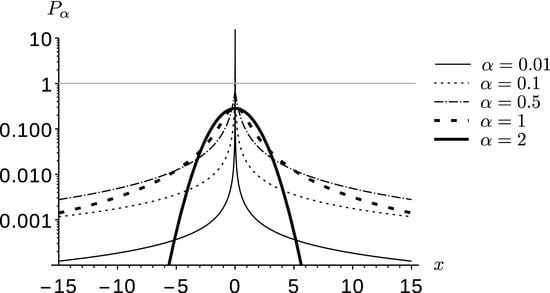
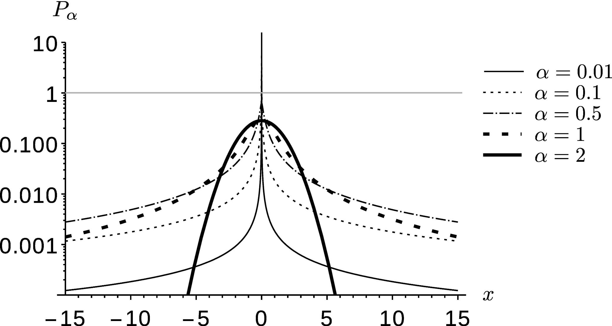
In Figure 1 the logarithm of the familiar distributions such as the Cauchy ($\alpha =1$) and the Gaussian distribution ($\alpha =2$) are plotted with other distributions to gain a sense of how the densities change with α. It is clear that all of these graphs are symmetric about $x=0$, as intended. For $\alpha =2$ (Gaussian) the graph is a simple parabola. As α decreases the tails rise and the central peak rapidly grows and strongly sharpens. As α approaches zero, the central peak grows larger than 1, which proves to be qualitatively significant when considered in terms of entropy.

The scaling behavior (10) makes the new variable

$$\eta =\frac{x}{t^{1/\alpha }},$$

(12)

useful, leading to the following definition,

$$G_{\alpha }^{}(\eta )=\mathbf{S}\left(\left.\eta \right|\alpha ,0,1,0;0\right).$$

(13)

It follows that

$$P_{\alpha }(x,t)=\frac{1}{t^{1/\alpha }}{G}_{\alpha }\left(\frac{x}{t^{1/\alpha }}\right),$$

(14)

which is normalized independent of time,

$${\int }_{-\infty }^{\infty }{P}_{\alpha }(x,t)\mathrm{d}x={\int }_{-\infty }^{\infty }{G}_{\alpha }(\eta )\mathrm{d}\eta =1.$$

(15)

Thus, the Shannon entropy is

$$\begin{array}{cc}\hfill S_{\alpha }(t)& =-{\int }_{-\infty }^{\infty }P(x,t)lnP(x,t)\mathrm{d}x=\frac{1}{\alpha }lnt-{\int }_{-\infty }^{\infty }{G}_{\alpha }^{}(\eta )ln{G}_{\alpha }^{}(\eta )\mathrm{d}\eta .\hfill \end{array}$$

(16)

Note that $S_{\alpha }(1)$ is just minus the time-independent integral.

A similar approach was also utilized by Haubold & Mathai [33,34] to analyze experimental solar neutrino data sets in order to investigate the underlying processes and the scaling of its PDFs.

4. Entropy Properties of the Symmetric Regime

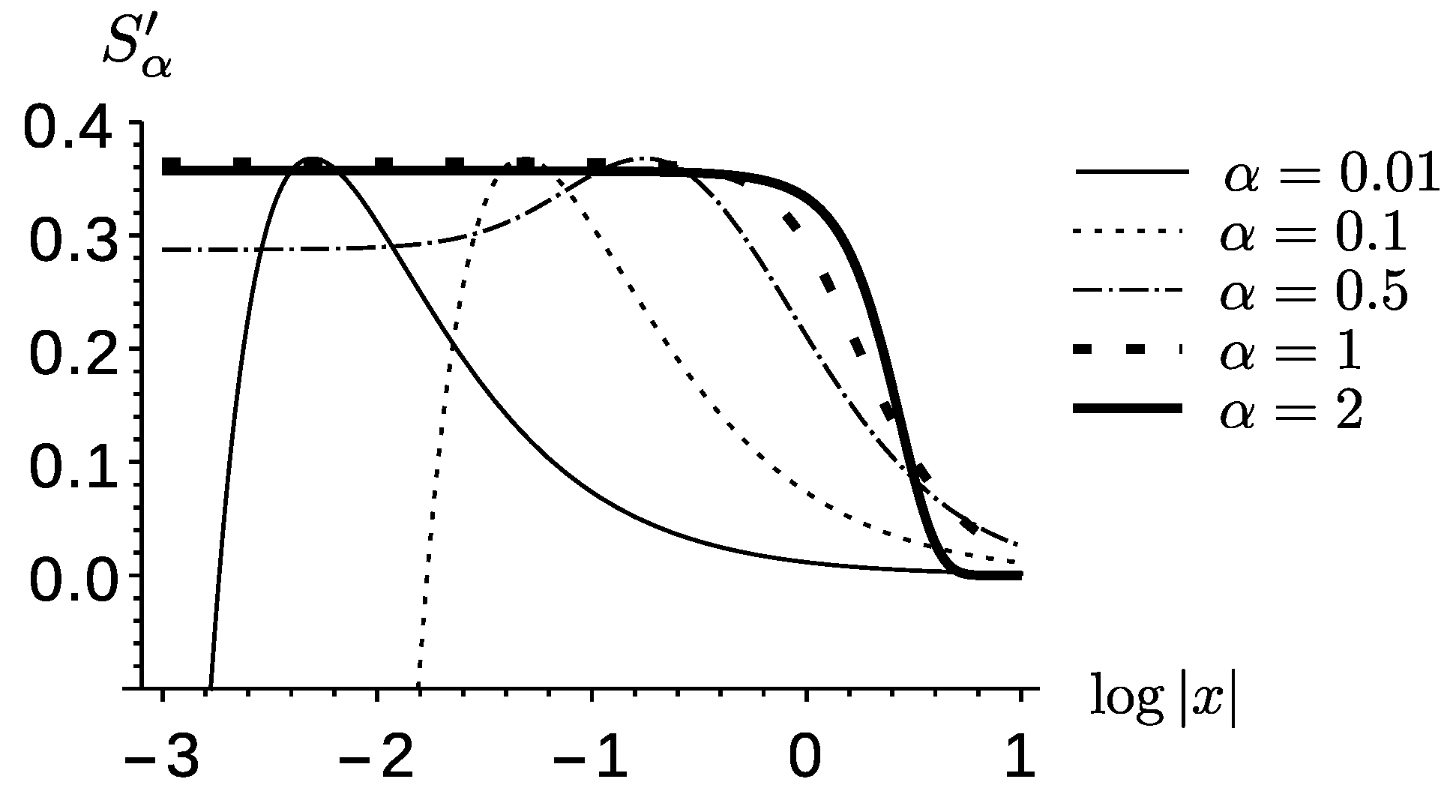
The Shannon kernel, $S_{\alpha }^{\prime }(x,t)=-P_{\alpha }(x,t)ln{P}_{\alpha }(x,t)$, is plotted for $t=1$ against x for several values of the parameter α in Figure 2. It shows the consequence of the tall sharp core of the PDF at low enough α. For values of the PDF above 1 the logarithm changes sign leading to a narrow negative core and twin maxima in the kernel. This effect increases with decreasing α, as a consequence of the increasing value of $P_{\alpha }(x,1)$ with decreasing α.

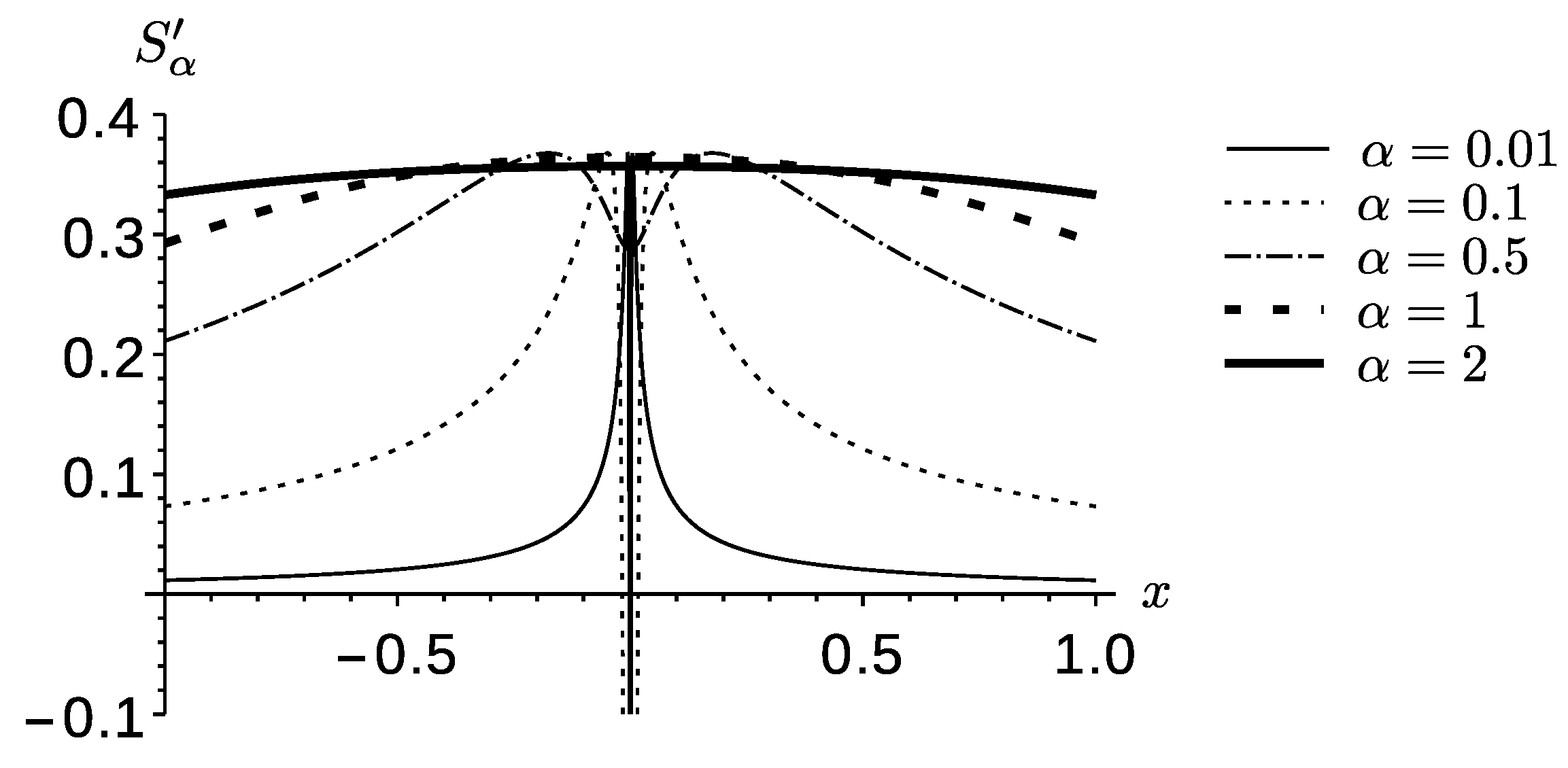
Figure 3 tells us more about how the negative core changes with α. The negative core of Figure 2 appears on the left side of the plot. While α’s above 1 are relatively constant toward the left, all of the cases with lower α exhibit maxima and strongly decrease toward the left. The lowest values of α represent functions that decrease most rapidly.

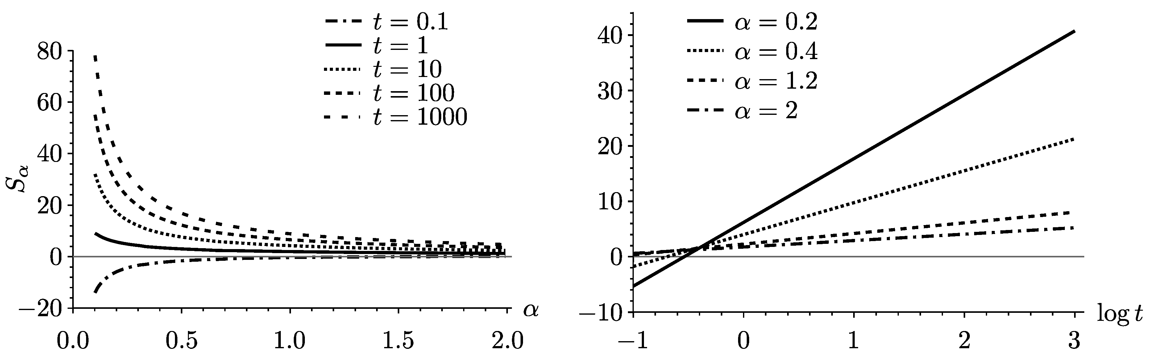
Figure 4 depicts the entropy $S_{\alpha }(t)$ in two ways. It is shown on the left as a function of α for different values of t, and on the right as a function of $logt$ for different values of α.

It increases monotonically with decreasing α for large t and decreases monotonically for short times. The derivative of $S_{\alpha }(t)$ with respect to α can only vanish,

$$\begin{array}{cc}\hfill \frac{\text{d}S}{\text{d}\alpha }& =-\frac{1}{{\alpha }^2}lnt+\frac{\text{d}{S}_{\alpha }(1)}{\text{d}\alpha }=0,\hfill \end{array}$$

(17)

for $t<1$, as the left side of Figure 4 indicates that the second term in (17) is always negative. It is worth noting that as α approaches 0, computation becomes more problematic. For the purposes of this paper we generally did not present results less than $\alpha \sim 0.1$ for this reason. Exploring very small values of α is a matter of ongoing investigation, but meanwhile discussion is limited to the domain actually computed. In the case of the second term in (17), it is an open question whether unknown sign changes exist for very small values of α.

If it vanishes at some critical $t=t_c$, for some α, then

$$\begin{array}{c}\hfill ln{t}_c=-{\alpha }^2\left|\frac{\text{d}{S}_{\alpha }(1)}{\text{d}\alpha }\right|.\end{array}$$

(18)

The second factor is decreasing in magnitude with α based on Figure 4. Any maximum of $S_{\alpha }$ in the computed interval must occur between the small-time increasing behavior and the large-time decreasing one. That means the $t_c$ should occur earlier for large α than for small α, so that increasing for small α and decreasing for large α coexist. Based on the plot the time interval where this can occur is $0.1<t<1$. 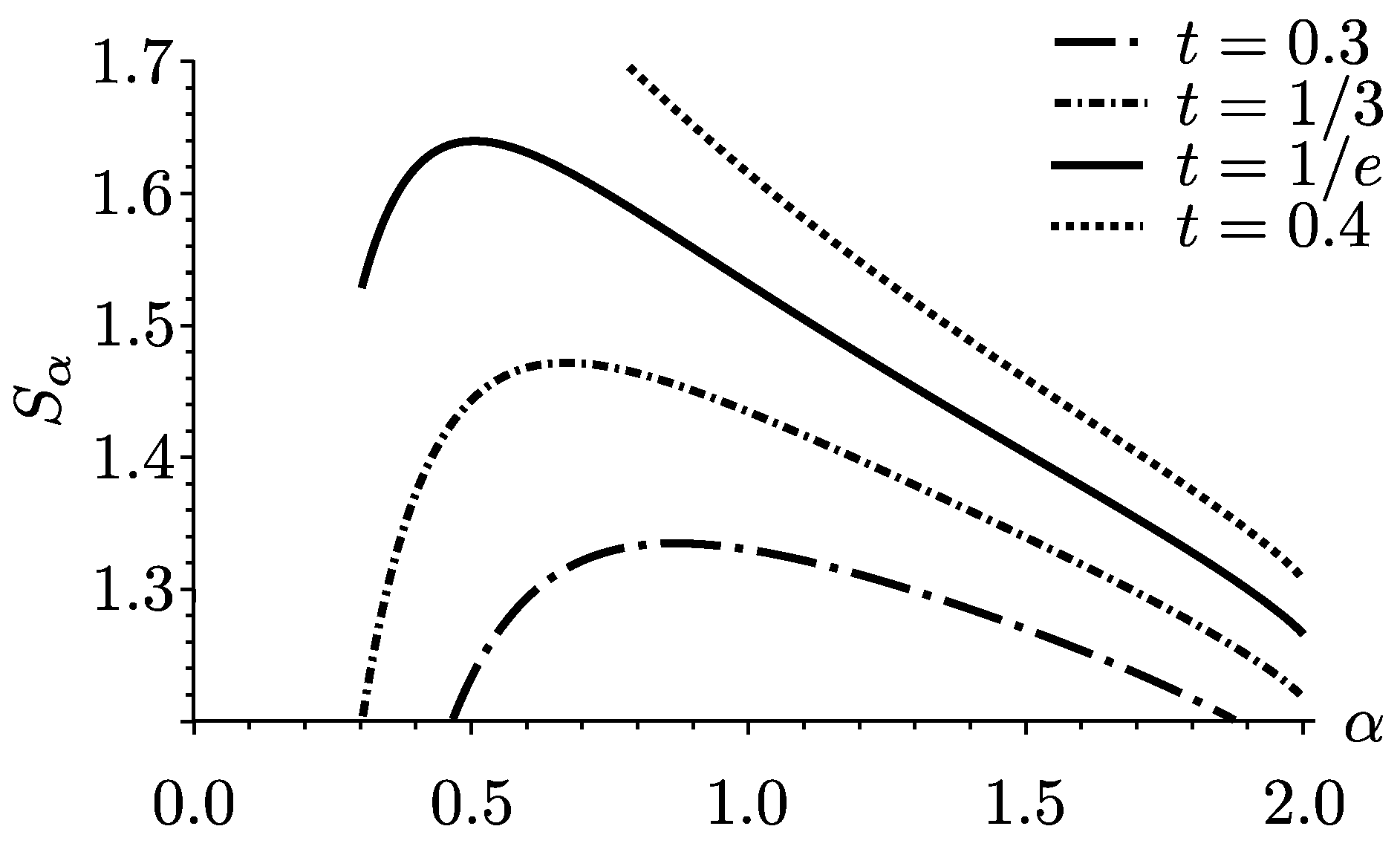With this as a guide, we find in Figure 5 that there is indeed a maximum in the computed interval.

There are however two important distinctions from the asymmetric cases. First, the scale of the function maximum in Figure 5 is small compared to the range of entropy values in Figure 3. Second, unlike the asymmetric cases, the maximum is transient—at least within the computed domain—confined to a narrow interval of time as the entropy transitions from monotonically increasing to monotonically decreasing. From an ordering perspective entropy works, excluding that narrow interval of time. In the asymmetric cases the difficulty was the persistence of an entropy maximum after a critical time that became the dominant feature of the function. It is possible that a maximum persists for very small values of α not computed.

From (16) the entropy production rate ${\dot{S}}_{\alpha }(t)$ is

$${\dot{S}}_{\alpha }(t)=1/(\alpha t),$$

(19)

which is the same as the asymmetric case, so it is positive and smallest for the Gaussian end of the regime. However unlike the asymmetric case, there is no propagation at the other end of the bridge.

5. Kullback–Leibler Entropy

Kullback–Leibler entropy (“Kullback” for short) [35,36] between two PDFs $P_a(x,t)$ and $P_b(x,t)$ is defined as

$$\begin{array}{c}\hfill K(P_a(x,t),P_b(x,t))={\int }_{-\infty }^{\infty }{P}_a(x,t)ln\left(\frac{P_a(x,t)}{P_b(x,t)}\right)\mathrm{d}x.\end{array}$$

(20)

We focus on comparing the Gaussian and the Cauchy distributions to particular reference distributions with $\alpha \in (0,2]$. Choosing $P_b=P_{\alpha }$ from (20) ensures integrals that are known to be convergent. $P_a$ will be given by the Gaussian distribution,

$$\begin{array}{cc}\hfill P_{\mathrm{G}}(x,t)& =\mathbf{S}\left(\left.x\right|2,0,\sqrt{t},0;0\right)=\mathcal{N}(0,2t)=\frac{1}{2\sqrt{\pi t}}exp\left(-\frac{x^2}{4t}\right),\hfill \end{array}$$

(21)

or the Cauchy distribution,

$$\begin{array}{cc}\hfill P_{\mathrm{C}}(x,t)& =\mathbf{S}\left(\left.x\right|1,0,t,0;0\right)=\frac{1}{\pi }\left(\frac{t}{x^2+t^2}\right).\hfill \end{array}$$

(22)

In the Gaussian case we have

$$\begin{array}{cc}\hfill K(P_{\mathrm{G}},P_{\alpha })& ={\int }_{-\infty }^{\infty }{P}_{\mathrm{G}}(x,t)ln\left(\frac{P_{\mathrm{G}}(x,t)}{P_{\alpha }(x,t)}\right)\mathrm{d}x\hfill \\ & ={\int }_{-\infty }^{\infty }{P}_{\mathrm{G}}(x,t)ln{P}_{\mathrm{G}}(x,t)\mathrm{d}x-{\int }_{-\infty }^{\infty }{P}_{\mathrm{G}}(x,t)ln{P}_{\alpha }(x,t)\mathrm{d}x\hfill \\ & =-1/2\left[1+ln\left(4\pi t\right)\right]+K^{†}(P_{\mathrm{G}},P_{\alpha }),\hfill \end{array}$$

(23)

where $K^{†}(P_{\mathrm{G}},P_{\alpha })$ is known as the cross entropy.

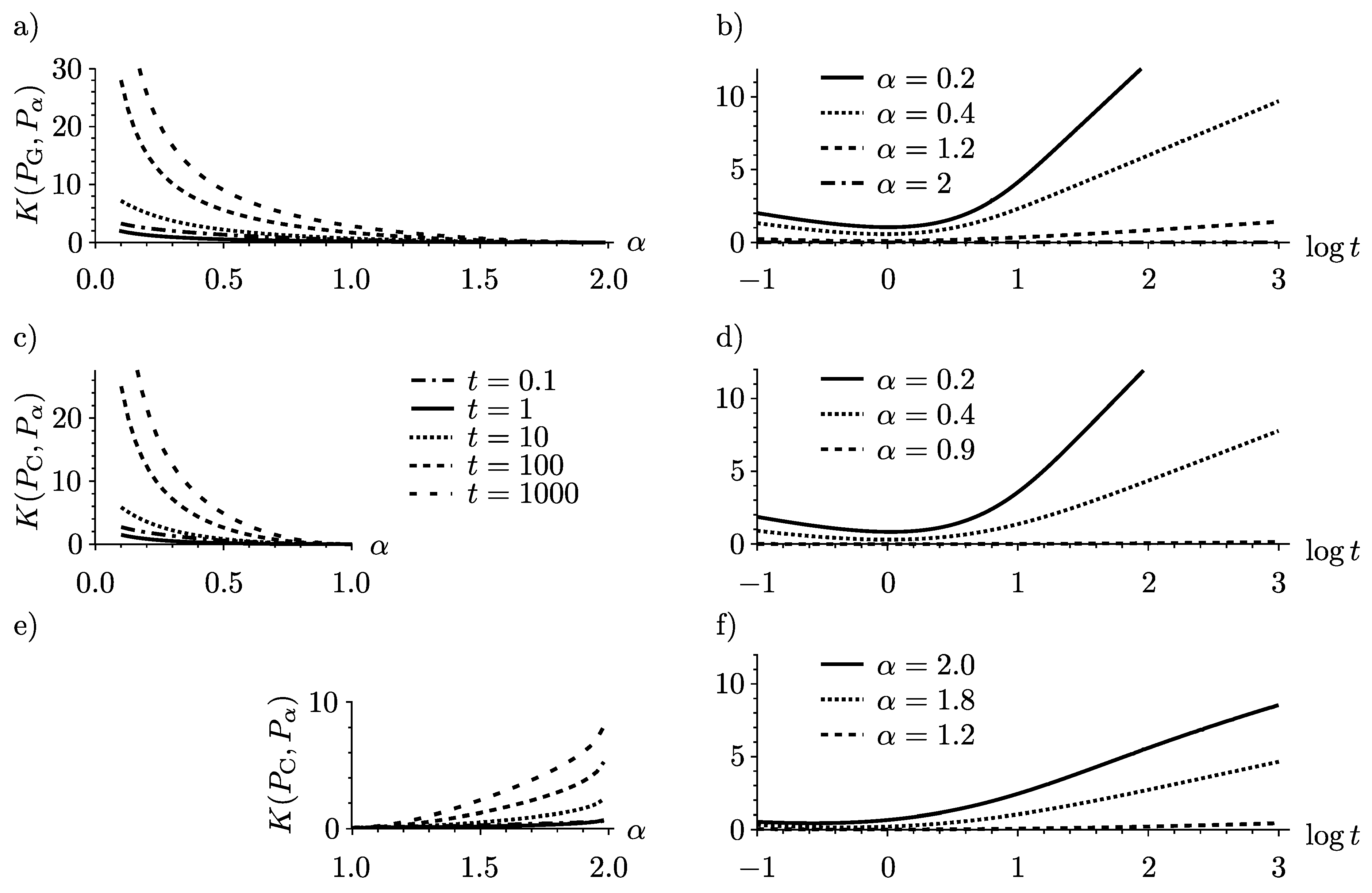
The resulting plots of the Kullback depending on α and on t are given in Figure 6. $K(P_{\mathrm{G}},P_{\alpha })$ is positive and monotonically decreasing with α. Moreover when α approaches 2, $P_{\alpha }$ approaches $P_{\mathrm{G}}$, so the Kullback needs to vanish for all times in that limit. For all $\alpha \in (0,2]$ the α-ordering is preserved for all times t as it is depicted in Figure 6.

Similar results are obtained for the Kullback with respect to the Cauchy distribution (22). In this case the Kullback is

$$\begin{array}{cc}\hfill K(P_{\mathrm{C}},P_{\alpha })& ={\int }_{-\infty }^{\infty }{P}_{\mathrm{C}}(x,t)ln\left(\frac{P_{\mathrm{C}}(x,t)}{P_{\alpha }(x,t)}\right)\mathrm{d}x.\hfill \end{array}$$

(24)

The numerical results for a wide range of times and values of α within the domain $(0,2]$ are depicted in Figure 6c–f. As the Cauchy distribution ($\alpha =1$) is in the middle of the domain $(0,2]$, the ordering behavior is split into two regimes. Within $(0,1]$ the Kullback decreases for increasing α, whereas for $[1,2]$ it increases from 0. Thus, the α-ordering for fixed time is separately preserved for both sub regimes $(0,1]$ and $[1,2]$. In addition in the $(0,1]$ segment, it is worth noting how similar the plot is to the Gaussian case. This is reinforced by the remarkable similarity of images Figure 6b and Figure 6d.

6. Conclusions

Previously we have examined bridging regimes between diffusion and waves. In those regimes the asymmetry of the resulting PDF produced a phenomenon of apparent movement called pseudo propagation that mapped onto normal mathematical propagation in the wave limit. The different rates of movement in space of features in the PDFs suggested distinctive internal tempos for each evolution equation in the regime, and was used to help make sense out of the peculiarities such as entropy having maxima in the regime between diffusion and waves. This paper aimed to control for pseudo propagation by employing a symmetric fractional derivative in an evolution equation with similar scaling properties. This yielded symmetric unimodal solutions in which the peak remains fixed in space, with all entropy production resulting from a sinking and spreading PDF, with no apparent spatial movement.

In the symmetric case the entropy production rate still increases as one moves away from the diffusion equation. This is consistent with the scaling properties of the symmetric fractional diffusion equation. However, this is no paradox in the sense that the opposite end of the regime $\alpha \to 0$ is not an evolution equation, let alone a diffusion equation. The entropy still shows a maximum over α despite symmetry, but it appears transient in terms of the computed domain and is in any case difficult to find unlike that of symmetric cases. This feature in the symmetric case means that entropy can be used to order systems moving away from the wave equation up to the end of the computed interval. But bear in mind there is no particular thermodynamic significance to this ordering, as $\alpha \to 0$ is not a reversible limit, but it does imply that the pseudo-propagation is important for these distinctive phenomena. It is not so surprising given the ordering property of entropy that the Kullback also preserved its ordering relationship in this case.

Additional features of significance emerged too. There are two sub-regimes split at $\alpha =1$. As α decreases well below 1 the PDFs become very highly peaked near zero, creating a negative core in the kernel of the entropy, accompanied by two maxima. This feature intensifies as α approaches 0, which is outside of the domain of consistent definition of the symmetric derivative as it has been constructed. This regime is computationally problematic and of interest for future exploration.

A limitation of this treatment is the presumption of unimodal symmetry. We envision a “twin peaks” approach to symmetry for future work. Also, in terms of future work a treatment of this domain in terms of extended entropies would be interesting, especially given recent work [37,38,39,40,41,42,43] in connection to this field.