Bivariate Partial Information Decomposition: The Optimization Perspective

Abstract

Bertschinger, Rauh, Olbrich, Jost, and Ay (Entropy, 2014) have proposed a definition of a decomposition of the mutual information $MI(\mathbf{X}:\mathbf{Y},\mathbf{Z})$ into shared, synergistic, and unique information by way of solving a convex optimization problem. In this paper, we discuss the solution of their Convex Program from theoretical and practical points of view.

1. Introduction

Bertschinger, Rauh, Olbrich, Jost, and Ay [1] have proposed to compute a decomposition of the mutual information $MI(\mathbf{X}:\mathbf{Y},\mathbf{Z})$ into shared, synergistic, and unique contributions by way of solving a convex optimization problem. It is important to mention that William and Beer in [2] were the first to propose a measure for information decomposition. That measure suffered from serious flaws, which prompted a series of other papers [3,4,5] trying to improve these results. Denote by X the range of the random variable $\mathbf{X}$, by Y the range of $\mathbf{Y}$, and by Z the range of $\mathbf{Z}$. Further, let

$$\begin{array}{ccc}\hfill b_{x,y}^{\mathtt{y}}& =\mathbb{P}\left(\mathbf{X}=x\wedge \mathbf{Y}=y\right)\hfill & \hspace{1em}\hspace{1em}\hspace{1em}\mathrm{for}\mathrm{all}x\in X,y\in Y\hfill \\ \hfill b_{x,z}^{\mathtt{z}}& =\mathbb{P}\left(\mathbf{X}=x\wedge \mathbf{Z}=z\right)\hfill & \hspace{1em}\hspace{1em}\hspace{1em}\mathrm{for}\mathrm{all}x\in X,y\in Y\hfill \end{array}$$

the marginals. Then the Bertschinger et al. definition of synergistic information is

$$\widetilde{\mathrm{C}\mathrm{I}}(\mathbf{X}:\mathbf{Y};\mathbf{Z}):=\mathrm{MI}(\mathbf{X}:\mathbf{Y},\mathbf{Z})-\underset{q}{\min }{\mathrm{MI}}_{(x,y,z)\sim q}(x:y,z),$$

where MI denotes mutual information, and $(x,y,z)\sim q$ stands for $(x,y,z)$ is distributed according to the probability distribution q. The minimum ranges over all probability distributions $q\in {[0,1]}^{X\times Y\times Z}$ which satisfy the marginal equations

$$\begin{array}{ccc}\hfill q_{x,y,\ast }& =b_{x,y}^{\mathtt{y}}\hfill & \hspace{1em}\hspace{1em}\hspace{1em}\mathrm{for}\mathrm{all}(x,y)\in X\times Y\hfill \\ \hfill q_{x,\ast ,z}& =b_{x,z}^{\mathtt{z}}\hfill & \hspace{1em}\hspace{1em}\hspace{1em}\mathrm{for}\mathrm{all}(x,z)\in X\times Z.\hfill \end{array}$$

We use the notational convention that an asterisk “∗” is to be read as “sum over everything that can be plugged in here”; e.g.,

$$q_{x,y,\ast }:=\sum _w{q}_{x,y,w}.$$

(We don’t use the symbol ∗ in any other context).

As pointed out in [1], the function $q\mapsto {\mathrm{MI}}_{(x,y,z)\sim q}(x:y,z)$ is convex and smooth in the interior of the convex region, and hence, by textbook results on convex optimization, for every $\epsilon >0$, an $\epsilon$-approximation of the optimum—i.e., a probability distribution $q^{★}$ for which ${\mathrm{MI}}_{(x,y,z)\sim q^{★}}(x:y,z)$ is at most $\epsilon$ larger than the minimum—can be found in at most $O({\alpha }^2/{\epsilon }^2)$ rounds of an iterative algorithm (e.g., Proposition 7.3.1 in [6]), with a parameter $\alpha$ (the asphericity of the feasible region) depending on the marginals $b^{\mathtt{y}}$, $b^{\mathtt{z}}$. Each iteration involves evaluating the gradient of ${\mathrm{MI}}_{(x,y,z)\sim q^{★}}(x:y,z)$ with respect to q, and $O\left(\left|X\times Y\times Z\right|\right)$ additional arithmetic operations.

In Appendix A of their paper, Bertschinger et al. discuss practical issues related to the solution of the convex optimization problem: They analyze the feasible region, solve by hand some of the problems, and complain that Mathematica could not solve the optimization problem out of the box.

Our paper is an expansion of that appendix in [1]. Driven by the need in application areas (e.g., [7]) to have a robust, fast, out-of-the-box method for computing $\widetilde{\mathrm{C}\mathrm{I}}$, we review the required convex optimization background; discuss different approaches to computing $\widetilde{\mathrm{C}\mathrm{I}}$ and the theoretical reasons contributing to the poor performance of some of them; and finally compare several of these approaches on practical problem instance. In conclusion, we offer two different practical ways of computing $\widetilde{\mathrm{C}\mathrm{I}}$.

The convex optimization problem in [1] is the following:

$$\begin{array}{ccc}\hfill \mathrm{minimize}& {\mathrm{MI}}_{(x,y,z)\sim q}(x:y,z)\hfill & \mathrm{over}q\in {\mathbb{R}}^{X\times Y\times Z}\hfill \\ \hfill \mathrm{subject}\mathrm{to}& q_{x,y,\ast }=b_{x,y}^{\mathtt{y}}\hfill & \mathrm{for}\mathrm{all}(x,y)\in X\times Y\hfill \\ \hfill & q_{x,\ast ,z}=b_{x,z}^{\mathtt{z}}\hfill & \mathrm{for}\mathrm{all}(x,z)\in X\times Z\hfill \\ \hfill & q_{x,y,z}\ge 0\hfill & \mathrm{for}\mathrm{all}(x,y,z)\in X\times Y\times Z\hfill \end{array}$$

This is a Convex Program with a non-linear, convex continuous objective function $q\mapsto {\mathrm{MI}}_{(x,y,z)\sim q}(x:y,z)$, which is smooth in all points q with no zero entry. The feasible region (i.e., the set of all q satisfying the constraints) is a compact convex polyhedron, which is nonempty, as the distribution of the original random variables $(\mathbf{X},\mathbf{Y},\mathbf{Z})$ is a feasible solution. Clearly, the condition that q should be a probability distribution is implied by it satisfying the marginal equations.

In the next section, we review some background about convex functions and convex optimization, in particular with respect to non-smooth functions. Section 3 aims to shed light on the theoretical properties of the convex program (CP). In Section 4, we present the computer experiments which we conducted and their results. Some result tables are in the Appendix A.

2. Convex Optimization Basics

Since the target audience of this paper is not the optimization community, for the sake of easy reference, we briefly review the relevant definitions and facts, tailored for our problem: the feasible region is polyhedral, the objective function is (convex and continuous but) not everywhere smooth.

Let f be a convex function defined on a convex set $C\subseteq {\mathbb{R}}^n$; let $x\in C$ and $d\in {\mathbb{R}}^n$. The directional derivative of f at x in the direction of d is defined as the limit

$${\displaystyle f^{\prime }(x;d):=\underset{\epsilon \searrow 0}{\lim }\frac{f(x+\epsilon d)-f\left(x\right)}{\epsilon }\in [-\infty ,\infty ].}$$

(1)

Remark 1

([8], Lemma 2.71). The limit in (1) exists in $[-\infty ,\infty ]$, by the convexity of f.

A subgradient of f at a point $x\in C$ is a vector $g\in {\mathbb{R}}^n$ such that, for all $y\in C$, we have $f\left(y\right)\ge f\left(x\right)+g^{⏉}(y-x)$.

There can be many subgradients of f at a point. However:

Remark 2.

If f is differentiable at x, then $\nabla f\left(x\right)$ is the only subgradient of f at x.

Lemma 1

([8], Lemma 2.73). If g is a subgradient of f at $x\in C$, and $y\in C$, then $g^{⏉}(y-x)\le f^{\prime }(x;y-x)$.

We state the following lemma for convenience (it will be used in the proof of Proposition 2). It is a simplification of the Moreau-Rockafellar Theorem ([8], Theorem 2.85).

Lemma 2.

Let $C_i\subset {\mathbb{R}}^{\ell }$, $i=1,\cdots ,k$ be a closed convex sets, $f_i:C_i\to \mathbb{R}$ continuous convex functions, and

$$f\left(x\right)=\sum _{i=1}^k{f}_i\left(x_i\right)$$

for $x=(x_1,\cdots ,x_k)\in {\prod }_{i=1}^k{C}_i\subset \mathbb{R}{{(}^{\ell })}^k$. If, for $i=1,\cdots ,k$, $g_i$ is a subgradient of $f_i$ at $x_i$, then $g:=(g_1,\cdots ,g_k)$ is a subgradient of f at x. Moreover, all subgradients of f at x are of this form.

For the remainder of this section, we reduce the consideration to convex sets C of the form given in the optimization problem (CP). Let A be an $m\times n$ matrix, and b an m-vector. Assume that $C=\{x\in {\mathbb{R}}^n\mid Ax=b\wedge x\ge 0\}$. Suppose f is a convex function defined on C. Consider the convex optimization problem ${\displaystyle \underset{x\in C}{\min }f\left(x\right)}$.

Let $x\in C$. A vector $d\in {\mathbb{R}}^n$ is called a feasible descent direction of f at x, if

(a)

for some $\epsilon >0$, $x+\epsilon d\in C$ (“feasible direction”); and

(b)

$f^{\prime }(x;d)<0$ (“descent direction”).

Clearly, if a feasible descent direction of f at x exists, then x is not a minimum of f over C. The following theorem is a direct consequence of ([8], Theorem 3.34) adapted to our situation.

Theorem 1 (Karush-Kuhn-Tucker).

Suppose that for every $j=1,\cdots ,n$, there is an $x\in C$ with $x_j>0$. The function f attains a minimum over C at a point $x\in C$ if, and only if, there exist

• a subgradient g of f at x
• and an m-vector $\lambda \in {\mathbb{R}}^m$

such that ${\displaystyle A^{⏉}\lambda \le g}$, and for all $j\in \{1,\cdots ,n\}$ with $x_j>0$, equality holds: ${\displaystyle {(A^{⏉}\lambda )}_j=g_j}$.

The condition “$x_j=0$ or ${(A^{⏉}\lambda )}_j=g_j$” is called complementarity.

2.1. Convex Optimization Through Interior Point Methods

For reasons which will become clear in Section 3, it is reasonable to try to solve (CP) using a so-called Interior Point or Barrier Method (we gloss over the (subtle) distinction between IPMs and BMs). The basic idea of these iterative methods is that all iterates are in the “interior” of something. We sketch what goes on.

From a theoretical point of view, a closed convex set C is given in terms of a barrier function, i.e., a convex function $F:C\to \mathbb{R}$ with $F\left(x\right)\to \infty$ whenever x approaches the boundary of C. The prototypical example is $C:={\left[0,\infty \right]}^n$, and $F\left(x\right):=-{\sum }_j\ln x_j$. The goal is to minimize a linear objective function $x\mapsto {\sum }_j{c}_j{x}_j$ over C.

To fit problems with nonlinear (convex) objective f into this paradigm, the “epigraph form” is used, which means that a new variable s is added along with a constraint $f\left(q\right)\le s$, and the objective is “minimize s”.

The algorithm maintains a barrier parameter $t>0$, which is increased gradually. In iteration k, it solves the unconstrained optimization problem

$$x^{\left(k\right)}:=\underset{x\in {\mathbb{R}}^n}{\mathrm{argmin}}\left(t_k·c^{⏉}x+F\left(x\right)\right)$$

(2)

The barrier parameter is then increased, and the algorithm proceeds with the next iteration. The fact that the barrier function tends to infinity towards the boundary of C makes sure that the iterates $x^{\left(k\right)}$ stay in the interior of C for all k.

The unconstrained optimization problem (2) is solved using Newton’s method, which is itself iterative. If x is the current iterate, Newton’s method finds the minimum to the second order Taylor expansion about x of the objective function $g:x\mapsto t_k·c^{⏉}x+F\left(x\right)$:

$$\begin{array}{c}\underset{y\in {\mathbb{R}}^n}{\mathrm{argmin}}\left(g\left(x\right)+\nabla g{\left(x\right)}^{⏉}(y-x)+\frac{1}{2}(y-x)Hg\left(x\right)(y-x)\right)\hfill \\ =x-Hg{\left(x\right)}^{-1}\nabla g\left(x\right).\hfill \end{array}$$

where $Hg\left(x\right)$ denotes the Hessian of g at x. Then Newton’s method updates x (e.g., by simply replacing it with the argmin).

Note that $Hg\left(x\right)=HF\left(x\right)$, so the convergence properties (as well as, whether it works at all or not), depend on the properties of the barrier function. Suitable barrier functions are known to exist for all compact convex sets [9,10]. However, for a given set, finding one which can be quickly evaluated (along with the gradient and the Hessian) is sometimes a challenge.

A more “concrete” point of view is the following. Consider f and C as above: $C:=\{x\mid Ax=b,x\ge 0\}$ and f is convex and continuous on C, and smooth in the interior of C (here: the points $x\in C$ with $x_j>0$ for all j) which we assume to be non-empty. A simple barrier-type algorithm is the following. In iteration k, solve the equality-constrained optimization problem

$$x^{\left(k\right)}:=\underset{\begin{array}{c}x\in {\mathbb{R}}^n\\ Ax=b\end{array}}{\mathrm{argmin}}\left(t_k·f\left(x\right)-\sum _{j=1}^n\ln \left(x_j\right)\right).$$

(3)

The equality-constrained problem is solved by a variant of Newton’s method: If x is the current iterate, Newton’s method finds the minimum to the second order Taylor expansion about x of the function $g:x\mapsto t_{k}f\left(x\right)-\sum \ln \left(x_j\right)$ subject to the equations $Ax=b$, using Lagrange multipliers, i.e., it solves the linear system

$$\begin{array}{cc}\hfill Hg\left(x\right)y+A^{⏉}\lambda & =-\nabla g\left(x\right)\hfill \\ \hfill Ax& =b,\hfill \end{array}$$

with $Hg\left(x\right)=t_{k}Hf\left(x\right)+{\mathrm{Diag}}_j(1/x_j^2)$ and $\nabla g\left(x\right)=t_k\nabla f\left(x\right)-{\mathrm{Diag}}_j(1/x_j)$, where $Diag(·)$ denotes a diagonal matrix of appropriate size with the given diagonal.

By convexity of f, $Hf\left(x\right)$ is positive semidefinite, so that adding the diagonal matrix results in a (strictly) positive definite matrix. Hence, the system of linear equations always has a solution.

The convergence properties of this simple barrier method now depend on properties of f. We refer the interested reader to ([11], Chapter 11) for the details.

Generally speaking, today’s practical Interior Point Methods are “Primal-Dual Interior Point Methods”: They solve the “primal” optimization problem and the dual—the system in Theorem 1—simultaneously. After (successful) termination, they return not only an $\epsilon$-approximation x of the optimum, but also the Lagrange multipliers $\lambda$ which certify optimality.

3. Theoretical View on Bertschinger et al.’s Convex Program

We will use the following running example in this section.

Example 1 (Part 1/4).

Let $X:=\{$0, 1, 2, 3}, $Y,Z:=\{$0, 1}.

$$\begin{array}{cccc}{b}_{0,0}^{\mathtt{y}}:=1/4\hfill & b_{0,1}^{\mathtt{y}}:=0\hfill & b_{0,0}^{\mathtt{z}}:=1/4\hfill & b_{0,1}^{\mathtt{z}}:=0\hfill \\ b_{1,0}^{\mathtt{y}}:=0\hfill & b_{1,1}^{\mathtt{y}}:=1/4\hfill & b_{1,0}^{\mathtt{z}}:=0\hfill & b_{1,1}^{\mathtt{z}}:=1/4\hfill \\ b_{2,0}^{\mathtt{y}}:=1/8\hfill & b_{2,1}^{\mathtt{y}}:=1/8\hfill & b_{2,0}^{\mathtt{z}}:=1/8\hfill & b_{2,1}^{\mathtt{z}}:=1/8\hfill \\ b_{3,0}^{\mathtt{y}}:=1/8\hfill & b_{3,1}^{\mathtt{y}}:=1/8\hfill & b_{3,0}^{\mathtt{z}}:=1/8\hfill & b_{3,1}^{\mathtt{z}}:=1/8\hfill \end{array}$$

Among all $q\in {\mathbb{R}}^{X\times Y\times Z}$ (16 dimensions) satisfying the 16 equations

$$\begin{array}{cccc}\hfill q_{x,y,\ast }& =b_{x,y}^{\mathtt{y}}\forall x,y,\hfill & \hspace{1em}\hspace{1em}\hspace{1em}\hfill q_{x,\ast ,z}& =b_{x,z}^{\mathtt{z}}\forall x,z,\hfill \end{array}$$

and the 16 inequalities $q_{x,y,z}\ge 0$ for all $x,y,z$, we want to find one which minimizes ${\mathrm{MI}}_{(x,y,z)\sim q}(x:y,z)$.

3.1. The Feasible Region

In this section, we discuss the feasible region:

$$\P \left(b\right):=\left\{q\in {\mathbb{R}}_{+}^{X\times Y\times Z}|\forall x,y,z:q_{x,y,\ast }=b_{x,y}^{\mathtt{y}}\&q_{x,\ast ,z}=b_{x,z}^{\mathtt{z}}\right\}$$

We will omit the “$\left(b\right)$” when no confusion can arise. We will always make the following assumptions:

• $b^{\mathtt{y}}$ and $b^{\mathtt{z}}$ are probability distributions.
• $\P \left(b\right)$ is non-empty. This is equivalent to $b_{x,\ast }^{\mathtt{y}}=b_{x,\ast }^{\mathtt{z}}$ for all $x\in X$.
• No element of X is “redundant”, i.e., for every $x\in X$ we have both $b_{x,\ast }^{\mathtt{y}}>0$ and $b_{x,\ast }^{\mathtt{z}}>0$.

First of all, recall the vectors $\overline{d}\in {\mathbb{R}}^{X\times Y\times Z}$ from Appendix A.1 of [1], defined by

$${\overline{d}}^{x,y,z,y^{\prime },z^{\prime }}:=1^{x,y,z}+1^{x,y^{\prime },z^{\prime }}-1^{x,y,z^{\prime }}-1^{x,y^{\prime },z},$$

(4)

(where $1\cdots$ is the vector with exactly one non-zero entry in the given position, and 0 otherwise) satisfy ${\overline{d}}_{x,y,\ast }={\overline{d}}_{x,\ast ,z}=0$ for all $x,y,z$ (we omit the superscripts for convenience, when possible).

Our first proposition identifies the triples $(x,y,z)$ for which the equation $q_{x,y,z}=0$ holds for all $q\in \P \left(b\right)$.

Proposition 1.

If $q_{x,y,z}=0$ holds for all $q\in \P \left(b\right)$, then $b_{x,y}^{\mathtt{y}}=0$ or $b_{x,z}^{\mathtt{z}}=0$.

Proof. 

Let $x,y,z\in X\times Y\times Z$, and assume that $b_{x,y}^{\mathtt{y}}\ne 0$ and $b_{x,z}^{\mathtt{z}}\ne 0$. Take any $p\in \P \left(b\right)$ with $p_{x,y,z}=0$—if no such p exists, we are done. Since the marginals are not zero, there exist $y^{\prime }\in Y\backslash \left\{y\right\}$ and $z^{\prime }\in Z\backslash \left\{z\right\}$ with $p_{x,y^{\prime },z}>0$ and $p_{x,y,z^{\prime }}>0$. Let $\overline{d}:={\overline{d}}^{x,y,z,y^{\prime },z^{\prime }}$. By the remarks preceding the proposition, $p+\delta \overline{d}$ satisfies the marginal equations for all $\delta \in \mathbb{R}$. Since $p_{x,y^{\prime },z}>0$ and $p_{x,y,z^{\prime }}>0$, there exists a $\delta >0$ such that $q:=p+\delta \overline{d}\ge 0$. Hence, we have $q\in \P \left(b\right)$ and $q_{x,y,z}>0$, proving that the equation $q_{x,y,z}=0$ is not satisfied by all elements of $\P \left(b\right)$. ☐

The proposition allows us to restrict the set of variables of the Convex Program to those triples $(x,y,z)$ for which a feasible q exists with $q_{x,y,z}\ne 0$ (thereby avoiding unneccessary complications in the computation of the objective function and derivatives; see the next section); the equations with RHS 0 become superfluous. We let

$$\mathcal{J}\left(b\right):=\left\{(x,y,z)\in X\times Y\times Z|b_{x,y}^{\mathtt{y}}>0\wedge b_{x,z}^{\mathtt{z}}>0\right\}$$

(5)

denote the set of remaining triplets. We will omit the “$\left(b\right)$” when no confusion can arise.

Example 2 (Part 2/4).

Continuing Example 1, we see that the equations with RHS 0 allow to omit the variables $q_{x,y,z}$ for the following triples $(x,y,z)$:

$$\begin{array}{cc}(0,1,0)& (0,0,1)\\ (0,1,1)& (0,1,1)\\ (1,0,0)& (1,0,0)\\ (1,0,1)& (1,1,0)\end{array}$$

Hence, $\mathcal{J}:=\left\{\right($0, 0, 0$),($1, 1, 1$),($2$,y,z),($3$,y^{\prime },z^{\prime })\mid y,z,y^{\prime },z^{\prime }\in \{$0, 1$\left\}\right\}$ (10 variables), and we are left with the following 12 equations:

$$\begin{array}{cccc}{q}_{0,0,\ast }=b_{0,0}^{\mathtt{y}}=1/4& & q_{0,\ast ,0}=b_{0,0}^{\mathtt{z}}=1/4& \\ & q_{1,1,\ast }=b_{1,1}^{\mathtt{y}}=1/4& & q_{1,\ast ,1}=b_{1,1}^{\mathtt{z}}=1/4\\ q_{2,0,\ast }=b_{2,0}^{\mathtt{y}}=1/8& q_{2,1,\ast }=b_{2,1}^{\mathtt{y}}=1/8& q_{2,\ast ,0}=b_{2,0}^{\mathtt{z}}=1/8& q_{2,\ast ,1}=b_{2,1}^{\mathtt{z}}=1/8\\ q_{3,0,\ast }=b_{3,0}^{\mathtt{y}}=1/8& q_{3,1,\ast }=b_{3,1}^{\mathtt{y}}=1/8& q_{3,\ast ,0}=b_{3,0}^{\mathtt{z}}=1/8& q_{3,\ast ,1}=b_{3,1}^{\mathtt{z}}=1/8.\end{array}$$

We can now give an easy expression for the dimension of the feasible region (with respect to the number of variables, $\left|\mathcal{J}\left(b\right)\right|$).

Corollary 1.

The dimension of $\P \left(b\right)$ is

$$\left|\mathcal{J}\left(b\right)\right|+\left|X\right|-\left|\{(x,y)\mid b_{x,y}^{\mathtt{y}}>0\}\right|-\left|\{(x,z)\mid b_{x,z}^{\mathtt{z}}>0\}\right|.$$

Proof. 

For $x\in X$, the set $Y_x:=\{y\in Y\mid b_{x,y}^{\mathtt{y}}>0\}$ is non-empty, by assumption 3; the same is true for $Z_x:=\{z\in Z\mid b_{x,z}^{\mathtt{z}}>0\}$. Note that $\mathcal{J}\left(b\right)$ is the disjoint union of the sets $\left\{x\right\}\times Y_x\times Z_x$, $x\in X$.

Lemmas 26 and 27 of [1] now basically complete the proof of our corollary: It implies that the dimension is equal to

$$\sum _{x\in X}(\left|Y_x\right|-1)(\left|Z_x\right|-1).$$

As $\mathcal{J}\left(b\right)$ is the disjoint union of the sets $\left\{x\right\}\times Y_x\times Z_x$, $x\in X$, we find this quantity to be equal to

$$\left|\mathcal{J}\left(b\right)\right|+\left|X\right|-\sum _{x\in X}\left(\left|Y_x\right|+\left|Z_x\right|\right).$$

Finally,

$$\sum _{x\in X}\left(\left|Y_x\right|+\left|Z_x\right|\right)=\left|\{(x,y)\mid b_{x,y}^{\mathtt{y}}>0\}\right|+\left|\{(x,z)\mid b_{x,z}^{\mathtt{z}}>0\}\right|,$$

which concludes the proof of the corollary. ☐

Example 3 (Part 3/4).

Continuing Example 1, we find that the values for the variables $q_{0,0,0}$ and $q_{1,1,1}$ are fixed to 1/4, whereas each of two sets of four variables $q_{2,y,z}$, $y,z\in \{$0, 1}, and $q_{3,y,z}$, $y,z\in \{$0, 1}, offers one degree of freedom, so the dimension should be 2. And indeed: $\left|\mathcal{J}\right|+\left|X\right|-\left|\{(x,y)\mid b_{x,y}^{\mathtt{y}}>0\}\right|-\left|\{(x,z)\mid b_{x,z}^{\mathtt{z}}>0\}\right|=10+4-12=2$.

3.2. The Objective Function and Optimality

We now discuss the objective function. The goal is to minimize

$${\mathrm{MI}}_{(x,y,z)\sim q}(x:y,z)=H_{(x,y,z)\sim q}\left(x\right)-H_{(x,y,z)\sim q}(x\mid y,z).$$

Since the distribution of x is fixed by the marginal equations, the first term in the sum is a constant, and we are left with minimizing negative conditional entropy. We start by discussing negative conditional entropy as a function on its full domain (We don’t assume q to be a probability distrbution, let alone to satisfy the marginal equations): f: ${\mathbb{R}}_{+}^{\mathcal{J}}\to \mathbb{R}$ (with $\mathcal{J}=\mathcal{J}\left(b\right)$ for arbitrary but fixed b)

$$f:q\mapsto \sum _{(x,y,z)\in \mathcal{J}}{q}_{x,y,z}\ln \left(\frac{q_{x,y,z}}{q_{\ast ,y,z}}\right),$$

(6)

where we set $0\ln (\cdots )$ := 0, as usual. The function f is continuous on its domain, and it is smooth on ${[0,\infty ]}^{\mathcal{J}}$. Indeed, we have the gradient

$${\left(\nabla f\left(q\right)\right)}_{x,y,z}={\partial }_{x,y,z}f\left(q\right)=\ln \left(\frac{q_{x,y,z}}{q_{\ast ,y,z}}\right),$$

(7)

and the Hessian

$${\left(Hf\left(q\right)\right)}_{(x,y,z),(x^{\prime },y^{\prime },z^{\prime })}={\partial }_{x,y,z}{\partial }_{x^{\prime },y^{\prime },z^{\prime }}f\left(q\right)=\left\{\begin{array}{cc}{\displaystyle 0,}\hfill & \mathrm{if}(y^{\prime },z^{\prime })\ne (y,z)\hfill \\ {\displaystyle \frac{-1}{q_{\ast ,y,z}},}\hfill & \mathrm{if}(y^{\prime },z^{\prime })=(y,z),x\ne x^{\prime }\hfill \\ {\displaystyle \frac{q_{\ast ,y,z}-q_{x,y,z}}{q_{x,y,z}{q}_{\ast ,y,z}},}\hfill & \mathrm{if}(x^{\prime },y^{\prime },z^{\prime })=(x,y,z).\hfill \end{array}\right.$$

(8)

It is worth pointing out that the Hessian, while positive semidefinite, is not positive definite, and, more pertinently, it is not in general positive definite on the tangent space of the feasible region, i.e., $r^{⏉}Hf\left(q\right)r=0$ is possible for $r\in {\mathbb{R}}^{\mathcal{J}}$ with $r(x,y,\ast )=r(x,\ast ,z)=0$ for all $(x,y,z).$ Indeed, if, e.g., $\mathcal{J}=X\times Y\times Z,$ it is easy to see the kernel of $Hf\left(q\right)$ has dimension $\left|Y\times Z\right|$, whereas the feasible region has dimension $\left|X\right|(\left|Y\right|-1)(\left|Z\right|-1)=\left|X\times Y\times Z\right|-\left|X\right|\left|Y\right|-\left|X\right|\left|Z\right|+1.$ Hence, if $\left|Y\times Z\right|>\left|X\right|\left|Y\right|+\left|X\right|\left|Z\right|-1$, then for every $q(!)$ the kernel of $Hf\left(q\right)$ the must have a non-empty intersection with the tangent space of the feasible region.

Optimality condition and boundary issues. In the case of points q which lie on the boundary of the domain, i.e., $q_{x,y,z}=0$ for at least one triplet $x,y,z$, some partial derivatives don’t exist. For $y,z$, denote $X_{yz}:=\left\{x\right|(x,y,z)\in \mathcal{J}\}$. The situation is as follows.

Proposition 2.

Let $q\in \P$.

(a) 

If there is a $(x,y,z)\in \mathcal{J}$ with $q_{x,y,z}=0$ but $q_{\ast ,y,z}>0$, the f does not have a subgradient at q. Indeed, there is a feasible descent direction of f at q with directional derivative $-\infty$.

(b) 

Otherwise—i.e., for all $(x,y,z)\in \mathcal{J}$, $q_{x,y,z}=0$ only if $q_{\ast ,y,z}=0$—subgradients exist. For all $y,z$, let ${\varrho }^{y,z}\in {[0,1]}^{X_{yz}}$ be a probability distribution on $X_{yz}$. Suppose that, for all $y,z$ with $q_{\ast ,y,z}>0$,

$${\varrho }_x^{y,z}=\frac{q_{x,y,z}}{q_{\ast ,y,z}}\mathit{for}\mathit{all}x\in X_{yz}.$$

(9)

Then g defined by $g_{x,y,z}:=\ln \left({\varrho }_x^{y,z}\right)$, for all $(x,y,z)\in \mathcal{J}$, is a subgradient of f at q.

Moreover, $g^{\prime }$ is a subgradient iff there exists such a g with

• $g_{x,y,z}^{\prime }\le g$ for all $(x,y,z)\in \mathcal{J}$ with $q_{x,y,z}=0$;
• $g_{x,y,z}^{\prime }=g$ for all $(x,y,z)\in \mathcal{J}$ with $q_{x,y,z}>0$;

Proof. 

For Proposition 2, let $(y,z)\in Y\times Z$ with $q_{\ast ,y,z}>0$, and $x\in X_{yz}$ with $q_{x,y,z}=0$. There exist $y^{\prime },z^{\prime }$ such that $q_{x,y^{\prime },z},q_{x,y,z^{\prime }}>0$. This means that $\overline{d}:={\overline{d}}^{x,y,z,y^{\prime },z^{\prime }}$ as defined in (4) is a feasible direction. Direct calculations (written down in [12]) show that $f^{\prime }(q;\overline{d})=-\infty$. Invoking Lemma 1 yields non-existence of the subgradient.

As to Proposition 2, we prove the statement for every pair $(y,z)\in Y\times Z$ for the function

$$f_{yz}:{\mathbb{R}}_{+}^{X_{yz}}\to \mathbb{R}:q\mapsto \sum _{x\in X_{yz}}{q}_x\ln (q_x/q_{\ast }),$$

and then use Lemma 2.

Let us fix one pair $(y,z)$. If $q_{x,y,z}>0$ for all $x\in X_{yz}$ holds, then we $f_{y,z}$ is differentiable at q, so we simply apply Remark 2.

Now assume $q_{\ast ,y,z}=0$. A vector $g\in {\mathbb{R}}^{X_{yz}}$ is a subgradient of $f_{yz}$, iff

$$\sum _{x\in X_{yz}}{r}_{x,y,z}\ln (r_{x,y,z}/r_{\ast ,y,z})=f_{yz}(q+r)\stackrel{!}{\ge }{f}_{yz}\left(q\right)+g^{⏉}r=f_{yz}\left(q\right)+\sum _{x\in X_{yz}}{r}_x{g}_x$$

(10)

holds for all $r\in {\mathbb{R}}^{\mathcal{J}}$ with $r_{x,y,z}\ge$ for all $(x,y,z)\in \mathcal{J}$, and $r_{\ast }>0$.

We immediately deduce $g_x\le 0$ for all x. Let ${\varrho }_x^{\prime }:=e^{gx}$ for all x, and ${\varrho }_x:={\varrho }_x^{\prime }/C$, with $C:={\varrho }_{\ast }^{\prime }$. Clearly $\varrho$ is a probability distribution on $X_{yz}$. Moreover, the difference LHS-RHS of (10) is equal to

$$D_{\mathrm{KL}}(r/r_{\ast }\parallel \rho )+\ln C,$$

with $D_{\mathrm{KL}}$ denoting Kullback-Leibler divergence. From the usual properties of the Kullback-Leibler divergence, we see that this expression is greater-than-or-equal to 0 for all r, if and only if $C>1$, which translates to

$$\sum _x{e}^{gx}\le 1.$$

From this, the statements in Proposition 2 follow. ☐

From the proposition, we derive the following corollary.

Corollary 2.

Suppose a minimum of f over $\P \left(b\right)$ is attained in a point q with $q_{x,y,z}=0$ for a triple $(x,y,z)$ with $b_{x,y}^{\mathtt{y}}>0$ and $b_{x,z}^{\mathtt{z}}>0$. Then $q_{u,y,z}=0$ for all $u\in X$.

Proof. 

This follows immediately from the fact, expressed in item Proposition 2 of the lemma, that a negative feasible descent direction exists at a point q which with $q_{x,y,z}=0$ for a triple $(x,y,z)\in \mathcal{J}\left(b\right)$ with $q_{\ast ,y,z}>0$. ☐

Based on Proposition 2 and the Karush-Kuhn-Tucker conditions, Theorem 1, we can now write down the optimality condition.

Corollary 3.

Let $q\in \P \left(b\right)$. The minimum of f over $\P \left(b\right)$ is attained in q if, and only if, (a) $q_{\ast ,y,z}=0$ holds whenever there is an $(x,y,z)\in \mathcal{J}\left(b\right)$ with $q_{x,y,z}=0$; and (b) there exist

• ${\lambda }_{x,y}\in \mathbb{R}$, for each $(x,y)$ with $b_{x,y}^{\mathtt{y}}>0$;
• ${\mu }_{x,z}\in \mathbb{R}$, for each $(x,z)$ with $b_{x,z}^{\mathtt{z}}>0$;

satisfying the following: For all $y,z$ with $q_{\ast ,y,z}>0$,

$$\begin{array}{cc}\hfill {\lambda }_{x,y}+{\mu }_{x,z}& =\ln \left(\frac{q_{x,y,z}}{q_{\ast ,y,z}}\right)\mathit{holds}\mathit{for}\mathit{all}x\in X_{yz};\hfill \end{array}$$

for all $y,z$ with $q_{\ast ,y,z}=0$ (but $X_{yz}\ne \varnothing$), there is a probability distribution $\varrho \in {\left[0,1\right]}^{X_{yz}}$ on $X_{yz}$ such that

$$\begin{array}{cc}\hfill {\lambda }_{x,y}+{\mu }_{x,z}& \le \ln \left({\varrho }_x^{y,z}\right)\mathit{holds}\mathit{for}\mathit{all}x\in X_{yz}.\hfill \end{array}$$

Example 4 (Part 4/4).

Continuing Example 1, let us now find the optimal solution “by hand”. First of all, note that $q_{0,0,0}=1/4=q_{1,1,1}$ holds for all feasible solutions. By Corollary 2, if q is an optimal solution, since $q_{0,0,0}>0$, we must have $q_{x,0,0}>0$ for $x=$ 2, 3; and similarly, $q_{x,1,1}>0$ for x = 2, 3.

To verify whether or not a given q is optimal, we have to find solutions ${\lambda }_{x,y}$, ${\mu }_{x,z}$ to the following system of equations and/or inequalities:

$$\begin{array}{cc}\hfill {\lambda }_{0,0}+{\mu }_{0,0}& =\ln (1/4/(1/4+q_{2,0,0}+q_{3,0,0}))\hfill \\ \hfill {\lambda }_{2,0}+{\mu }_{2,0}& =\ln (q_{2,0,0}/(1/4+q_{2,0,0}+q_{3,0,0}))\hfill \\ \hfill {\lambda }_{3,0}+{\mu }_{3,0}& =\ln (q_{3,0,0}/(1/4+q_{2,0,0}+q_{3,0,0}))\hfill \\ \hfill {\lambda }_{2,0}+{\mu }_{2,1}& \left\{\begin{array}{cc}=\ln (q_{2,0,1}/(q_{2,0,1}+q_{3,0,1})),\hfill & \mathit{if}{q}_{\ast ,0,1}>0\hfill \\ \le \ln \left({\varrho }_2^{01}\right),\hfill & \mathit{if}{q}_{\ast ,0,1}=0\hfill \end{array}\right.\hfill \\ \hfill {\lambda }_{3,0}+{\mu }_{3,1}& \left\{\begin{array}{cc}=\ln (q_{3,0,1}/(q_{2,0,1}+q_{3,0,1})),\hfill & \mathit{if}{q}_{\ast ,0,1}>0\hfill \\ \le \ln \left({\varrho }_3^{01}\right),\hfill & \mathit{if}{q}_{\ast ,0,1}=0\hfill \end{array}\right.\hfill \\ \hfill {\lambda }_{2,1}+{\mu }_{2,0}& \left\{\begin{array}{cc}=\ln (q_{3,1,0}/(q_{2,1,0}+q_{3,1,0})),\hfill & \mathit{if}{q}_{\ast ,1,0}>0\hfill \\ \le \ln \left({\varrho }_2^{10}\right),\hfill & \mathit{if}{q}_{\ast ,1,0}=0\hfill \end{array}\right.\hfill \\ \hfill {\lambda }_{3,1}+{\mu }_{3,0}& \left\{\begin{array}{cc}=\ln (q_{3,1,0}/(q_{2,1,0}+q_{3,1,0})),\hfill & \mathit{if}{q}_{\ast ,1,0}>0\hfill \\ \le \ln \left({\varrho }_3^{10}\right),\hfill & \mathit{if}{q}_{\ast ,1,0}=0\hfill \end{array}\right.\hfill \\ \hfill {\lambda }_{1,1}+{\mu }_{1,1}& =\ln (1/4/(1/4+q_{2,1,1}+q_{3,1,1}))\hfill \\ \hfill {\lambda }_{2,1}+{\mu }_{2,1}& =\ln (q_{2,1,1}/(1/4+q_{2,1,1}+q_{3,1,1}))\hfill \\ \hfill {\lambda }_{3,1}+{\mu }_{3,1}& =\ln (q_{3,1,1}/(1/4+q_{2,1,1}+q_{3,1,1})).\hfill \end{array}$$

(11)

The ϱ’s, if needed, have to be found: both ${\varrho }^{01}$ and ${\varrho }^{10}$ must be probability distributions on {2, 3}.

From the conditions on the zero-nonzero pattern of an optimal solution, we can readily guess an optimal q. Let’s guess wrongly, first, though: $q_{2,y,z}=q_{3,y,z}=1/16$ for all $y,z$. In this case, all of the constraints in (11) become equations, and the ϱ’s don’t occur. We have a system of equations in the variables ${\lambda }_{·,·}$ and ${\mu }_{·,·}$. It is easy to check that the system does not have a solution.

Our next guess for an optimal solution q is: $q_{2,0,1}=q_{3,0,1}=0$; $q_{2,1,0}=q_{3,1,0}=0$; $q_{2,0,0}=q_{3,0,0}=1/8$; $q_{2,1,1}=q_{3,1,1}=1/8$. In (11), the constraints involving $(y,z)=($0, 1$),($1, 0) are relaxed to inequalities, with the freedom to pick arbitrary probability distributions ${\varrho }^{01}$ and ${\varrho }^{10}$ in the RHSs. We choose the following: ${\lambda }_{x,y}={\mu }_{x,z}=\frac{1}{2}\ln (1/2)$ for all $x,y,z$. The equations are clearly satisfied. The inequalities are satisfied if we take ${\varrho }_0^{01}={\varrho }_1^{01}=1/2$; ${\varrho }_0^{01}={\varrho }_1^{01}=1/2$.

3.3. Algorithmic Approaches

We now discuss several possibilities of solving the convex program (CP): Gradient descent and interior point methods; geometric programming; cone programming over the so-called exponential cone. We’ll explain the terms in the subsections.

3.3.1. Gradient Descent

Proposition 2 and Corollary 2 together with the running example make clear that the boundary is “problematic”. On the one hand, the optimal point can sometimes be on the boundary. (In fact, this is already the case for the AND-gate, as computed in Appendix A.2 of [1].) On the other hand, by Corollary 2, optimal boundary points lie in a lower dimensional subset inside the boundary (codimension $\approx \left|X\right|$), and the optimal points on the boundary are “squeezed in” between boundary regions which are “infinitely strongly repellent” (which means to express that the feasible descent direction has directional derivative $-\infty$).

From the perspective of choosing an algorithm, it is pertinent that subgradients do not exist everywhere on the boundary. This rules out the use of algorithms which rely on evaluating (sub-)gradients on the boundary, such as projected (sub-)gradient descent. (And also generic active set and sequential quadratic programming methods (We refer the interested reader to [13] for background on these optimization methods); the computational result in Section 4 illustrate that.

Due to the huge popularity of gradient descent, the authors felt under social pressure to present at least one version of it. Thus, we designed an ad-hoc quick-and-dirty gradient descent algorithm which does its best to avoid the pitfalls of the feasible region: it’s boundary. We now describe this algorithm.

Denote by A the matrix representing the LHS of the equations in (CP); also reduce A by removing rows which are linear combinations of other rows. Now, multiplication by the matrix $P:=A^{⏉}{\left(A^{⏉}A\right)}^{-1}A$ amounts to projection onto the tangent space $\{d\mid Ad=0\}$ of the feasible region, and $P\nabla f\left(q\right)$ is the gradient of f in the tanget space, taken at the point q.

The strategy by which we try to avoid the dangers of approaching the boundary of the feasible region in the “wrong” way is by never reducing the smallest entry of the current iterate q by more then $10\%$. Here is the algorithm.

Algorithm 1: Gradient Descent

There are lots of challenges with this approach, not the least of which is deciding on the step size η. Generally, a good step size for gradient descent is 1 over the largest eigenvalue of the Hessian—but the eigenvalues of the Hessian tend to infinity.

The stopping criterion is also not obvious: we use a combination of the norm of the projected gradient, the distance to the boundary, and a maximum of 1000 iterations.

None of these decisions are motivated by careful thought.

3.3.2. Interior Point Methods

Using Interior Point Methods (IPMs) appears to be the natural approach: While the iterates can converge to a point on the boundary, none of the iterates actually lie on the boundary, and that is an inherent property of the method (not a condition which you try to enforce artificially as in the gradient descent approach of the previous section). Consequently, problems with gradients, or even non-existing subgradients, never occur.

Even here, however, there are caveats involving the boundary. Let us consider, as an example, the simple barrier approach sketched in Section 2.1 (page 4). The analysis of this method (see [11]) requires that the function $F:q\mapsto tf\left(q\right)-{\sum }_{xyz}\ln \left(q_{xyz}\right)$ be self-concordant, which means that, for some constant C, for all $q,h$

$$D^{3}F\left(q\right)[h,h,h]\le C·{\left(h^{⏉}HF\left(q\right)h\right)}^{3/2},$$

(12)

where $D^3$ denotes the tensor of third derivatives. The following is proven in [12]:

Proposition 3.

Let $n\ge 2$, and consider the function

$$F:q\mapsto t\sum _{x=1}^n{q}_x\ln (q_x/q_{\ast })-\sum _x\ln \left(q_x\right)$$

There is no C and no t such that (12) holds for all $q\in {\left[0,\infty \right]}^n$ and all h.

The proposition explains why, even for some IPMs, approaching the boundary can be problematic. We refer to [12] for more discussions about self-concordancy issues of the (CP).

Corollary 4.

The complexity of the interior point method via self-concordant barrier for solving (CP) is $O(M·\log \raisebox{1ex}{$1$}\!\left/ \!\raisebox{-1ex}{$\epsilon $}\right.)$, where M is the complexity of computing the Newton step (which can be done by computing and inverting the Hessian of the barrier)

Proof. 

This follows immediately from the fact that a 3-self concordant barrier exists for (CP) (see [12]) and the complexity analysis of barrier method in [11], Chapter 11. ☐

Still, we find the IPM approach (with the commercial Interior Point software “Mosek”) to be the most usable of all the approaches which we have tried.

3.3.3. Geometric Programming

Geometric Programs form a sub-class of Convex Programs; they are considered to be more easily solvable than general Convex Programs: Specialized algorithms for solving Geometric Programs have been around for a half-century (or more). We refer to [14] for the definition and background on Geometric Programming. The Langrange dual of (CP) can be written as the following Geometric Program in the variables $\lambda \in {\mathbb{R}}^{X\times Y}$, $\mu \in {\mathbb{R}}^{X\times Y}$ (for simplicity, assume that all the right-hand-sides b${}^{\cdot }$ are strictly positive):

$$\begin{array}{ccc}\hfill \mathrm{minimize}& \sum _{(x,y)\in X\times Y}{b}_{x,y}^{\mathtt{y}}{\lambda }_{x,y}+\sum _{(x,z)\in X\times Z}{b}^{\mathtt{z}}x,z·{\mu }_{x,z}\hfill & \hfill \\ \hfill \mathrm{subject}\mathrm{to}& \ln \left(\sum _{x\in X}\exp \left({\lambda }_{xy}+{\mu }_{xz}\right)\right)\le 0\hfill & \mathrm{for}\mathrm{all}(y,z)\in Y\times Z.\hfill \end{array}$$

(GP)

3.3.4. Exponential Cone Programming

Cone Programming is a far-reaching generalization of Linear Programming, which may contain so-called generalized inequalities: For a fixed closed convex cone $\mathcal{K}$, the generalized inequality “$a{\le }_{K}b$” simply translates into $b-a\in K$. There is a duality theory similar to that for Linear Programming.

Efficient algorithms for Cone Programming exist for some closed convex cones; for example for the exponential cone [15], ${\mathcal{K}}_{\exp }$, which is the closure of all triples $(r,p,q)\in {\mathbb{R}}^3$ satisfying

$$q>0\mathrm{and}q{e}^{r/q}\le p.$$

For $q>0$, the condition on the right-hand side is equivalent to $r\le q\ln (p/q)$, from which it can be easily verified that the following “Exponential Cone Program” computes (CP). The variables are $r,q,p\in {\mathbb{R}}^{X\times Y\times Z}$.

$$\begin{array}{ccc}\hfill \mathrm{maximize}& \sum _{x,y,z}{r}_{x,y,z}\hfill & \hfill \\ \hfill \mathrm{subject}\mathrm{to}& q_{x,y,\ast }=b_{x,y}^{\mathtt{y}}\hfill & \mathrm{for}\mathrm{all}(x,y)\in X\times Y\hfill \\ \hfill & q_{x,\ast ,z}=b_{x,z}^{\mathtt{z}}\hfill & \mathrm{for}\mathrm{all}(x,z)\in X\times Z\hfill \\ \hfill & q_{\ast ,y,z}-p_{x,y,z}=0\hfill & \mathrm{for}\mathrm{all}(x,y,z)\in X\times Y\times Z\hfill \\ \hfill & (r_{x,y,z},q_{x,y,z},p_{x,y,z})\in {\mathcal{K}}_{\exp }\hfill & \mathrm{for}\mathrm{all}(x,y,z)\in X\times Y\times Z.\hfill \end{array}$$

(EXP)

The first two constraints are just the marginal equations; the third type of equations connects the p-variables with the q-variables, and the generalized inequality connects these to the variables forming the objective function.

There are in fact several ways of modeling (CP) as an Exponential Cone Program; here we present the one which is most pleasant both theoretically (the duality theory is applicable) and in practice (it produces the best computational results). For the details, as well as for another model, we refer to [12].

4. Computational Results

In this section, we present the computational results obtained by solving Bertschinger et al.’s Convex Program (CP) on a large number of instances, using readily available software out-of-the-box. First we discuss the problem instances, then the convex optimization solvers, then discuss the results. Detailed tables are in the Appendix A.

4.1. Data

In all our instances, the vectors $b^{\mathtt{y}}$ and $b^{\mathtt{z}}$ are marginals computed form an input probability distribution p on $X\times Y\times Z$. Occasionally, “noise” (explained below) in the creation p leads to the phenomenon that the sum of all probabilities is not 1. This was not corrected before computing $b^{\mathtt{y}}$ and $b^{\mathtt{z}}$, as it is irrelevant for the Convex Program (CP).

We have three types of instances, based on (1) “gates”—the “paradigmatic examples” listed in Table 1 of [1]; (2) Example 31 and Figure A.1 of [1]; (3) discretized 3-dimensional Gaussians.

(1)

Gates. The instances of the type (1) are based on the “gates” (Rdn, Unq, Xor, And, RdnXor, RdnUnqXor, XorAnd) described Table 1 of [1]:

• Rdn $X=Y=Z$ uniformly distributed.
• Unq $X=(Y,Z)$, $Y,Z$ independent, uniformly distributed in $\{0,1\}$.
• Xor $X=Y\mathrm{XOR}Z$, $Y,Z$ independent, uniformly distributed in $\{0,1\}$.
• And $X=Y\mathrm{AND}Z$, $Y,Z$ independent, uniformly distributed in $\{0,1\}$.
• RdnXor $X=(Y_1\mathrm{XOR}{Z}_1,W)$, $Y=(Y_1,W)$, $Z=(Z_1,W)$, $Y_1,Z_1,W$ independent, uniformly distributed in $\{0,1\}$.
• RdnUnqXor $X=(Y_1\mathrm{XOR}{Z}_1,(Y_2,Z_2),W)$, $Y=(Y_1,Y_2,W)$; $Z=(Z_1,Z_2,W)$, $Y_1,Y_2,Z_1,Z_2,W$ independent, uniformly distributed in $\{0,1\}$.
• XorAnd $X=(Y\mathrm{XOR}Z,Y\mathrm{AND}Z)$, $Y,Z$ independent, uniformly distributed in $\{0,1\}$.

Each gate gives rise to two sets of instances: (1a) the “unadulterated” probability distribution computed from the definition of the gate (see

Table A1. Results for type (1a) instances: Gates—unadulterated probability distributions.

Instance	CVXOPT			Knitro_Ip			Knitro_IpCG			Knitro_As			Knitro_SQP			Mosek			Ipopt			ECOS			GD
	% solved	time (${10}^{-2}$)	opt. meas. (${10}^{-6}$)	% solved	time (${10}^{-2}$)	opt. meas. (${10}^{-6}$)	% solved	time (${10}^{-2}$)	opt. meas. (${10}^{-6}$)	% solved	time (${10}^{-2}$)	opt. meas. (${10}^{-6}$)	% solved	time (${10}^{-2}$)	opt. meas. (${10}^{-6}$)	% solved	time (${10}^{-2}$)	opt. meas. (${10}^{-6}$)	% solved	time (${10}^{-2}$)	opt. meas. (${10}^{-6}$)	% solved	time (${10}^{-2}$)	opt. meas. (${10}^{-6}$)	time (${10}^{-2}$)
XOR	y	1	0.06	y	0.7	0.31	y	98	0.8	n			y	2	0.63	y	0.18	0.28	y	0.15	1.5	y	0.03	0.001	25
AND	y	0.5	2$1{\mathtt{e}}^7$	y	30	0.5	y	52	13	n			n			y	0.06	0.15	y	0.09	10	y	0.03	0.01	25
UNQ	y	0.5	0.02	y	0.1	8$1{\mathtt{e}}^{-4}$	y	0.17	0.04	n			y	0.8	2$1{\mathtt{e}}^{-12}$	n	0.07	$1{\mathtt{e}}^{-4}$	n			y	0.02	0.01	14
RDN	y	0.4	0.007	y	0.07	$1{\mathtt{e}}^{-7}$	y	0.09	0.38	n			y	0.1	4$1{\mathtt{e}}^{-12}$	y	0.03	0.025	n			y	0.02	0.002	15
XORAND	y	0.6	2$1{\mathtt{e}}^6$	y	0.2	0.53	y	0.9	0.14	n			y	0.6	$1{\mathtt{e}}^{-7}$	y	0.09	0.2	n			y	0.03	0.005	14
RDNXOR	y	3	0.12	y	0.2	0.06	y	271	0.3	n			y			y	0.2	2${\mathtt{e}}^{-4}$	y	0.2	2${\mathtt{e}}^4$	y	0.05	0.002	24
RDNUNQXOR	y	14	0.4	y	1.3	0.001	y	537	0.09	n			n			y	0.01	6${\mathtt{e}}^{-7}$	y	0.5	150	y	0.16	0.008	77

); (1b) empirical distributions generated by randomly sampling from $\mathbf{W}$ and computing $(x,y,z)$. In creating the latter instances, we incorporate “noise” by perturbing the output randomly with a certain probability. We used 5 levels of noise, corresponding to increased probabilities of perturbing the output. For example, And 0 refers to the empirical distribution of the And gate without perturbation (probability $=0$), And 4 refers to the empirical distribution of the And gate with output perturbed with probability $0.1$. The perturbation probabilities are: 0, $0.001$, $0.01$, $0.05$, $0.1$. (See

Table A2. Results for type (1b) instances: Gates (XOR, AND, UNQ, RDN) with noise.

Instance	CVXOPT			Knitro_Ip			Knitro_IpCG			Knitro_As			Knitro_SQP			Mosek			Ipopt			ECOS			GD
	% solved	avg. tm ${10}^{-2}$	Opt meas. ${10}^{-6}$	% solved	avg. tm ${10}^{-2}$	Opt meas. ${10}^{-6}$	% solved	avg. tm ${10}^{-2}$	Opt meas. ${10}^{-6}$	% solved	avg. tm ${10}^{-2}$	Opt meas. ${10}^{-6}$	% solved	avg. tm ${10}^{-2}$	Opt meas. ${10}^{-6}$	% solved	avg. tm ${10}^{-2}$	Opt meas. ${10}^{-6}$	% solved	avg. tm ${10}^{-2}$	Opt meas. ${10}^{-6}$	% solved	avg. tm ${10}^{-2}$	Opt meas. ${10}^{-6}$	avg. tm ${10}^{-2}$
XOR 0	100	0.01	3${\mathtt{e}}^6$	100	0.9	0.46	100	150	1.06	0			30	4	0.87	100	4	0.004	100	0.1	2${\mathtt{e}}^6$	100	0.04	0.01	28
XOR 1	100	2.2	3${\mathtt{e}}^6$	100	1	0.98	89	254	2.02	0			17	4	0.67	100	1.9	0.0066	100	0.2	3${\mathtt{e}}^6$	100	0.03	0.01	35
XOR 2	100	2	3${\mathtt{e}}^6$	100	1	0.92	63	259	1	0			26	9	0.91	100	12	0.0053	100	0.3	2${\mathtt{e}}^6$	100	0.04	0.01	36
XOR 3	99	2	4${\mathtt{e}}^6$	100	1	0.96	70	363	1	0			27	7	0.99	100	7	0.0056	100	0.2	2${\mathtt{e}}^6$	100	0.03	0.01	36
XOR 4	100	1	4${\mathtt{e}}^6$	100	1.3	1	98	40	1	0			20	13	0.98	100	8	0.0052	100	0.1	$1{\mathtt{e}}^6$	100	0.03	0.01	32
AND 0	100	300	0.6	100	40	0.7	100	76	22.5	0			0			100	0.07	0.41	0			100	0.03	0.01	27
AND 1	65	2	2${\mathtt{e}}^7$	100	1	2.9	100	17	3.2	0			0			100	0.9	24	100	0.3	2${\mathtt{e}}^6$	100	0.04	0.01	42
AND 2	67	3	1${\mathtt{e}}^6$	100	2	1.7	100	4.9	4	0			0			100	1.2	0.11	100	0.3	$1{\mathtt{e}}^7$	100	0.04	0.01	40
AND 3	51	3	2${\mathtt{e}}^7$	100	1.9	1.9	100	2	18	0			0			100	1.4	0.04	100	4	2${\mathtt{e}}^6$	100	0.04	0.01	39
AND 4	54	2	2${\mathtt{e}}^7$	100	1	5.4	100	2	9	0			0			100	0.5	41	100	0.5	4${\mathtt{e}}^4$	100	0.04	0.01	40
UNQ 0	100	0.4	2${\mathtt{e}}^4$	100	0.4	$3{\mathtt{e}}^{-3}$	100	0.5	0.09	0			100	1.4	$6{\mathtt{e}}^{-12}$	100	0.04	$1{\mathtt{e}}^{-4}$	0			100	0.02	0.007	16
UNQ 1	100	4	4${\mathtt{e}}^6$	100	1	6	100	1.9	9	0			33	6	5	100	0.6	0.036	100	0.7	3${\mathtt{e}}^5$	100	0.07	0.01	42
UNQ 2	100	5	5${\mathtt{e}}^6$	100	2	0.04	100	2	0.84	0			26	13	0.46	100	0.69	0.12	100	0.7	4${\mathtt{e}}^5$	100	0.07	0.008	44
UNQ 3	100	5	7${\mathtt{e}}^7$	100	2	6	100	1	40	0			38	9	10	100	0.7	0.022	100	0.6	4${\mathtt{e}}^5$	100	0.07	0.004	44
UNQ 4	20	4	0.09	100	1.5	0.04	100	1	21	0			18	8	2.6	100	0.6	0.0019	100	0.7	3${\mathtt{e}}^5$	100	0.08	0.005	42
RDN 0	–	2	2${\mathtt{e}}^6$	100	0.4	$6{\mathtt{e}}^{-4}$	100	0.4	0.51	0			100	0.6	$1{\mathtt{e}}^{-12}$	100	1	0.0029	30	0.5	$1{\mathtt{e}}^5$	100	0.02	0.01	16
RDN 1	0			100	1	2.8	100	1.2	2.8	0			8	2	$2{\mathtt{e}}^{-12}$	100	0.3	0.005	100	0.3	2${\mathtt{e}}^7$	100	0.04	0.01	41
RDN 2	0			100	1.9	6.7	100	1.9	6.2	0			14	4.5	$2{\mathtt{e}}^{-10}$	100	1.1	0.01	100	0.5	2${\mathtt{e}}^6$	100	0.04	0.01	40
RDN 3	0			100	1.7	4.1	100	1.8	9.8	0			35	4	2.7	100	0.4	2${\mathtt{e}}^{-4}$	100	0.6	4${\mathtt{e}}^6$	100	0.05	0.01	41
RDN 4	1	12	2${\mathtt{e}}^6$	100	0.9	0.07	100	0.8	1	0			3	3	$2{\mathtt{e}}^{-6}$	100	0.2	$1{\mathtt{e}}^{-5}$	100	0.4	4${\mathtt{e}}^6$	100	0.04	0.008	41

and

Table A3. Results for type (1b) instances: Gates (XORAND, RDNXOR, RDNUNQXOR) with noise.

Instance	CVXOPT			Knitro_Ip			Knitro_IpCG			Knitro_As			Knitro_SQP			Mosek			Ipopt			ECOS			GD
	% solved	avg. tm ${10}^{-2}$	Opt meas. ${10}^{-6}$	% solved	avg. tm ${10}^{-2}$	Opt meas. ${10}^{-6}$	% solved	avg. tm ${10}^{-2}$	Opt meas. ${10}^{-6}$	% solved	avg. tm ${10}^{-2}$	Opt meas. ${10}^{-6}$	% solved	avg. tm ${10}^{-2}$	Opt meas. ${10}^{-6}$	% solved	avg. tm ${10}^{-2}$	Opt meas. ${10}^{-6}$	% solved	avg. tm ${10}^{-2}$	Opt meas. ${10}^{-6}$	% solved	time (${10}^{-2}$)	opt. meas. (${10}^{-6}$)	time (${10}^{-2}$)
XORAND 0	100	0.6	20	100	0.6	0.74	100	0.9	0.2	0			100	2	$2{\mathtt{e}}^{-6}$	100	0.1	0.4	0			100	0.03	0.01	27
XORAND 1	94	6	$1{\mathtt{e}}^7$	100	1.1	5	100	5	6.2	0			35	9	4.9	100	1	0.5	100	0.6	8${\mathtt{e}}^5$	100	0.08	18	43
XORAND 2	67	8	12.6	100	2	6.2	100	10	8.2	0			15	22	5.4	100	1.3	0.4	100	0.8	$1{\mathtt{e}}^3$	100	0.09	0.01	42
XORAND 3	12			100	2	5.7	100	2	8.7	0			15	16	6.9	100	1.3	2.2	100	1	6${\mathtt{e}}^4$	100	0.1	0.03	42
XORAND 4	0			100	2	7.2	100	3	8	0			93	2		100	0.7	40	100	0.8	4${\mathtt{e}}^4$	100	0.1	0.04	43
RDNXOR 0	100	3	3.11	100	1	0.46	70	407	1	0			30	6	0.23	100	1	2${\mathtt{e}}^{-9}$	100	0.2	2${\mathtt{e}}^4$	100	0.06	0.01	27
RDNXOR 1	0			100	3.5	18.2	100	2	30	0			0			100	25	5	1	261	0.016	100	0.3	0.01	40
RDNXOR 2	1	190	170	100	9	60	100	3	250	0			0			100	250	50	90	10	1.9	100	0.4	0.01	41
RDNXOR 3	0			100	8	93	100	3	30	0			1			100	15	0.01	99	4.7	0.02	100	0.3	0.01	40
RDNXOR 4	1	145	2${\mathtt{e}}^7$	100	6	90	100	5	31	0			0			100	15	0.01	100	5	0.02	100	0.4	0.01	43
RDNUNQXOR 0	90	25	3${\mathtt{e}}^6$	100	2	0.34	100	636	1	0			0			100	6	0.2	100	0.7	234	100	0.3	0.008	75
RDNUNQXOR 1	0			100	57	297	100	34	107	0			0			100	269	0.4	0			100	200	0.01	1156
RDNUNQXOR 2	0			100	110	364	100	60	128	0			0			100	483	4	0			100	195	0.01	1170
RDNUNQXOR 3	0			100	130	561	100	91	597	0			0			100	307	20	0			100	224	0.01	1140
RDNUNQXOR 4	0			100	129	422	100	132	$1{\mathtt{e}}^4$	0			0			100	388	0.003	92	437	207	100	555	0.024	1160

).

(2)

Example-31 instances. In Appendix A.2 of their paper, Bertschinger et al. discuss the following input probability distribution: $\mathbf{X},\mathbf{Y},\mathbf{Z}$ are independent uniformly random in $\{0,1\}$. They present this as an example that the optimization problem can be “ill-conditioned”. We have derived a large number of instances based on that idea, by taking $(\mathbf{X},\mathbf{Y},\mathbf{Z})$ uniformly distributed on $X\times Y\times Z$, with $\left|X\right|$ ranging in $\{2,\cdots ,5\}$ and $\left|Y\right|=\left|Z\right|$ in $\{\left|X\right|,\cdots ,5·\left|X\right|\}$. These instances are referred to as “independent” in

Table A4. Results for type (2) instances: Example-31.

Instance	CVXOPT			Mosek			Ipopt			ECOS			GD
	% solved	time (${10}^{-2}$)	opt. meas. (${10}^{-6}$)	% solved	time (${10}^{-2}$)	opt. meas. (${10}^{-6}$)	% solved	time (${10}^{-2}$)	opt. meas. (${10}^{-6}$)	% solved	time (${10}^{-2}$)	opt. meas. (${10}^{-6}$)	time (${10}^{-2}$)
Independent 1	100	28	1.15	100	4	9$1{\mathtt{e}}^{-4}$	100	18	3$1{\mathtt{e}}^{-3}$	100	0.5	0.01	100
Independent 2	100	255	0.2	100	22	0.003	92	437	207	100	2	0.02	802
Noisy 1	34	113	2$1{\mathtt{e}}^7$	100	87	0.008	38	6.2	2$1{\mathtt{e}}^3$	100	2.8	0.014	100
Noisy 2	0			100	648	0.011	7	602	2$1{\mathtt{e}}^{-3}$	100	8	0.016	813

. We also created “noisy” versions of the probability distributions by perturbing the probabilities. In the results, we split the instances into two groups according to whether the fraction $\left|Y\right|/\left|X\right|$ is at most 2 or greater than 2. (The rationale behind the choice of the sizes of $\left|X\right|$, $\left|Y\right|$, $\left|Z\right|$ is the fact mentioned in Section 3.2, that the Hessian has a kernel in the tangent space if the ratio is high.)

(3)

Discretized gaussians.We wanted to have a type of instances which was radically different from the somewhat “combinatorial” instances (1) and (2). We generated (randomly) twenty $3\times 3$ covariance matrices between standard Gaussian random variables $\mathbf{X}$, $\mathbf{Y}$, and $\mathbf{Z}$. We then discretized the resulting continuous 3-dimensional Gaussian probability distribution by integrating numerically (We used the software Cuba [16] in version 4.2 for that) over boxes ${[0,1]}^3$, ${[0,0.75]}^3$, ${[0,0.5]}^3$, ${[0,0.25]}^3$; and all of their translates which held probability mass at least ${10}^{-20}$.

We grouped these instances according to the number of variables, see

Table A5. Results for type (3) instances: Discretized 3-dimensional Gaussians.

Instance	CVXOPT			Knitro_Ip			Knitro_IpCG			Knitro_As			Knitro_SQP			Mosek			Ipopt			ECOS			GD
	% solved	time (${10}^{-2}$)	opt. meas. (${10}^{-6}$)	% solved	time (${10}^{-2}$)	opt. meas. (${10}^{-6}$)	% solved	time (${10}^{-2}$)	opt. meas. (${10}^{-6}$)	% solved	time (${10}^{-2}$)	opt. meas. (${10}^{-6}$)	% solved	time (${10}^{-2}$)	opt. meas. (${10}^{-6}$)	% solved	time (${10}^{-2}$)	opt. meas. (${10}^{-6}$)	% solved	time (${10}^{-2}$)	opt. meas. (${10}^{-6}$)	% solved	time (${10}^{-2}$)	opt. meas. (${10}^{-6}$)	time (${10}^{-2}$)
Gauss-1	0			21	820	4	0			0			0			71	0.27	0.4	0			100	4.2	0.19	1940
Gauss-2	0			2.7	950	10	5	1020	300	0			0			75	7.6	4	0			96	52	1.06	1890
Gauss-3	0			0			11	2170	900	0			0			65	551	2	0			96	632	6	–
Gauss-4	0			0			7	2560	2000	0			0			57	4${\mathtt{e}}^4$	60	0			75	3${\mathtt{e}}^5$	400	–

: The instances in the “Gauss-1” group are the ones with at most 1000 variables; “Gauss-2” have between 1000 and 5000; “Gauss-3” have between 5000 and 250,000, “Gauss-4” between 25,000 and 75,000.

4.2. Convex Optimization Software We Used

For our computational results, we made an effort to use as many software toolboxes as we could get our hands on. (The differences in the results are indeed striking.) Most of our software was coded in the Julia programming language (version 0.6.0) using the “MathProgBase” package see [17] which is part of JuliaOpt. (The only the CVXOPT interior point algorithm and for the Geometric Program did we use Python.) On top of that, the following software was used.

• CVXOPT [18] is written and maintained by Andersen, Dahl, and Vandenberghe. It transforms the general Convex Problems with nonlinear objective function into an epigraph form (see Section 2.1), before it deploys an Interior Point method. We used version 1.1.9.
• Artelys Knitro [19] is an optimization suite which offers four algorithms for general Convex Programming, and we tested all of them on (CP). The software offers several different convex programming solvers: We refer by “Knitro_Ip” to their standard Interior Point Method [20]; by “Knitro_IpCG” to their IPM with conjugate gradient (uses projected cg to solve the linear system [21]); “Knitro_As” is their Active Set Method [22]; “Knitro_SQP” designates their Sequential Quadratic Programming Method [19]. We used version 10.2.
• Mosek [23] is an optimization suite which offers algorithms for a vast range of convex optimization problems. Their Interior Point Method is described in [24,25]. We used version 8.0.
• Ipopt [20] is a software for nonlinear optimization which can also deal with non-convex objectives. At its heart is an Interior Point Method (as the name indicates), which is enhanced by approaches to ensure convergence even in the non-convex case. We used version 3.0.
• ECOS. We are aware of only two Conic Optimization software toolboxes which allow to solve Exponential Cone Programs: ECOS and SCS.
  ECOS is a lightweigt numerical software for solving convex cone programs [26], using an Interior Point approach. We used the version from Nov 8, 2016.
• SCS [27,28] stands for Splitting Conic Solver. It is a numerical optimization package for solving large-scale convex cone problems. It is a first-order method, and generally very fast. We used version 1.2.7.

4.3. Results

We now discuss the computational results of every solver. The tables in Appendix A give three data points for each pair of instance (group) and solver: Whether the instance was solved, or, respectively, which fraction of the instances in the group were solved (“solved”); the time (“time”) or, respectively, average time “avg. tm” needed (All solvers had a time limit 10,000.0 s. We used a computer server with Intel(R) Core(TM) i7-4790K CPU (4 cores) and 16GB of RAM) to solve it/them. The third we call the “optimality measure”: When a solver reports having found (optimal) primal and dual solutions, we computed:

• the maximum amount by which any of the marginal equations is violated;
• the maximum amount by which any of the nonnegativity inequaities is violated;
• the maximum amount by which the inequality “$A^{⏉}\lambda \le g$” in Theorem 1 is violated;
• the maximum amount by which the complementarity $\left|x_j\right|\left|A^{⏉}{\lambda )}_j-g_j\right|$ is violated.

Of all these maxima we took that maximum to have an indication of how reliable the returned solution is, with respect to feasibility and optimality. In the tables, the maximum is then taken over all the instances in the group represented in each row of the table. We chose this “worst-case” approach to emphasize the need for a reliable software.

4.3.1. Gradient Descent

The Gradient Descent algorithm sketched in the previous section finds its limits when the matrix P becomes too large to fit into memory, which happens for the larger ones of the Gaussian instances.

Even before that, the weakness of the algorithm are clear in the fact that the best solution it finds is often not optimal (the other methods produce better solutions). The running times are mid-field compared to the other methods.

It is probable that a more carefully crafted gradient descent would preform better, but the conceptual weaknesses of the approach remain.

4.3.2. Interior Point algorithms

Cvxopt It terminated with optimal solution on all the noiseless discrete gates except “RDN”see Table A1, Table A2 and Table A3. But whenever the noise was added it started failing except on “XOR”. So as the number of samples increased even when decreasing the noise it still failed. The optimality measure was always bad except on some of the noiseless gates. Mainly the dual solution was weakly feasible on the solved ones. It bailed out 56% due to KKT system problems and the rest was iteration and time limit.

For the uniformly binary gates again Cvxopt failed on the noisy distributions with 34% success on Noisy 1 and 0% on Noisy 2. It solved all the independent correctly with acceptable optimality measure.

For the Gaussian, it totally failed with 40% computational problems in solving the KKT system and 38% time limit and the rest were iteration limit. The solver was slowest compared to others and required high memory to store the model.

Knitro_Ip It terminated with optimal solution on all the discrete gates with good optimality measure see Table A1, Table A2, Table A3 and Table A4. But for the Gaussian, it failed most of the time. It solved only $5\%$ of all Gaussian instances where $75\%$ of the solved have less than 1000 variable Table A5. $25\%$ of the unsolved instances couldn’t get a dual feasible solution. The rest stopped due to iteration or time limit but still they had either infeasible dual or the KKT conditions were violated.

Kintro_Ip was a little bit slower than Mosek on most of the discrete gates. On the Gaussian, it very slow. For most of the instances, Mosek had its optimality measure 1000 times better than Knitro_Ip. Even though it worked well for the discrete gates we can’t rely on it for this problem since it is not stable with the variables number.

Knitro IpCG. It terminated with optimal solution on all the discrete gates except “XOR” and “RDNXOR” see Table A2 and Table A3. For those two particular gates, it reached the iteration limit. For the Gaussian, it did a little better than Knitro_Ip since the projected conjugate gradient helps with large scale problems. It was able to solve only 6.2% none of which had less than 1000 variables and with 50% having more than 8000 variables see Table A5. $25\%$ of the unsolved instances couldn’t get a dual feasible solution. The rest stopped due to iteration or time limit with similar optimality measure violation as Knitro_Ip.

Knitro_IpCG was considerably slower than Mosek and Knitro_Ip. And it had worse optimality measure than Mosek on most of its solved instances. Since Knitro_IpCG couldn’t solve a big set of instances this solver is unreliable for this problem.

Mosek terminated with reporting an optimal solution almost on all instances. For the gates, with sufficient optimality measure see Table A1, Table A2, Table A3 and Table A4. For the Gaussian gates, it terminated optimally for 70% of the instances see Table A5. 25% bailed out mainly since the gap between the primal and dual is negligible with the dual solution and primal are weakly feasible. Most of the latter instances had more than 10,000 variables. For the last 5% Mosek reached its iteration limit.

For all discrete gates Mosek terminated within milliseconds except “RDNUNQXOR” it terminated in at most 1 s. For the Gaussians only those with more than 25,000 variables took up to 5 s to be solved, the rest was done in less than a second.

Ipopt failed on the unadulterated “AND”, “UNQ”, and “XORAND” distributions since the optimal solution lays on the boundary and Ipopt hits the boundary quit often. Also, it couldn’t solve any of the noiseless with sampling “AND” and “UNQ” gates, but managed to solve 30% of those of “XORAND”. When the noise was applied, it worked 90% with some noisy “RDNXOR” gates, but bailed out on “RDNUNQXOR” gate with $10\%,5\%,\mathrm{and}1\%$. Note that the optimality measure was highly violated even when Ipopt terminates optimally see Table A1, Table A2, Table A3 and Table A4 The violation mainly was in the dual feasibility and for the instances which had the solution on the boundary.

With the Gaussians, Ipopt couldn’t solve any instance see Table A5. In 55% of the instances it terminated with computational errors or search direction being to small. 25% terminated with iteration limit and the rest with time limit. Same as for discrete case the optimality measure was not good. For discrete gates Ipopt was as fast a Mosek. Overall Ipopt is an unreliable solver for this problem.

4.3.3. Geometric Programming: CVXOPT

CVXOPT has a dedicated Geometric Programming interface, which we used to solve the Geometric Program (GP). The approach cannot solve a single instance to optimality: CVXOPT always exceeds the limit on the number of iterations. Hence, we have not listed it in the tables.

4.3.4. Exponential Cone Programming: ECOS & SCS

SCS failed on each and every instance. For ECOS, however, on average the running times were fast, but the results were mildly good. For types 1 and 2 instances, ECOS was most of the time the fastest solver. It terminated optimally for all the instances of types 1 and 2.

ECOS terminated suboptimal on 90% of the Gaussian instances. On the rest of the Gaussian gates it ran into numerical problems, step size became negligible, and terminated with unfeasible solutions.

ECOS handled types 1 and 2 instances pretty well. It was mostly slow on the Gaussian instances. For example, some Gaussian instances took ECOS more than seven hours to terminate sub-optimally. Modeling the problem as an exponential cone programming seems to be a good choice. ECOS vigorous performance makes it a reliable candidate for this optimization problem.

4.3.5. Miscellaneous Approaches

We include the following in the computational results for completeness. From what we discussed in the previous section, it is no surprise at all that these methods perform badly.

Knitro_SQP failed on the unadulterated “AND” and “RDNUNQAND” distributions see Table A1. When the noise was added to the discrete gates it couldn’t solve more than 35% per gate see Table A2 and Table A3. It didn’t have better optimality measure than Mosek except on “RDN 1” which is can’t be built on since Knitro_SQP solved only 8% of those instances. Note that on the unsolved instances, Knitro_SQP was the only solver which gave wrong answers (30% of the unsolved) i.e., claimed that the problem is infeasible.

Similarly, on Gaussian it failed in 78% of the instances due to computational problems and the rest were iteration or time limit see Table A5. This confirms that such type of algorithms is unsuitable for our problem; see Section 3.

Knitro_As. It failed on all the instances, trying to evaluate the Hessian at boundary points.

5. Conclusions

A closer look at the Convex Program proposed by Bertschinger et al. [1] reveals some subtleties which makes the computation of the information decomposition challenging. We have tried to solve the convex program using a number of software packages out-of-the-box (including, BTW, [29]).

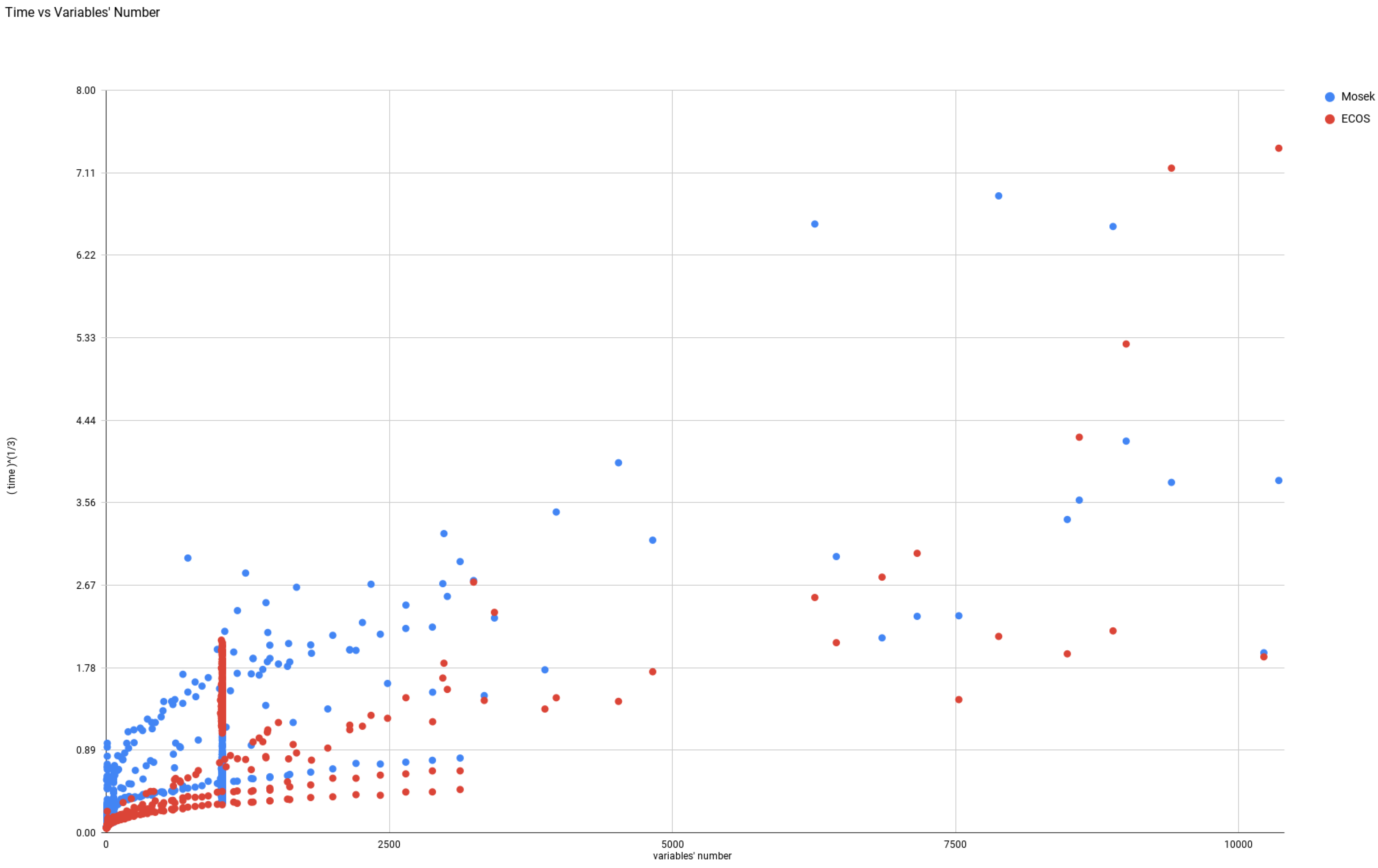
Two of the solvers, namely, Mosek and ECOS work very satisfactorily. Even though, ECOS sometimes was 1000 times faster than Mosek, on some of types 1 and 2 instances, the time difference was no more than 5 s making this advantage rather dispensable. Nevertheless, on these instances, Mosek had better optimality measures. Note that on the hard problems of type 1, namely, “RDNUNQXOR”, Mosek was faster than ECOS see Figure 1.

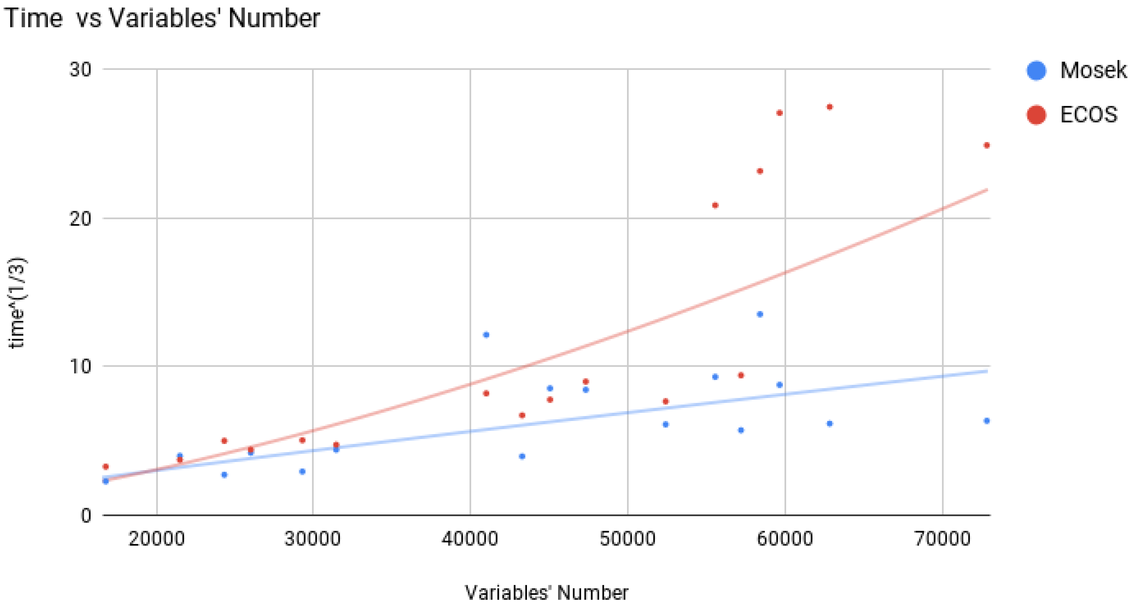
On the other hand, ECOS was slower than Mosek on the Gaussian instances especially when the (CP) had a huge number of variables. For these instances, the time difference is significant (hours) see Figure 2, which is rather problematic for ECOS.

Hence each of the two solvers has its pros and cones. This means that using both solvers is an optimal strategy when approaching the problem. One suggestion would be to use ECOS as a surrogate when Mosek fails to give a solution. Earlier ad-hoc approaches, which were based on CVXOPT and on attempts to “repair” a situation when the solver failed to converge, appear to be redundant.

References

- Bertschinger, N.; Rauh, J.; Olbrich, E.; Jost, J.; Ay, N. Quantifying unique information. Entropy 2014, 16, 2161–2183. [Google Scholar] [CrossRef]
- Williams, P.L.; Beer, R.D. Nonnegative decomposition of multivariate information. arXiv, 2010; arXiv:1004.2515. [Google Scholar]
- Griffith, V.; Koch, C. Quantifying synergistic mutual information. In Guided Self-Organization: Inception; Springer: New York, NY, USA, 2014; pp. 159–190. [Google Scholar]
- Harder, M.; Salge, C.; Polani, D. Bivariate measure of redundant information. Phys. Rev. E 2013, 87, 012130. [Google Scholar] [CrossRef] [PubMed]
- Bertschinger, N.; Rauh, J.; Olbrich, E.; Jost, J. Shared information—New insights and problems in decomposing information in complex systems. In Proceedings of the European Conference on Complex Systems, Brussels, Belgium, 2–7 September 2012; Springer: Cham, Switzerland, 2013; pp. 251–269. [Google Scholar]
- Nemirovski, A. Efficient Methods in Convex Programming. Available online: http://www2.isye.gatech.edu/~nemirovs/Lect_EMCO.pdf (accessed on 6 October 2017).
- Wibral, M.; Priesemann, V.; Kay, J.W.; Lizier, J.T.; Phillips, W.A. Partial information decomposition as a unified approach to the specification of neural goal functions. Brain Cognit. 2017, 112, 25–38. [Google Scholar] [CrossRef] [PubMed]
- Ruszczyński, A.P. Nonlinear Optimization; Princeton University Press: Princeton, NJ, USA, 2006; Volume 13. [Google Scholar]
- Bubeck, S.; Eldan, R. The entropic barrier: A simple and optimal universal self-concordant barrier. arXiv, 2014; arXiv:1412.1587. [Google Scholar]
- Bubeck, S.; Eldan, R. The entropic barrier: A simple and optimal universal self-concordant barrier. In Proceedings of the 28th Conference on Learning Theory, Paris, France, 3–6 July 2015. [Google Scholar]
- Boyd, S.; Vandenberghe, L. Convex Optimization; Cambridge University Press: Cambridge, UK, 2004. [Google Scholar]
- Makkeh, A. Applications of Optimization in Some Complex Systems. Ph.D. Thesis, University of Tartu, Tartu, Estonia, 2017. [Google Scholar]
- Nocedal, J.; Wright, S. Numerical Optimization; Springer: New York, NY, USA, 2006. [Google Scholar]
- Boyd, S.; Kim, S.J.; Vandenberghe, L.; Hassibi, A. A tutorial on geometric programming. Optim. Eng. 2007, 8, 67–127. [Google Scholar] [CrossRef]
- Chares, R. Cones and interior-point algorithms for structured convex optimization involving powers and exponentials. Doctoral dissertation, UCL-Université Catholique de Louvain, Louvain-la-Neuve, Belgium, 2009. [Google Scholar]
- Hahn, T. CUBA—A library for multidimensional numerical integration. Comput. Phys. Commun. 2005, 168, 78–95, [hep-ph/0404043]. [Google Scholar] [CrossRef]
- Lubin, M.; Dunning, I. Computing in operations research using Julia. INFORMS J. Comput. 2015, 27, 238–248. [Google Scholar] [CrossRef]
- Sra, S.; Nowozin, S.; Wright, S.J. Optimization for Machine Learning; MIT Press: Cambridge, MA, USA, 2012. [Google Scholar]
- Byrd, R.; Nocedal, J.; Waltz, R. KNITRO: An Integrated Package for Nonlinear Optimization. In Large-Scale Nonlinear Optimization; Springer: New York, NY, USA, 2006; pp. 35–59. [Google Scholar]
- Waltz, R.A.; Morales, J.L.; Nocedal, J.; Orban, D. An interior algorithm for nonlinear optimization that combines line search and trust region steps. Math. Program. 2006, 107, 391–408. [Google Scholar] [CrossRef]
- Byrd, R.H.; Hribar, M.E.; Nocedal, J. An interior point algorithm for large-scale nonlinear programming. SIAM J. Optim. 1999, 9, 877–900. [Google Scholar] [CrossRef]
- Byrd, R.H.; Gould, N.I.; Nocedal, J.; Waltz, R.A. An algorithm for nonlinear optimization using linear programming and equality constrained subproblems. Math. Program. 2004, 100, 27–48. [Google Scholar] [CrossRef]
- ApS, M. Introducing the MOSEK Optimization Suite 8.0.0.94. Available online: http://docs.mosek.com/8.0/pythonfusion/intro_info.html (accessed on 6 October 2017).
- Andersen, E.D.; Ye, Y. A computational study of the homogeneous algorithm for large-scale convex optimization. Comput. Optim. Appl. 1998, 10, 243–269. [Google Scholar] [CrossRef]
- Andersen, E.D.; Ye, Y. On a homogeneous algorithm for the monotone complementarity problem. Math. Program. 1999, 84, 375–399. [Google Scholar] [CrossRef]
- Domahidi, A.; Chu, E.; Boyd, S. ECOS: An SOCP solver for embedded systems. In Proceedings of the European Control Conference (ECC), Zurich, Switzerland, 17–19 July 2013; pp. 3071–3076. [Google Scholar]
- O’Donoghue, B.; Chu, E.; Parikh, N.; Boyd, S. Conic Optimization via Operator Splitting and Homogeneous Self-Dual Embedding. J. Optim. Theory Appl. 2016, 169, 1042–1068. [Google Scholar]
- O’Donoghue, B.; Chu, E.; Parikh, N.; Boyd, S. SCS: Splitting Conic Solver, Version 1.2.7. Available online: https://github.com/cvxgrp/scs (accessed on 6 October 2017).
- Grant, M.; Boyd, S. CVX: Matlab Software for Disciplined Convex Programming, Version 2.1. Available online: http://cvxr.com/cvx (accessed on 6 October 2017).
Figure 1.
Comparison Between the running times of Mosek and ECOS for problems whose number of variables is at below 10,500.
Figure 2.
Comparison Between the running times of Mosek and ECOS for problems whose number of variables is at least 16,000.
© 2017 by the authors. Licensee MDPI, Basel, Switzerland. This article is an open access article distributed under the terms and conditions of the Creative Commons Attribution (CC BY) license (http://creativecommons.org/licenses/by/4.0/).
Share and Cite
MDPI and ACS Style
Makkeh, A.; Theis, D.O.; Vicente, R. Bivariate Partial Information Decomposition: The Optimization Perspective. Entropy 2017, 19, 530. https://0-doi-org.brum.beds.ac.uk/10.3390/e19100530
AMA Style
Makkeh A, Theis DO, Vicente R. Bivariate Partial Information Decomposition: The Optimization Perspective. Entropy. 2017; 19(10):530. https://0-doi-org.brum.beds.ac.uk/10.3390/e19100530
Chicago/Turabian StyleMakkeh, Abdullah, Dirk Oliver Theis, and Raul Vicente. 2017. "Bivariate Partial Information Decomposition: The Optimization Perspective" Entropy 19, no. 10: 530. https://0-doi-org.brum.beds.ac.uk/10.3390/e19100530
Note that from the first issue of 2016, this journal uses article numbers instead of page numbers. See further details here.