Bayesian Inference of Ecological Interactions from Spatial Data


1
C3—Centro de Ciencias de la Complejidad and Instituto de Ciencias Nucleares, Universidad Nacional Autónoma de México, Circuito Exterior, A. Postal 70-543, Ciudad de México 04510, Mexico
2
Instituto de Biología, Universidad Nacional Autónoma de México, Circuito Exterior, A. Postal 70-543, Ciudad de México 04510, Mexico
3
Departamento de Ciencias Ambientales, CBS Universidad Autónoma Metropolitana, Unidad Lerma, Estado de México 52006, Mexico
*
Author to whom correspondence should be addressed.
†
These authors contributed equally to this work.
Entropy 2017, 19(12), 547; https://0-doi-org.brum.beds.ac.uk/10.3390/e19120547
Submission received: 4 September 2017
/
Revised: 6 October 2017
/
Accepted: 12 October 2017
/
Published: 25 November 2017
(This article belongs to the Special Issue Maximum Entropy and Bayesian Methods)
Abstract
:The characterization and quantification of ecological interactions and the construction of species’ distributions and their associated ecological niches are of fundamental theoretical and practical importance. In this paper, we discuss a Bayesian inference framework, which, using spatial data, offers a general formalism within which ecological interactions may be characterized and quantified. Interactions are identified through deviations of the spatial distribution of co-occurrences of spatial variables relative to a benchmark for the non-interacting system and based on a statistical ensemble of spatial cells. The formalism allows for the integration of both biotic and abiotic factors of arbitrary resolution. We concentrate on the conceptual and mathematical underpinnings of the formalism, showing how, using the naive Bayes approximation, it can be used to not only compare and contrast the relative contribution from each variable, but also to construct species’ distributions and ecological niches based on an arbitrary variable type. We also show how non-linear interactions between distinct niche variables can be identified and the degree of confounding between variables accounted for.
1. Introduction
At the heart of our scientific understanding of the world lies the notion that the world is composed of discrete objects—atoms, molecules, planets, genes, cells, individuals of a species, texts, etc.—and that there exist interactions between these objects. To describe, understand and predict phenomena, we need to be able to characterize both the nature of the objects and the interactions between them. Fundamental physics has been the most successful in this endeavor, where we have been able to deduce the existence of the fundamental building blocks of matter—electrons, quarks, etc.—and importantly, the four fundamental forces—gravity, electromagnetism, weak and strong nuclear forces—through which all interactions at any scale have their ultimate origin. Moreover, these forces only depend on a few simple characteristics of these building blocks: electric charge, color charge, weak charge and mass. Our qualitative and quantitative understanding of the building blocks of matter, and their interactions, is breathtaking, yielding a more precise agreement between theory (prediction) and experiment than any other area of science. Therefore, how did we arrive at such a high level of understanding? Essentially, all our knowledge was deduced from an analysis of data associated with the relative positions in space and time of objects, combined with the deduction of certain taxonomical information about those objects.
Unfortunately, once we go beyond fundamental physics, a quantitative description of the interactions, and the appropriate taxonomical labels with which to understand them, is much more difficult. How should they be identified and classified? How can we better understand interactions in other areas of science, such as genetics, or linguistics, or, as is of particular interest in this paper, ecology? Indeed, how should one characterize, or define, an interaction in the general area of Complex Adaptive Systems (CAS)? Our understanding of CAS is very much less than that of fundamental matter, due to the fact that, unlike physical matter, CAS are not classifiable in terms of a small number of fundamental properties, such as charge, mass, etc. Secondly, their interactions are not as universal. These characteristics are, in their turn, related to the extreme degree of multi-factoriality associated with CAS. This implies that to characterize them phenomenologically requires a huge amount of data. It is only recently, however, that such data have begun to be available due to the data revolution. The volumes associated with such data and their associated multi-factoriality also imply that new methodologies, such as machine learning and data mining, as opposed to traditional scientific computing, are required to model them.
In this paper, we will argue that, as with fundamental physics, a general framework for characterizing and quantifying interactions in a CAS is through analyzing the relative spatial positions, potentially in time, of the objects characteristic of the CAS under study, and using the statistical distribution of co-occurrences of the objects, relative to a null hypothesis associated with the non-interacting system, as a diagnostic for inferring interactions. In other words, if the distribution of co-occurrences is distinct from that of the non-interacting system, then we take that as an indication of the existence of an interaction. The question then becomes: what can be said about the specific properties of the interaction using that spatial data? By taking this pragmatic, empirical approach to defining an interaction, we avoid the pitfalls of trying to use subjective, expert, disciplinary knowledge to identify and categorize them. It may be thought that the requirement of datasets on the spatial distributions of each and every object is as severe a restriction as having detailed bespoke data about every potential interaction. However, this is not the case. Firstly, there are many more interactions than objects. Another important reason is that over the last couple of decades in particular, there has been a continuous and spectacular growth in the availability of spatial data. Through the use of location-aware devices for example, greater amounts of spatial data are being generated every day, ranging from scientific data, such as museum specimen collection data, or satellite weather services, to casual data from mobile applications. Furthermore, with the creation of open databases like the Global Biodiversity Information Facility (GBIF) (www.gbif.org) or governmental data services like www.data.gov, there are many data that are now publicly available. All these data contain implicit information about the interactions that shape our world and society. The challenge is to find better tools with which to transform that data into knowledge, in ways that are useful for a wider range of users, not only the professional analyst [1].
Although new techniques for analyzing spatial datasets have been developed in the last decade, most of them seem to be focused on analyzing small collections of large point sets and do not adjust well to analyzing large collections of point sets, where each point set corresponds to one variable and visual exploration is limited to a few characteristic features of the data [2]. As data mining is chiefly associated with seeking correlations or patterns in spaces with many variables, as opposed to a few, where a more classical statistical approach is appropriate, spatial data mining requires tools that are suitable for considering large numbers of spatial distributions considered as potential predictive variables. One technique for doing this is network graph analysis where we can use the network graph space to explore potential relationships.
Network graphs offer a rich structure that has been recognized in many fields as a helpful visual representation, due to their ability to represent complex systems of relationships in a visually insightful and intuitive way. Network graphs also provide a strong mathematical framework for algorithmic and statistical analysis, mainly from graph theory and, more recently, from complex systems. In particular, geographic information science has a long tradition in network analysis for the study of spatial networks [3]. Spatial networks are usually network graphs defined by a set of nodes representing spatial locations and a set of links representing some type of connection between locations. In these cases, network graphs are used as a third analysis space to explore the topological and geometrical properties of infrastructure networks [4], or to understand the dynamics of flows between spatial locations [5]. Although network graphs are consistently used in spatial networks, their use has not extended to spatial data mining in general when data are not already explicitly embedded in a network structure. In the ecological setting, Complex Inference Networks (CIN) [6,7] have been used to infer biotic interactions in an ecosystemic setting, particularly in the case of emerging diseases [8,9,10,11], though such networks will not be the focus of this paper.
Of course, there is a fundamental question as to whether a set of spatial data gives explicit information about an interaction versus information from which an interaction is to be inferred and potentially characterized. The vast majority of spatial data that are available has not been generated with the specific intention of analyzing a particular interaction. Rather, the data are used to infer the existence and nature of an interaction using a suitable mathematical framework for making statistical inferences. Bayesian inference [12] provides an appropriate framework for this task, where Bayes’ theorem is used to update the probability of a hypothesis, such as the existence and nature of an interaction, as more evidence or information becomes available. This is particularly appropriate in our cases of interest where we can deduce more information about the interaction by including more spatial information.
Although we will try to couch much of our discussion in general terms, considering three very different cases where interactions can be inferred and characterized using co-occurrence data and a corresponding statistical ensemble, our main concern is to apply these ideas to ecological interactions and, particularly, to the context of niche description. Of course, the use of co-occurrence data in ecology has a long history, with the particulars depending on whether we are talking about abiotic or biotic interactions. In the case of climatic data, species distribution modeling has used the co-occurrence between a point collection of a target species and the specific environmental conditions at that point, the latter being modeled as environmental layers at the pixel level [13,14]. Many different algorithms have been used to model the relation. Of special relevance given the topic of this paper is the maximum entropy algorithm [15,16], which has been extensively used. For biotic interactions, the inference of potential interactions from co-occurrence data goes back to [17], where it was used to look at species assemblages, with the co-occurrence data being associated with presence/absence of a species at a given site, originally an island. It was believed that the co-occurrence data could reflect inter-specific competition. Since then, the use of co-occurrence data, and the interpretation of the associated analysis to infer biotic interactions, has been controversial and, especially recently, has generated many papers; see, for instance, [18] for a recent discussion. We believe that much of the controversy is due to a lack of an empirical characterization of an interaction using the data under consideration; a phenomenological “definition” if you will. This is also linked to the question of whether an inferred interaction is “direct” or “indirect”.
This paper is based on a methodological framework [6,7,8,19,20] that has been developed to determine, characterize and quantify ecological interactions of any type, abiotic or biotic, using data of arbitrary spatial resolution. It allows one to characterize the full ecological niche of a taxon, while comparing and contrasting the contribution of each niche variable. The formalism has been applied successfully, chiefly in the area of zoonoses where it has led to the prediction and confirmation of many previously unknown vector-host interactions in several emerging or reemerging diseases [9,10,21]. In spite of its success in this important application area, it is not well known in a wider context, and importantly, its conceptual underpinnings and its general applicability to the general area of identifying and characterizing ecological interactions have not been exploited. As a complement to these papers, we will here concentrate on its conceptual and mathematical basis and, in particular, on how it can be used to deduce causal chains and identify confounding factors in any given ecological setting.
The format of the paper is as follows: In Section 2, we discuss how our knowledge of interactions has been gleaned from an examination of spatial data using an example from four very distinct areas: fundamental physics, population genetics, text mining and fundamental niche modeling. We note that the existence of interactions leaves an indelible imprint on the spatial distribution of the objects—atoms, genes, words, species, etc.—that are interacting and that, reversing the logic, the spatial distribution of objects may be used to infer the existence and nature of interactions. In Section 3, we discuss how direct versus indirect interactions have been characterized, emphasizing that the difference between one and the other is often a question of convenience and, importantly, of the spatial resolution at which we are examining the system. We note that the indirect nature of an interaction between two spatial variables is manifest when there are variables (confounding factors) that intermediate between them and that can be examined and seen to offer a more quantitatively precise description of the interactions. In Section 4, we show how to define co-occurrences to be used as diagnostics for the existence of interactions by comparing spatial distributions of co-occurrences relative to an expected benchmark associated with the absence of interactions. In Section 6, we quantify how the distribution of co-occurrences can be used to infer the existence of interactions and make a base characterization of them: attractive/repulsive, strong/weak. In Section 7, we show how the previous discussion applies concretely to the case of identifying and quantifying ecological interactions, and in Section 8, we illustrate the formalism with results from a concrete example: comparing and contrasting biotic and abiotic interactions in the distribution of the bobcat (Lynx rufus (Schreber 1777)). In Section 9, we discuss the wider implications of our formalism. Finally, in Section 11, we present the basic mathematical formalism that we use, which is a prerequisite for understanding the paper.
2. Characterizing Interactions Using Spatial Data
Before considering the characterization of interactions in ecology, it is worthwhile to consider how interactions have been identified and characterized using “spatial” data in other settings.
2.1. In Physical Systems
The area where interactions have been most successfully classified and quantified is in physics and, to a somewhat lesser extent, in chemistry. In the case of physics, the first interaction to be successfully studied was the gravitational interaction. Before a rigorous, theoretical understanding of gravity was obtained, it was well understood that celestial bodies were spatially discrete objects with a predictable dynamics. Much human activity depended on this predictability, but their taxonomy was founded on a terrestrial viewpoint, whereby planets, the Sun and the Moon were not differentiated in terms of understanding their role in the context of higher structures: planet/satellite and solar system. Based on the detailed and precise observations of Brahe, it was for Kepler to deduce from that data the “laws” that capture the phenomenological regularities associated with the movement of the planets. However, there was no notion of that movement being associated with the concept of an interaction between celestial bodies. It was for Newton to notice that if one object is in orbit around another, then it is in a state of acceleration and, therefore, according to his laws of motion, must be subject to a force, i.e., there must exist an interaction between the two bodies. Using Kepler’s laws and his own laws of motion, it was in fact possible to deduce the precise nature of this interaction, being associated with a postulated law of gravitation, wherein the force of interaction between two celestial bodies was proportional to the product of their masses and the inverse square of their distance. Moreover, given that mass is a positive number, it was possible to see that the interaction is such as to always give rise to an attractive force between bodies. The apocryphal tale of the falling apple is in the same vein, the falling to Earth of the apple being a consequence of the interaction between apple and Earth. Moreover, it was possible to postulate and verify that the nature of this interaction was truly universal in that it was associated with an interaction between any two objects with mass and depended on one, and only one, property of the associated objects: their mass. The crucial lesson from this is that it was possible to deduce the nature of the interaction between objects, both qualitatively and quantitatively, by simply observing the relative positions in space and time of these objects.
Without going into further detail, our understanding of the nature of the other types of interactions between physical objects has followed the same path. By observing the relative spatial positions of objects of distinct types, we have been able to deduce the existence of four fundamental interaction types: gravity, electromagnetism and the strong and weak nuclear forces; each possessing a high degree of universality, wherein the nature of the interaction depends only on a very small number of parameters: mass and different types of charge. In the case of some of the fundamental interactions, as in the case of electromagnetism, it is possible to also have repulsion, as well as attraction. By noting the relative spatial positions of electrically-charged bodies, it was possible to deduce analogs of Kepler’s and Newton’s laws, such as Coulomb’s law—the inverse square law for the force between charged bodies—which then were further subsumed into Maxwell’s equations, which fundamentally characterize the electromagnetic interaction.
Our ability to deduce the nature of the fundamental interactions very much depended on the existence of systems where the number of objects and the relationships between them were particularly simple. For instance, in the case of gravity, the fact that the mass of the Sun is so much larger than that of the planets led to a huge simplification in the dynamical analysis. Similarly, in the case of electromagnetism, the ability to arrange experiments where the charge of, and distance between, two objects could be precisely controlled facilitated greatly the deduction of the nature of the interaction.
Thus, we may state that experimental observation at different scales of the relative positions of physical objects and their subsequent spatial modeling has allowed us to completely characterize, both qualitatively and quantitatively, the nature of the interactions between objects in physics and to see that they can be grouped into just a very few fundamental categories, which are associated with a very small number of parameters, and to note where and when each one predominates. It is, in fact, the case that our success in modeling physical systems owes a very great deal to the fact that these fundamental interactions have quite different spatial regimes in which they predominate.
2.2. In Genetics
In standard population genetics, where genes are viewed as beads on a string, the concept of interaction is associated with the notion of epistasis [22]. In this setting, the degree to which two genes are linked, i.e., they co-occur, can be used as a measure of epistasis. If we consider the population frequency, , of an allele (blue/brown eyes, etc.) at a genetic locus i, where C can refer to whatever conditioning information we may consider pertinent for defining our population, we can also consider the joint distribution, for two alleles and , at two genetic loci i and j. The linkage disequilibrium coefficient [23] associated with and is defined as:
and is associated with the notion that and may be correlated, with the degree of correlation being measured by the deviation of their joint probability distribution from that of two independent distributions. This correlation may be positive or negative, depending on whether the alleles “co-occur” with more or less frequency than would be expected if they were independent, this independence being the null hypothesis with respect to which we will measure correlations. Although the correlation may have different origins, one especially important source is that of epistasis, arising from fitness/natural selection. In standard population genetics, the marginal fitnesses, , and , of the different genes can be incorporated, whereupon (1) becomes:
where is the average population fitness. This is the selection-weighted linkage disequilibrium coefficient [24]. Importantly, in the dynamical equations for the genotypes in the population, it is (2) that directly enters in the equations, not (1).
When , the genes are uncorrelated, and the system is said to be in linkage equilibrium. However, the effect of natural selection, as modeled by the fitness function, is to potentially move the system away from linkage equilibrium. If we assume that the fitnesses of the two genes are additive, i.e., , then starting off from linkage equilibrium, one can deduce that and prove that in the next generation, . The action of homologous recombination on the other hand is to diminish the linkage disequilibrium.
We will now put this example into language that is appropriate for the ecological setting: the genome/chromosome gives a spatial structure, wherein objects (genes) can be located. Thus, we may speak of the “co-occurrence” of two alleles on a genome/chromosome. A population of such structures offers a statistical ensemble within which we may ask how often do two alleles co-occur. is the frequency of such co-occurrence in this ensemble. Positive additive epistasis (the whole is greater than the sum of the parts) implies that the genes interact such that there is an added benefit to having the two alleles at the same time. Negative epistasis (the whole is less than the sum of the parts) is the contrary case. Epistasis leads to linkage (co-occurrence distinct from the null hypothesis of independent distributions). Thus, an observation of linkage in this setting is a necessary, but not necessarily sufficient, condition for the existence of an interaction.
It is important to understand that although the existence of linkage, i.e., co-occurrence beyond the independence hypothesis, implies the existence of an interaction, it does not determine the precise nature, neither at the microscopic (genotypic), nor the macroscopic (phenotypic) level, of that interaction. However, we may characterize phenomenologically the interaction by considering , where the sign of we can take as a measure of the sign of the interaction—positive/negative (“attractive/repulsive”)—and its magnitude as a measure of the strength of the interaction, as .
We also wish to note that interactions in genetics, as in physics and chemistry, may have differing degrees of directedness. For example, it may occur that two genes are linked, but this linkage is not direct, but through the intermediation of a third gene with which the two are directly linked. We are thus led to consider multiple genes.
2.3. In Text Mining
In text mining, as in genetics, there are the concepts of statistical ensemble and of co-occurrence. In this case, the ensemble is an ensemble of texts or documents, and the co-occurrence is in terms of a particular object in the text, usually words, though this is not obligatory. A co-occurrence, for, say, two words, is typically specified as having the two words appear in the same text/document or within a certain distance apart in the text/document as measured in the word sequence that forms the text. There are several measures that may be used to measure the degree of co-occurrence and to what degree the co-occurrence is statistically significant. A useful one, which is most in line with our other interaction measures, is the t score [25] defined as:
where C and X are two objects in the text. The t score is zero when there is no correlation between the textual elements C and X given a particular definition of co-occurrence. Clearly, t is analogous to the linkage disequilibrium , the only difference being the associated objects, genes versus words, and the definition of co-occurrence: same chromosome versus same text. As with genetics, we may define a notion of epistasis associated with the notion of linkage disequilibrium. In other words, two words, or other elements, are said to interact within a certain ensemble of texts if . Whether or not this interaction is statistically significant can be stated after specifying a certain confidence interval associated with the null hypothesis that the text elements are independent of one another.
2.4. In Ecological Niche Modeling
In ecological niche modeling [13,14], where predictive models are developed relating the geographic distribution of a species to abiotic factors, such as climate, the statistical ensemble is that of the set of pixels in the rasters that represent the climatic variable, such as average annual temperature. A co-occurrence in this case is the appearance of a geo-referenced point collection in a given pixel associated with a particular value of the climatic variable. Note that, in the case of a continuous variable, such as temperature, if measured to sufficient accuracy, then typically, there will be no more than one co-occurrence, as no two values of the temperature are likely to be precisely the same.
3. Direct versus Indirect Interactions
An important concept when discussing interactions is that of direct versus indirect interaction. This can be illustrated in the physical context by considering the difference between, say, a gas and a solid. For a gas of helium atoms, there are strong electromagnetic interactions between the nucleus of a given atom and its constituent electrons. The interactions between one helium atom and another are, however, negligible. Generally though, the interactions between atoms may be non-negligible, and that is what can give rise to molecules. Thus, the interaction between an electron and a proton in a hydrogen atom can be thought of as being “direct”, being describable directly in terms of the fundamental electrostatic attraction between the positively-charged proton and the negatively-charged electron. Two hydrogen atoms though may form a hydrogen molecule. In this case, the interaction between the atoms, although it has its origin in the electrostatic interaction, is not directly describable as a simple interaction between two point-like hydrogen atoms, but rather, between two objects that possess structure. The resultant effective interaction between the hydrogen atoms results in the formation of a covalent bond, where electron sharing leads to a stable balance of attractive and repulsive forces between the atoms. Importantly, the direct electrostatic interaction between two protons would be negative, leading to a repulsion between the protons. However, the effect of the intermediating electrons in the covalent bond is such as to lead to an effective attraction between the protons. Unlike the direct electrostatic interaction between the two protons, this interaction is “indirect” and is a consequence of the presence of other intermediating elements: the electrons. In a potential abusive use of ecological terminology, we could say that the repulsive “competitive” interaction between individuals of the proton species was turned into an attractive interaction by the “facilitation” of individuals of the electron species. The resulting indirect interaction between the protons, due to the presence of the electrons, we can then think of, and mathematically characterize, as an emergent, direct “effective” interaction. Going further, the well-known Lennard–Jones potential describing the short-range repulsion and long-range attraction between neutral atoms or molecules is an effective interaction that is more indirect than that of the covalent bond linking the constituent atoms of a given molecule. The important point is that labeling an interaction as direct or indirect is to some degree a question of convenience and a question of observational scale. An effective, phenomenological model of a chemical bond between atoms as a “direct” interaction may well be much more useful then trying to simultaneously model the multiple, underlying, more fundamental, direct interactions between the atomic constituents. However, if we examine the molecule exhibiting the chemical bond at higher energies, then these more fundamental interactions will become apparent. The important point to make is that how an interaction in a system is characterized in physics and chemistry, and the degree to which we describe it as direct or indirect, is very much a function of the scale at which we make observations of that system. Rather than having a rigorous differentiation between direct and indirect interactions, we should be better served to think of the degree of indirectedness of an interaction.
In contrast to physics, or even chemistry, in CAS, the qualitative and quantitative characterization of interactions is much more difficult. This is due to several factors. First of all, the number of labels, or properties, of the objects that characterize a CAS is much greater than in a physical system. Moreover, unlike in physics, we do not even know what is a complete list of relevant labels. For instance, a given organism can be simultaneously a prey, a predator, a mate, a parasite, etc. In physics, however, an electron has two labels: charge and mass. In both, each label is, in principle, associated with a distinct type of interaction: predation, reproduction, parasitism, etc. for the organism, and electromagnetism and gravity for the electron. In physics, there are only four fundamental interactions, although there are many more effective interactions that are useful for describing particular phenomena at a certain scale. However, there are not so many that they have not been almost wholly categorized and quantified. In contrast, in CAS, the number of interactions is much higher. Moreover, we do not have an adequate taxonomy for them. In fact, the number of potential interactions is so high that it is impossible in practice to imagine analyzing them with separate experiments. Additionally, the relevant degree of potential indirectedness in CAS is much higher than in physics. This can be perfectly illustrated in the context of a simple food chain, such as: carnivore → herbivore → plant → Sun. One would be tempted to argue that the interaction between carnivore and herbivore was more direct than between carnivore and plant. However, a perfectly acceptable predictive model for the carnivore distribution might be built using plants as niche variables. Moreover, the principle effect of climate on the carnivore distribution might well be an indirect interaction intermediated by the plant and herbivore distributions.
In our examples of CAS, genetics, text mining and ecological niche modeling, there also exists the concept of direct or indirect interactions, although their differentiation, as stated, is often more difficult than in physics. In genetics, a particular phenotypic trait may change significantly when an allele of a particular epistatic pair that are in linkage disequilibrium changes. However, this does not mean that one of those genes was directly, causally responsible for the phenotypic change. It may well be that there exists some other genetic element that intermediates the interaction between the two. Similarly, in texts, if we imagined a set of texts with a frequent appearance of the phrase “big, red bus” and calculated the co-occurrence (t-score) for “big ” and “red ”, one may well find a significant relation. However, the interaction between them would be indirect as it is mediated by the word “bus”. In the case of fundamental niche modeling, often it seems that the interaction between, say, temperature and the presence of a given species is “direct”. However, such an interpretation would neglect the high degree of indirectedness that may exist in ecological interactions. For instance, in a food chain, besides a potential direct effect, temperature may affect the distribution of a vagile carnivore much more through its impact on the distribution of the plant food sources of the herbivores that represent the chief prey species of the carnivore.
In summary, we may intuit the degree of indirectedness of an interaction between two objects/variables, A and B, by trying to determine if there exists one of more other variables, C, that are more directly linked to A or B. An ecological example would be where A is a carnivore with an important prey species C, and B is the principal plant food source of B. In this case, the interaction between A and B is intermediated by C. In the next sections, we will present a formalism, wherein this difference may be identified and quantified using co-occurrence data.
4. Co-Occurrence as an Indicator of Interactions
We have laid out the thesis that interactions between objects are a fundamental property of all systems, the main difference being the nature of the objects at a given scale and the precise qualitative and quantitative characterization of their interactions. We have also argued that our understanding of the nature of the interactions between objects is largely a result of observing their relative positions as a function of time. A fundamental characteristic of basically all known interactions is their locality. This locality can be observed of course. In physics, the “range” of an interaction can be precisely defined, once the interaction has been quantified. Thus, the very fact that the Moon orbits, i.e., is constantly closer to, the Earth rather than the Sun shows that the Moon’s motion depends more on its gravitational interaction with the Earth than with the Sun. Similarly, the fact that the Earth orbits, i.e., is constantly closer to, the Sun than to another star shows that the interaction between the Earth and the Sun is stronger than the Sun with another star. More basically, to a good approximation, the Moon interacts with the Earth, but not other elements of the solar system, while the Earth interacts with the Sun, but not with other stars. As another example, if we heat hydrogen gas, the hydrogen molecules will eventually dissociate into hydrogen atoms and, if we keep heating the gas to even higher temperatures, the atoms will ionize, and we will have a gas of free electrons and protons. The state of the system and the nature of the interactions can be deduced by observing the relative positions of the relevant constituents, quantum mechanical subtleties notwithstanding. Thus, the fact that in the case of hydrogen atoms versus hydrogen ions, the electrons are bound to the protons means that their positions are highly non-random, being correlated with the positions of the protons. In the same way for hydrogen molecules, hydrogen atoms are bound together so that their relative positions are highly non-random with hydrogen atoms in the same molecule being correlated, while those in distinct molecules are uncorrelated. Similarly, in genetics, two genes that are close together on a chromosome are typically more likely to show epistasis than two that are far apart. Furthermore, two words are more likely to be linked in a text if they are separated by few words as opposed to a great number of them.
As stated, the notion that physical interactions between objects can be inferred from their relative positions as a function of time has been fundamental. Compared to biology and ecology, however, the detailed nature of the interactions in physics are much simpler, much more universal and much more direct. In all cases, however, the nature of interaction is so as to affect the spatio-temporal distributions of objects. Thus, we would claim that a necessary condition for there to exist an interaction is that the spatio-temporal distributions of the corresponding objects—atoms, molecules, genes, words, planets, etc.—is altered, with positive “attractive” interactions causing objects to be closer together than they would otherwise be, while with negative “repulsive” interactions they tend to be further apart. A generic notion to characterize this difference between these different behaviors is that of co-occurrence, wherein we expect objects to co-occur more or less than expected according to the degree of interaction between them. This is certainly the case in physics, where the phenomenon of bound states—nuclei, atoms, molecules, …, planetary systems, galaxies, etc.—is ubiquitous. Thus, in almost any physical material, the vast majority of protons and neutrons are not randomly distributed in space and time, but are found only as constituents of nuclei. Similarly, the vast majority of electrons are not distributed randomly, but are found bound to nuclei to form atoms. Atoms in their turn are not randomly distributed in space and time, but are generally found bound to other atoms to form molecules or other structures, such as crystals. Protons and neutrons co-occur in nuclei more than electrons co-occur in atoms due to the fact that the interaction between nucleons is much stronger than the interaction between electrons and nucleus. Similarly, in genetics, nucleic acids are not randomly distributed, but are found bound together in the form of RNA or DNA molecules. In this case though, although there exist physical interactions, the fact that certain nucleic acids co-occur is partly due to natural selection. Lastly, the co-occurrences of a plant with an associated unique insect pollinator will be less random when compared to the distribution of the pollinator with an ecologically unrelated species, such as a large carnivore.
We will quantify this notion below. We can also turn this logic around and define any non-random degree of co-occurrence as being due to an “interaction”, knowing that a given set of co-occurrence observations may not be enough to fully understand or characterize the interaction. This will particularly be the case in ecology.
5. Quantifying Co-Occurrence
To quantify this notion, we must first address the question of how to define a co-occurrence. Here, for simplicity, we will restrict to co-occurrences in space rather than time, or space and time, though the formalism is readily extendable to both. If two variables/objects—genes, words, species—are to be considered as co-occurring, we need some notion of spatial resolution and, then, to determine what is the appropriate scale. To quantify spatial co-occurrence, we require a notion of locating objects in space and an associated distance measure for those objects.
We define a set, , of elementary spatial units, , such that and that these cells form a partition of a spatial region, . In genetics, these would be a set of elementary units, such as genes, into which the one-dimensional genome could be divided and which form a partition. In the case of ecology, as we will discuss below, they could be a set of two-dimensional squares that form a partition of a given spatial region. For two variables/observables/objects of types A and B, we consider the and representatives of the two types. For example, in genetics, these would represent the numbers of genes of the two types in , while in ecology, they might represent the numbers of point collections of the two species A and B in a given spatial region. A variable/observable/object of type A, , where x is a spatial point in and denotes the value of the variable A, located at x, is then defined to be present or not in the spatial cell , which we now denote with the index i, according to if or not, i.e., if the spatial point x lies in the i-th cell. Here, is the number of discrete categories into which the variable A has been divided. Thus, is a Boolean variable. We define a co-occurrence for two variables/objects and , located at the spatial points x and y, as an indicator function and , i.e., both objects are in the same spatial cell. The spatial cells then form a statistical ensemble where, in each cell, we may determine if there exists a co-occurrence. In the case of genetics, the ensemble is formed by one-dimensional genomes and, unless we decide to take into account the spatial position of these genomes as individuals in some external space, each member of the ensemble is unrelated to another spatially. However, we can identify positions x within a given genome, which has been partitioned into genes. Thus, x could be a position in the i-th gene, thought of as a spatial unit, such as a nucleotide within that gene. Therefore, the spatial ordering of genes on the genome can be used to identify a co-occurrence, but there is no higher order spatial relation between the co-occurrences as there is on a geographic space. In the same way, in text mining, the ensemble is the set of texts/documents, and a position x could be a letter position within a given document. As with genetics, the notion of co-occurrence is associated with a particular text/document, and there is no a priori higher order spatial relationship between documents.
In the case of ecology, the spatial cells have a relation one to the other, with forming a partition of a two-dimensional (this also generalizes to higher dimensional analogs) area. The cells themselves may be of different types, such as regular, fixed size squares or more irregular types such as census block groups used by the U.S. census. If we consider object types, A and B, such as species of atoms or biological species, then multiple co-occurrences are possible, depending on the spatial distribution of the objects. The number of co-occurrences is given by:
In this way, we count multiple variable/object pairs within the same spatial cell. We can also count by simply counting in each cell the occurrence of a given type, independently of how many examples of the type there are in the cell. In this case, the number of co-occurrences is given by:
where the indicator function is A and B are both present in the spatial cell i, and for simplicity, we have now and in the rest of the paper dropped the indices and . Given , we may determine the probability of a co-occurrence . We may also determine the conditional probabilities and . We may take and as measures of the degree of co-occurrence of the types A and B.
Cell Size
Having defined co-occurrences with respect to a spatial cell, we must also consider the problem of the dependence of the results on the cell size. In the case of spatial data mining, this problem was identified in 1934 [26], and it is known as the “Modifiable Areal Unit Problem” (MAUP) [27]. Although MAUP has been an active research area since the 1980s [28], it is still an open challenge to develop systematic methods to detect appropriate sampling scales [1] for spatial data. In the methodology presented here, MAUP is the consequence of the choice of grid resolution, which is allied with the question of optimally sampling events on that grid.
The general effect of cell size can be appreciated if we consider the limits of very large or very small cells. There are two general considerations: one is the effect of cell size on the effective size of the statistical sample to be analyzed, and the other is to do with its effect on the number of co-occurrences. For the former, as we are doing statistical analysis and hypothesis testing, it is natural to take advantage of the samples at our disposal as much as possible. If we have N events, then the maximum size of the sample of cells is also N. However, if the cell size is such that multiple, assuming they are independent, events occur in a given cell, then the effective sample size is reduced. For instance, for a random distribution of events, if the cell size is such that on average the number of events per cell is four, then a reduction in the cell size by a factor of two will probably lead to cells where the expected number of events per cell is closer to one. In other words, all else being equal, the number of cells should naturally scale as the number of events. For the case of co-occurrences, for a finite set of events, if we go to the limit of very small cells, it is clear that eventually, we will end up with zero co-occurrences. On the other hand, in the limit of very large cells, we will end up with only one co-occurrence as all the events will be in one cell.
A crucially important element also enters associated with the cardinality of the variables. For binary variables, such as presence/absence of a given species, a co-occurrence has only four possibilities for two species A and B: , , and . However, for the co-occurrence of presence/absence of a species and a continuous variable, such as average annual temperature, there is a very large number of possibilities, depending on the granularity of the temperature scale. For a temperature range with 400 gradations (–40.00 C), there are 800 possibilities denoting the presence/absence with temperature , presence/absence with temperature , etc. With such a fine-grained description, the number of co-occurrences will be severely restricted. It is thus important to also reach a degree of granularity that is appropriate for the sample sizes of the different variables.
Another added complication is that different objects or variables may have very different natural spatial scales, so that what would be considered a large/small cell size with respect to one variable might be small/large with respect to another. This depends on the system under consideration and, more universally, on the sample size of variables/objects within the statistical ensemble of spatial cells. Given the desire to determine the degree of co-occurrence with the greatest degree of statistical confidence and given spatial distributions of two variables/objects, A and B, with sample sizes and , we would like to maximize the number of co-occurrences, , between them. As the cell size diminishes, then , as two objects cannot occupy the same physical position, and, as it increases, , as every object will be in the same spatial cell. If our target variable of interest is A, thought of, for example as a species whose niche we wish to characterize, and we consider a third object C, then we will be concerned with co-occurrences of type and , with counts and , respectively, in order to understand how species B and C affect the distribution of A. If , however, then the natural cell size for co-occurrences of A and B will generally be very different to that for A and C. This would be the case, for instance, where B represents a set of geo-referenced point collections for a very rare species, and C represents the same for a very common species. In this case, choosing a spatial cell resolution that is optimal for C would lead to being very small. On the other hand, choosing a spatial cell resolution that is optimal for B could lead to many occurrences of C in one cell, and therefore, the number of co-occurrences is potentially less than it could be. This same problem arises in a particularly exacerbated form when C represents a climatic raster, such as average annual temperature. In this case, the natural scale for the variable is the pixel level. After a suitable coarse graining of the continuous temperature variable, into two categories for example so that the two variables under consideration have the same number of values, we can compare and , finding that , even though and may be similar. This will mean that the statistical significance of C will be much greater than that of B due to much larger sample sizes. Alternatively, if we make a predictive model at the scale of C, then the number of pixels where B contributes will be very small compared to that of C, hence its contribution to the overall predictions of a model that contains both will be minimal.
The choice of cell size has been investigated empirically [7], where it has been determined that an optimal resolution exists that maximizes the number of co-occurrences. This was done by considering how the number of co-occurrences, and of Section 11, varied as a function of the size of the spatial cells, of the degree of correlation between the considered distributions and the numbers and . It was found that there existed a maximum in the number of co-occurrences as a function of grid size, where the precise grid size at which the number was maximized depended on these parameters. It was also found that the sensibility of our methods to the spatial grid size in characterizing interactions is relatively small. This is due to the fact that when considering multiple distributions, although the precise values of, say, and could vary substantially as the cell size changed, their relative ranking, i.e., which one was bigger/smaller, was quite robust.
The notion of cell size may also arise in our genetic and text-mining examples. In both cases, we may apply limits to determine co-occurrence with respect to each ensemble element. Thus, in the case of chromosomes, we may restrict attention to co-occurrences within a certain genetic distance of each other. Similarly, in text mining, we may restrict co-occurrences to be associated with words that are within a certain distance of each other in the text.
6. Inferring Interactions
We have stated that interactions between objects, in all cases, affect the spatio-temporal distribution of those objects relative to what it would be in the absence of those interactions. Inverting the logic, we therefore posit that a difference in the spatio-temporal distribution of a set of objects, relative to some null hypothesis about the distribution in the absence of the interaction, is an indicator of the presence of an interaction. We take as our measure of the spatio-temporal distribution of objects the statistical distribution of their co-occurrences in space and time, defined with respect to some null hypothesis about the form of that distribution in the absence of interactions.
The most basic type of co-occurrence is that between two object types, A and B. We consider or , where is the number of co-occurrences of A and B over a statistical ensemble of N spatial cells. If this is larger/smaller than expected, we will use that to infer that there must exist an interaction, either direct or indirect, between A and B. However, in order to determine if, say, is large or small, we need to specify a baseline from which to measure it. There are several relatively equivalent baselines. For instance, we can quantify relative to , the probability to find the type A independently of the presence of B. Another benchmark would be to measure relative to . Both benchmarks contain the same conceptual starting point, that co-occurrence (correlation) is measured relative to a distribution where there is no correlation given that if . With this in mind, we may define several related interaction measures between A and B. First of all, we may take as a measure of interaction between the object types A and B, our linkage disequilibrium coefficient . If , then the types A and B co-occur more frequently than would be expected in the absence of interaction and less frequently than expected in the case . No interaction is defined as . We will take to infer that there is an “interaction” between the types A and B. Alternatively, we may define the quantities or , from Equation (13), to be measures of the degree of interaction between A and B. In the case of , the statistical significance of the interaction is given by as seen in Equation (6) below. We can compare and contrast and for different variables, determining which are attractive, which are repulsive, which are strong and which are weak.
In the case , or , we will say there is a positive, or attractive, interaction and in the case , or , a negative, or repulsive, interaction. To gain intuition for this, we can consider the case of celestial dynamics, where A represents the moons of the planets and B the planets themselves. Taking a uniform spatial grid with cells of size, say km, we would find that objects of type “moon” co-occur with objects of type “planet”, but that there are no planet-planet co-occurrences. This would lead to us to infer, correctly, that there are attractive interactions between moons and planets. The magnitude of will, in turn, inform us about the strength of the interaction. Generally speaking, the stronger the interaction, the greater the degree of correlation/co-occurrence.
If , and are determined from finite samples, then there is a possibility that the population estimates of , and have sampling errors, such that . In this case, the deduction and measurement of an interaction is a statistical inference where a statistical significance measure must be used to determine the degree of interaction. We will use the Bayesian inference framework discussed in Section 11. As we are considering objects as Boolean variables, a binomial test is appropriate, where the diagnostic is:
which measures the statistical dependence of A on B, relative to the null hypothesis that the distribution of A is independent of B, the no interaction benchmark. As the sampling distribution of the null hypothesis is a binomial distribution where, in this case, every cell is given a probability of having a point collection of A. The numerator of Equation (6), then, is the difference between the actual number of co-occurrences of A and B relative to the expected number if the distribution of point collections were obtained from a binomial with sampling probability . As we are talking about a stochastic sampling, the numerator must be measured in appropriate units. As the underlying null hypothesis is that of a binomial distribution, it is natural to measure the numerator in standard deviations of this distribution and that forms the denominator of Equation (6). In general, the null hypothesis will always be associated with a binomial distribution, as in each cell, we are carrying out a Bernoulli trial (coin flip). However, the sampling probability can certainly change. As discussed in Section 11, the quantitative values of can be interpreted in the standard sense of hypothesis testing by considering the associated p-value as the probability that is at least as large as the observed one and then comparing this p-value with a required significance level. Although it is that determines the degree of interaction, a diagnostic such as is necessary in order to quantify the degree of statistical significance of the observed interaction.
Of course, a caveat with the above p-value-oriented approach, as in any situation where many pairwise statistical comparisons are made, is that given a certain size ensemble a subset of correlations may be identified as significant and, therefore, as indicating the presence of an interaction, even though the correlation arises due to sampling effects. There are many ways to improve this situation by, for example, applying a Bonferroni correction or an ANOVA analysis.
Having discussed how to characterize an interaction between two objects/variables, we will now consider the joint impact of multiple variables, on one particular object type, C, as discussed in Section 11, concentrating on the posterior probability , which would represent the joint interaction between C and a joint set of variables . As Equation (6) will not help in this case, due to the fact that , we must resort to an approximation procedure in order to estimate it. As discussed in Section 11, a popular procedure is to use the maximum entropy principle to estimate it. An alternative is to use the naive Bayes approximation, seen in Equations (10) and (13).
Interpreting the effect of on C in terms of interactions, in this case, we see that the overall effect is additive in terms of the score functions, , and multiplicative in terms of the likelihoods . Thus, the overall interaction between C and is approximated as a set of linear interactions between C and each variable , such that any non-linear interactions between the are neglected. In this approximation, the interaction can be characterized by the sign of and its magnitude . In the absence of an interaction, , and so, implies that the variable is positively correlated with C, such that, when C occurs in a spatial cell, then co-occurs with a higher probability than in a cell where C does not occur, which we interpret, in analogy with the cases discussed above taken from physics and genetics, as an “attraction”. On the contrary, when , co-occurs with a lower probability than in a cell where C does not occur, which we interpret as a “repulsion”. The magnitude of this attraction/repulsion is given by . In this way, we may compare and contrast the signs and magnitudes of any set of variables of arbitrary spatial resolution determining which variables contribute positively/negatively to the spatial distribution of C and what is their relative importance.
Inferring Direct versus Indirect Interactions
Having defined the quantities , or , to be measures of the degree of interaction between a target object/variable C and the variable , we may compare and contrast and for different , determining which are attractive, which are repulsive, which are strong and which are weak. However, this does not tell us how direct the interaction is. How might one determine the degree of indirectedness of an interaction using co-occurrence data? First of all, how do we define such indirectedness? A natural way to define an interaction between objects/variables C and to be indirect is if there exists a variable such that , where the intuition is that generally a direct interaction should be stronger than an indirect one. This is certainly the case in physics where, for instance, atomic interactions are stronger than molecular interactions. If we wish to take into account sampling effects, then we will require that there does not exist any variable such that . Essentially, this condition is equivalent to the idea that there is no confounding variable that is more predictive for C than . Thus, to see if there are confounding variables, we must determine the degree to which there are non-linear interactions between the different , using, for example, as seen in Equation (16).
7. Inferring Ecological Interactions
7.1. Defining Ecological Interactions
In the previous sections, we have tried to be general in our discussion as to how to infer interactions from the spatial distribution of the objects that are interacting. We now wish to focus specifically on ecological interactions. In this case, the co-occurrences are between a given target taxon, C, and a set of niche variables, both abiotic and biotic, . Each variable, , is coarse grained into categories, . For species distributions, proxied by point collection data, a species is represented by a variable , or depending on the availability of absence data. Hence, . For an abiotic variable, such as average annual temperature, we divide the range into a number of, usually uniform, intervals.
We wish to construct the distribution , where we will interpret as determining the extent to which there is an interaction between the taxon C and the set of niche variables . corresponds to an effective interaction that is attractive, while , in contrast, corresponds to an effective interaction that is repulsive. Alternatively, we may use the score function , with denoting attraction, and denoting repulsion. In the language of ecological niches: the set of values where , , denotes conditions and, correspondingly, spatial cells that are particularly well/mal-adapted (niche/anti-niche) for the presence of C.
As emphasized throughout, we cannot calculate the distributions or directly and so must resort to an approximation. We will use the naive Bayes approximation, seen in Equations (10) and (13). The likelihoods and the score contributions can now be calculated directly, once we have specified a suitable ensemble of spatial cells. As mentioned, each variable may have its own characteristic sample size and, therefore, . We therefore define a spatial cell at a resolution appropriate for the full set of niche variables [6,7]. As each variable is discrete, we can define co-occurrences of any specific value of the niche variable with the target taxon C. Thus, in each cell, the variable value is “present” or not.
Having defined the quantities or to be measures of the degree of interaction between the target taxon C and the niche variable , where, in the case of , the statistical significance of the interaction is given by , we can compare and contrast and for different niche variables, determining which values or ranges are attractive, which are repulsive, which are strong and which are weak. Any spatial cell may be assigned a niche profile according to the values of the niche variables in that cell. The construction of then allows us to determine then to what extent the cell represents niche/anti-niche.
7.2. Interpretation Issues
There are many potential issues surrounding the identification of interactions from co-occurrence data, many of which have been discussed in the literature [18]. Much of this literature criticizes the notion of using co-occurrence data to infer ecological interactions, often citing counterexamples [29] where an apparent interaction, as inferred from such data, is not consistent with the “real”, known interactions in the system. Other papers [9], on the other hand, have shown that it is possible to infer biotic interactions in the context of vector-host interactions. We believe that much of the controversy lies in not characterizing in a more precise manner what is an interaction in the first place. Usually, what seems to be in mind when identifying an interaction is that it is, in some intuitive sense, a direct interaction, such as predation. As we have emphasized, however, in general, distinguishing between direct and indirect interactions is a convenience. More often than not, the relevant issue is to determine the degree of indirectedness of the interaction by determining if there are intermediating variables that better explain and predict. In ecology, the vast majority of interactions that determine the presence of a species will be indirect. In this vein, it is somewhat remarkable that fundamental niche modeling happily predicts species distributions based on climatic data without wondering to what extent there may exist biotic confounding factors, while at the same time, there can be skepticism about the identification of a biotic factor as originating an interaction with the supposition that there is a confounding abiotic variable.
8. Results
We will now consider some results from applying the mathematical framework of Section 11 to a concrete example. The example we will consider is the characterization of the ecological niche of the bobcat (Lynx rufus), a vagile carnivore with an ample range. All species collection data used are available from the Sistema Nacional de Información de la Biodiversidad del Consejo Nacional de la Biodiversidad (http://www.conabio.gob.mx/remib/doctos/snib.html). Climatic data are from www.worldclim.org.
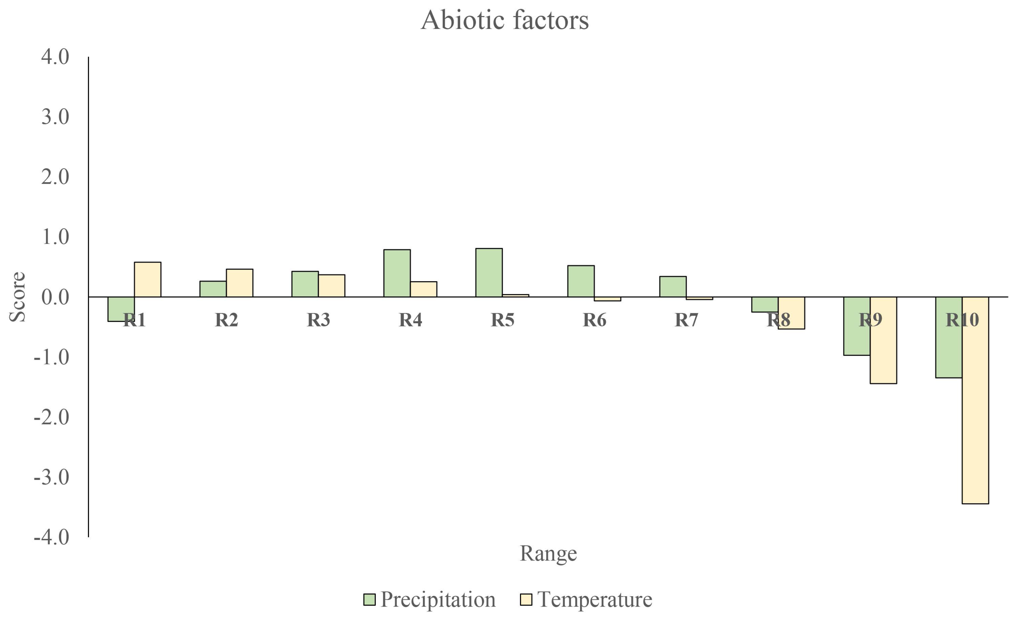
What can be gleaned first about the relative effects of biotic versus each range of values of abiotic factors in the niche of the bobcat? As a metric for the relative influence of biotic versus abiotic factors, we consider the score, , for both abiotic variables, particularly annual temperature and precipitation, which are the main resource used in fundamental niche modeling [13,14], and biotic variables, in this case, some of the actual or potential preys of the bobcat. Specifically, we consider the lagomorph group, which can represent up to 70% of the bobcat’s diet [30]. As mentioned, the interpretation of is that positive scores correspond to variables associated with the ecological niche, while negative scores correspond to an “anti-niche”.
In Figure 1 and Figure 2, we compare and contrast the relative contribution of each type of variable to the bobcat ecological niche. In Figure 1, we see the relative contribution of the abiotic variables where we have divided temperature (C) and precipitation (mm) into deciles with ranges: –15.2, –16.8, –17.9, –19.1, –20.4, –21.6, –23.1, –24.5, –25.7, –29.5) and –229, –315, –392, –482, –614, –767, –941, –1141, –1430, –4816), respectively (The ranges here are chosen to have roughly equal number of spatial cells in each one thereby giving each range the same statistical weight). The positive score of annual temperature and annual precipitation factors delineate the fundamental niche of the bobcat: precipitation values between 300 and 600 mm (prec R4 and R5) and temperatures from –20 C (–R3); whilst “anti-niche” conditions (i.e., negative score) correspond to low (<200 mm) and high (>1000 mm) precipitation values and temperatures >25 C. Turning now to the biotic niche variables, we note the lagomorphs Lepus californicus, Sylvilagus audubonii, Lepus callotis, Sylvilagus floridanus and Lepus alleni are all niche factors, while the lagomorphs Sylvilagus brasiliensis and Lepus flavigularis would fall into the anti-niche condition.
Note that in our methodological approach, we would describe the above results by saying that there is a weak positive/attractive interaction between the bobcat and temperature that decreases across ranges – and a negative/repulsive interaction that increase across the ranges – with the ranges and being associated with a strong negative interaction. For the biotic variables, we interpret the results by saying that Lepus californicus, Sylvilagus audubonii callotis, Sylvilagus floridanus and Lepus alleni are associated with a strong positive attractive/interaction with the bobcat, Sylvilagus cunicularius with a weak positive/attractive interaction, Sylvilagus brasiliensis with a weak negative/repulsive interaction and Lepus flavigularis with a strong negative/repulsive interaction. Note that the principal lagomorph scores are substantially higher than those of any abiotic range. However, no biotic factor is as negative as the highest temperature range. This seems to be a general characteristic found in other studies using our methodology [20], that biotic factors tend to dominate the most important positive/attractive interactions, while abiotic ones dominate the negative/repulsive ones. Of course, this does not imply that biotic interactions are always positive. Competitive exclusion, for example, will always be negative.
At this stage, we make no direct interpretation of the underlying nature of these ecological interactions. In particular, we make no assumptions as to how direct/indirect they are. We can, however, begin to establish hypotheses in this regard if we use knowledge of properties of the species under study, but without assuming anything about the potential interaction between them. With the knowledge that the bobcat is a vagile carnivore and the lagomorphs under consideration are herbivores of a substantially smaller size than the bobcat, we may make the hypothesis that the lagomorphs are prey species of the bobcat. This would be positing a direct interaction-predation. Further, we may posit that Lepus californicus is a more important prey species than Sylvilagus cunicularius. In our study case, we conducted a survey of food habits of Lynx rufus, finding that the high scoring species Lepus californicus, Sylvilagus audubonii and Sylvilagus floridanus represent the main diet items of the bobcat [31,32,33]. Thus, our hypothesis is consistent with this information. We may wonder, however, why, for example, there is an effective repulsion between the bobcat and Sylvilagus brasiliensis as, at first glance, it appears to fulfill the requirements of being a potential prey.
With the abiotic factors, there is a clear profile in both temperature and precipitation, with positive scores that generally speaking are lower than our chosen biotic factors. However, notably, the effect of high temperature or high precipitation, and especially the former, is associated with a particularly strong repulsion. May this repulsion be a “direct” effect? If so, how would we interpret such a direct effect? That the bobcat overheats easily; or may it be that it is an indirect effect intermediated by a complex food chain for instance?
An important advantage of our modeling framework is that it allows us to establish a transparent and unique ecological profile for any species using any niche variable that may be described in terms of a spatial distribution, thereby allowing us to quantify the relative influence of each niche variable, both biotic and abiotic, at each geographic location and its impact on the presence of a species there.
We have argued for a pragmatic approach to the identification and characterization of ecological interactions using spatial data. However, a criticism of this type of approach has been the potential presence of confounding factors. This is, of course, a problem in the analysis of any CAS where causal chains of events are very complex and it is difficult to separate causation from correlation. A typical arguments runs thus: we cannot know that there is a “direct” interaction between the bobcat and a lagomorph simply by looking at their co-association. It may be that the high score of Lepus californicus is confounded by the fact that it and the bobcat share the same climatic niche. In our interpretation, we are characterizing the co-occurrence of the bobcat and Lepus californicus as an interaction without going out on a limb to say it is definitely as a result of the predator-prey relationship. We infer the interaction and claim that the predator-prey hypothesis is consistent with what is known about the two species. However, we may go further and try to test to what extent abiotic factors may confound this interpretation. First up is the fact that, Lepus californicus, for example, has a much higher score than any abiotic variable. If annual temperature or annual precipitation were confounders, one would expect their score with bobcat, and Lepus californicus, to be higher than the score of bobcat with Lepus californicus.
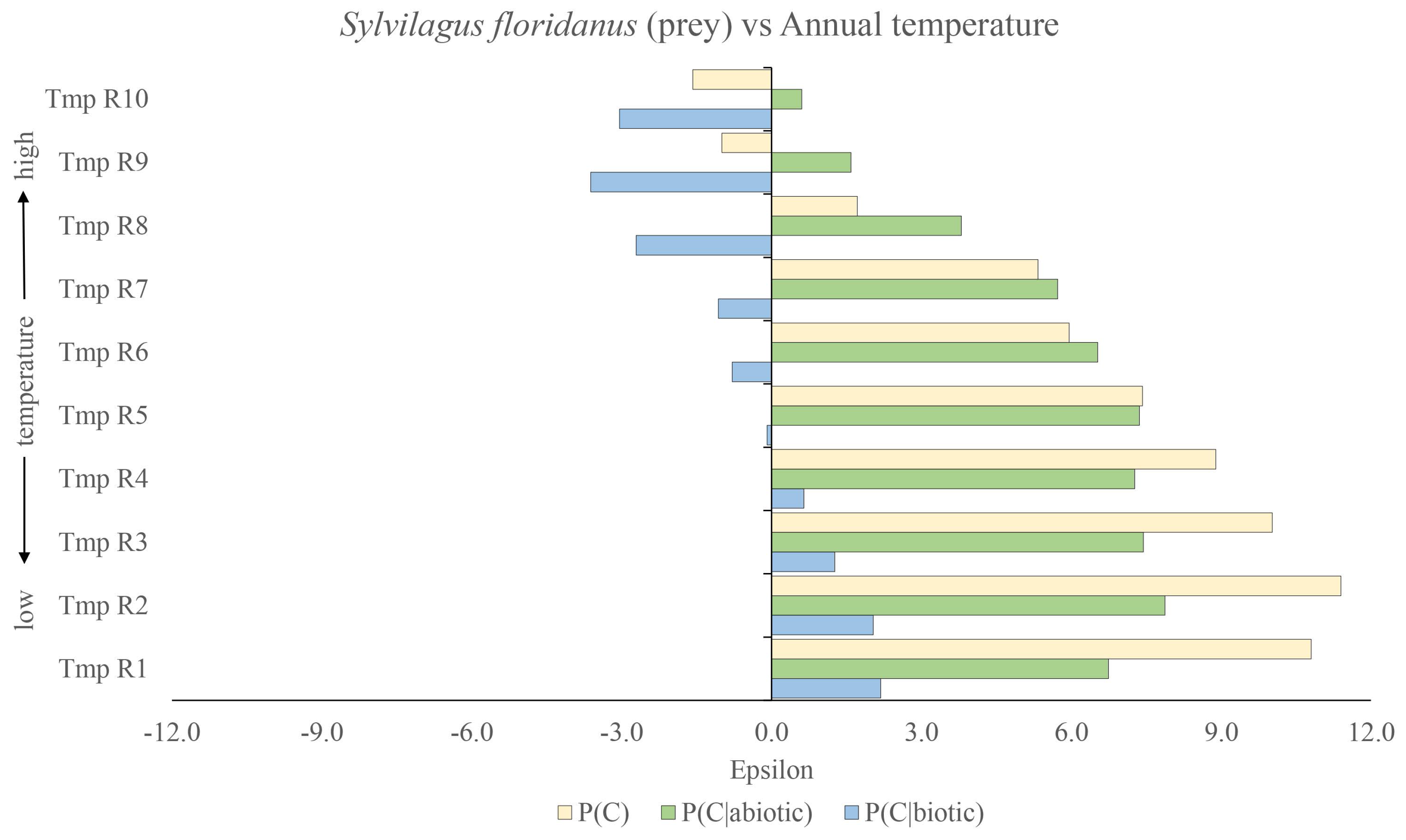
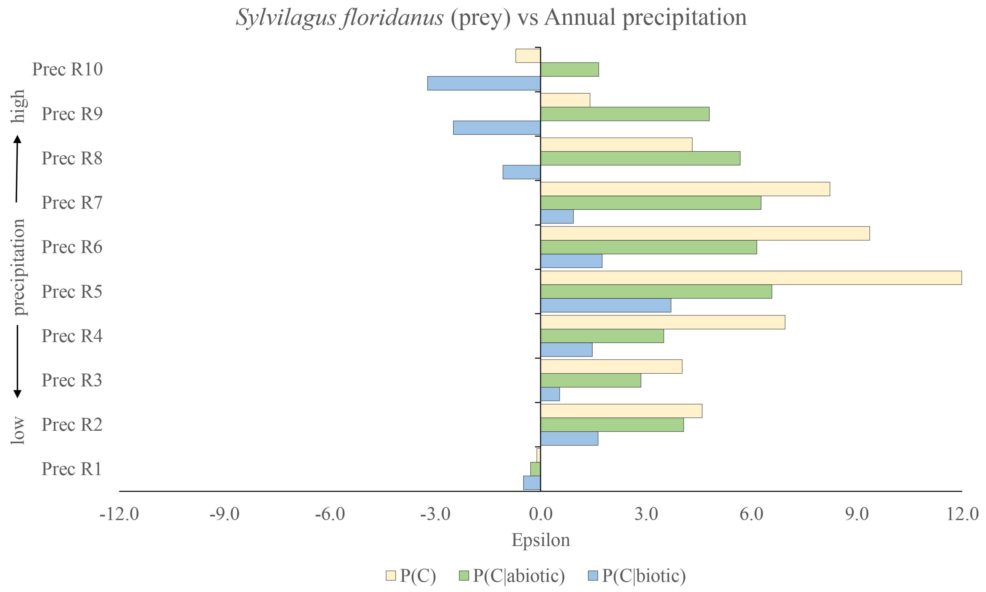
We can, in fact, quantify this even more by turning now to the relative effects of the various factors, considering the impact of the presence of the prey species Sylvilagus floridanus (biotic factor) relative to the contribution from the two climatic variables: annual temperature and annual precipitation (abiotic factors). We use Equations (18)–(20), where the three corresponding null hypotheses are , and . The results can be see in Figure 3 for annual temperature and in Figure 4 for annual precipitation. In Figure 3, the blue lines are associated with using as the null hypothesis, while the green lines are associated with using as the null hypothesis and the cream lines with as the null hypothesis. With respect to the latter null hypothesis, we can see that the optimal niche conditions for Lynx rufus are Sylvilagus floridanus present and temperature range . We can see that temperature range is slightly sub-optimal, as is range and successively, passing to higher and higher temperatures, yielding more and more sub-optimal conditions. Given that in Figure 1, we saw that temperature range was optimal, we may note that, as we are only considering the presence of Sylvilagus floridanus, there is a degree of non-linearity in the joint influence of annual temperature and presence of Sylvilagus floridanus on the presence of the bobcat. This non-linearity is even more pronounced in the case of presence of Sylvilagus floridanus and the effect of precipitation. Using our metric from Equation (17), for instance, we can determine that Annual precipitation = R7) = 3.54, i.e., that the correlations between these two niche variables for predicting the presence of the bobcat are statistically significant, thereby indicating a strong non-linearity in the joint influence of annual precipitation in this range and presence of Sylvilagus floridanus on the presence of the bobcat. This is also manifest in the fact that, while and , Annual precipitation = R7) = 0.36.
Additionally, the fact that the magnitude of the green lines is much greater than that of the blue lines clearly shows that the biotic factor—presence of the prey species Sylvilagus floridanus—is much more significant than the abiotic factor and that therefore the latter can in no way be a confounding factor responsible for the strong positive score of Sylvilagus floridanus. Furthermore, we may here see the joint impact of two niche variables together noting, for instance, that in spite of the presence of the prey species Sylvilagus floridanus, for temperature ranges and , the repulsive effect of the abiotic factor dominates and the overall combination is anti-niche. However, the combination , would be even more anti-niche.
We can see the same pattern depicted in Figure 4 for the case of precipitation. Once again, we can see the relative importance of the biotic factor being greater than that of the abiotic one. Of course, one could argue that there exist other potential abiotic confounders that we are not accounting for here. In any CAS, there is indeed a possibility that there exist confounders that are not explicit in the data being considered.
9. Discussion
Identifying, characterizing and quantifying ecological interactions is clearly a very important problem, both theoretically and practically. Physical interactions, we have seen, can be categorized at a given scale by the concept of an “effective” interaction, such as in the case of inter-molecular interactions, which are only related indirectly to underlying, more fundamental electromagnetic interactions. Thus, direct interactions, associated with more fundamental degrees of freedom at one scale, can give rise to indirect ones at another; so too in ecology. There, we can sensibly take fundamental interactions to be between individuals: the analogs of the electromagnetic, gravitational, weak and strong forces. At the level of interactions between individuals, a parasite must be located with its host, a predator with its prey, a pollinated plant with its pollinator, etc. Each interaction is local in space and time. The question is: what imprint is left from such individual interactions at larger scales, both in space and time? Can “micro”-interactions be discerned and quantified by more macro-level data?
As we have argued that, in other areas, micro-interactions have been discovered and analyzed precisely from more macro-phenomena, so too we propose that a consistent, empirically based way to characterize ecological interactions at the macro level, analogous to what is done in many other scientific areas, both in the past and now, is through the statistical distribution of co-occurrences of taxa, both between themselves and with any other spatial variable. The statistical distribution of these co-occurrences is defined via a statistical ensemble of units within which the specific co-occurrences of any set of spatial variables can be measured irrespective of the natural spatial resolution of the variable. The presence of an interaction is then defined by deviations of this statistical distribution with respect to some benchmark associated with the non-interacting system. Intrinsically, we have a probabilistic notion of interaction, where we determine that the probability, , of observing the event C is enhanced by the presence of . We may of course ask if there is any causality to this relation, rather than just correlation. Thus, we may ask to what extent any is a necessary or sufficient cause for C to be present?
Such notions certainly impact on our interpretation of , but not on its quantification. In practical terms, we may determine if is positive or negative and, importantly, if it is statistically significant with respect to our ensemble. A positive correlation we interpret as an “attractive” interaction, in that C and are more likely to co-occur than would be expected, and a negative correlation as a “repulsive” interaction, in that C and are less likely to co-occur than would be expected. There are, of course, many underlying reasons why two species may be “attracted”—parasitism, mutualism, facilitation, predation, etc., with probabilities that would not necessarily be expected to be symmetric. We can also determine the strength of the interaction through our score function . A strong interaction in this sense signifies a niche variable that discriminates spatially very well between those spatial regions where C is present versus those where it is not.
Therefore, how do we go beyond characterizing an interaction as attractive/repulsive or weak/strong? To do so, we need more information about the objects that are interacting. Taking our example from Section 8, we determined the presence of a strong attractive interaction between two species: Lynx rufus and Lepus californicus. What more can be said? If we add in the information that Lynx rufus is a mid-size, vagile, feline predator and that Lepus californicus is a herbivore about 10% of the size of the bobcat then a logical hypothesis would be that their strong degree of co-occurrence is due to the fact that Lepus californicus is a significant prey species of the bobcat. To verify this hypothesis, we may appeal to other previous research, or if this is not available, verify or falsify it directly through field work. This might seem like a trivial example, but precisely this logic and process have been used to predict and then confirm previously unknown hosts of emerging or neglected diseases, such as Leishmaniasis [9,34].
Of course, not all interactions identified from co-occurrence distributions will have such a simple interpretation. For instance, in the case of the repulsive interaction between the bobcat and Sylvilagus brasiliensis, we may hypothesize that there is a competitive interaction between them. Naturally, taking into account their aforementioned characteristics, we would be skeptical of such a relation. Without a natural explanation of a direct interaction, we would therefore be encouraged to look for potential confounding factors. Indeed, we saw that the abiotic factors annual temperature and annual precipitation could, indeed, act as confounders, giving rise to such a repulsive, indirect interaction. In any given situation, there is no set answer as to whether biotic versus abiotic effects are more likely to be confounders. However, our formalism is capable of deducing to what degree a given variable is confounded by another. In so doing, it detects the degree of non-linearity between different niche variables.
10. Conclusions
We have here proposed that a characterization and quantification of ecological interactions can be achieved, in analogy with other scientific areas, by an analysis of the relative positions in time of different ecological units. Of particular interest is the calculation of the niche of a species, represented by , the probability to find the taxon C given the full set of abiotic and biotic niche factors . This cannot be computed directly. However, by adopting an approximation scheme, such as the naive Bayes approximation, the entire niche, and anti-niche, of any taxon C can be characterized through this function, where any and every potential niche variable, , of any spatial resolution or type may be included and compared and contrasted with any other niche variable. We believe our Bayesian inference framework based on a statistical ensemble where all spatial variables are brought to the same spatial resolution is robust, predictive and can be applied to a large number of ecological problems. The chief data sources for biotic variables are large public databases, such as GBIF. Of course, such datasets have their own challenges in terms of data quality and data bias. Another challenge is to incorporate in such databases extensive metadata, beyond pure taxonomic classification, as this can be very important in permitting us to refine our hypotheses about the nature of any identified interaction. Indeed, generally speaking, the more distinct types of data variable, and their time dependence, we can input, such as species dispersal ability, deforestation, land use, socio-economic data, etc., the richer the set of variables we have for characterizing the niche of a taxon both spatially and, potentially, temporally.
11. Materials and Methods
We consider the joint probability distribution for a target class, C, and a set of predictive features . In the ecological setting, if C is a target taxon, would be considered to be the set of potential abiotic and biotic ecological niche dimensions, such as temperature, precipitation, presence/absence of other species, etc. Using Bayes theorem, we may write as:
and consider the posterior conditional probability distribution where:
which demonstrates how to update the prior probability distribution in the light of the information via the likelihood and the evidence . The overall goal is to estimate, from data, or .
In high dimensional situations, where there are more feature value combinations than data points, then neither nor may be calculated directly from a statistical ensemble as , i.e., every element is absent or unique. In this case, an approximation method must be found with which to model given a certain set of data. A standard estimation procedure is to use the maximum entropy principle [35,36] wherein:
where is a normalization constant, and the are parameters to be optimized, given the feature functions , in order to maximize the likelihood of given the data. Note that the feature functions are not constrained to be the same as the features themselves but could be functions of them. Here, M is the number of feature functions that will be used as constraints in the determination of the maximum entropy probability distribution.
An alternative and popular approach is to assume independence of the features in the likelihood and write:
This is the well-known naive Bayes approximation that is still extensively used in many situations [37,38,39,40,41,42,43,44,45]. The maximum entropy algorithm and the naive Bayes approximation are closely related [46], as the latter can be written in maximum entropy form, but with a Gibbs distribution that is factorizable. Each method for constructing has its advantages and disadvantages. The chief criticism of the naive Bayes approximation is its strong assumption of feature independence. In spite of this, it works, almost unreasonably, well. As has been pointed out and quantified [47], one reason the naive Bayes approximation works better than expected is that the correlations between features, which can be quantified via the coefficients (1) seen in Section 2.2, can be both positive or negative across different feature combinations. Moreover, due to the conservation of probability, we have:
which implies that, for any given pair of features, at least one correlation must have a different sign to the rest and, therefore, there must be cancellations for every pair of features. The maximum entropy model in contrast makes no such assumption. However, it is much more computationally expensive than the naive Bayes approximation. It is also quite sensitive to the specific choice of features that will be used to optimize on. The independence assumption can also be improved upon in the case of the naive Bayes approximation; for instance, by seeking those feature combinations that exhibit significant correlation and treating them together [47]. This can be done, once again, using the coefficients defined in Equation (1) in Section 2.2, so that if , where M is some appropriately chosen bound, then the features and should be considered together. For instance, for three features , and , the likelihood, , in the naive Bayes approximation is . However, if we determine that there is significant correlation between, say, and , we may write alternatively . It is then a question of determining which factorization offers a better fit to the data.
Given that the evidence function is not relevant for classification often, instead of the posterior probability directly, a score function:
is used, where is the complement of C. Using the naive Bayes approximation for both and , we have:
where is the score contribution from the feature . A feature with contributes positively to the posterior probability of a given instance being in the class C and, on the contrary, for .
Independent of the method used, an important task is to compare and contrast the contributions of the different features, and/or feature combinations, to obtain a better understanding of their relative importance. For individual features, , an appropriate measure of their relative importance and associated statistical significance is via a binomial test. This may be implemented at the level of the joint probability distribution :
or at the level of the posterior probability :
where the relative importance of is gauged relative to the null hypothesis that the distribution of C is independent of . In the case where the binomial distribution may be approximated by a normal distribution, then corresponds to the confidence interval for consistency with the null hypothesis. Of course, when there are sufficiently many , then some will be statistically significant for any chosen p-value. This is nothing new, and there are many methods that may be used to ameliorate this effect, a principle one being to have some intuitive notion of why it should be significant in the first place. Note that unlike , , i.e., it is asymmetric in its arguments, thus modeling the fact that the effect of on C may not be the same as that of C on .
The impact of correlations/epistasis/interactions between features on the calculation of can be quantified using the notion of linkage. The function gives a measure of the deviation of the joint distribution from a product form, which we will take to be a measure of the degree of interaction between C and . As , we see that (15) is also a measure of the degree of interaction between the variables, with the latter also providing confidence intervals for that interaction given a finite sample size. When determining the impact of a pair of features, and , we may follow the same procedure as for one variable, considering the joint probability distribution . In this case [47]:
Significant deviations from the null hypothesis indicate the presence of significant correlations, which we interpret as interactions. In this case, the interaction is ternary from the point of view of and and C, though one can also consider it to be binary if we consider as a combination. In analogy with , we can use a binomial test to determine the degree of consistency with the null hypothesis considering [47]:
Equation (17) determines when there is statistically significant interaction between the features and . Instead of considering the likelihoods, we may also consider the posterior probability directly. To determine the impact of a pair of features, and , we may follow the same procedure as for one variable, considering:
Once again, in the case where the binomial distribution may be approximated by a normal distribution, then corresponds to the confidence interval for the consistency with the null hypothesis. In this case, however, (18) cannot distinguish between the relative contributions of versus . This can be done, however, by considering alternative null hypotheses. Considering as null hypothesis , we have:
and similarly,
Equations (19) and (20) can be used as measures of the relative impact of one variable versus another. For instance, (19) expresses the contribution of the variable to the posterior probability , i.e., in the presence of the feature , but relative to the contribution marginalized over . These equations, in principle, allow us to determine which, of a combination of two variables, is the most important in terms of prediction of the class variable. Moreover, they facilitate the determination and analysis of confounding variables. As an example, imagine we determine that is significant, but hypothesize that there exists a confounding variable . In this case, we may consider and . If is, indeed, a confounding variable, then we should find that as the real influence on C is from , and so, if we take as null hypothesis, we should find little residual predictability.
Note that (17) can be used [47] to identify those feature combinations that should be considered together, and this information used to generate a generalized Bayes approximation [47], where the factorization of the likelihoods is not maximal.
In applying the above formalism, we define first a statistical ensemble of elements—genomes/ chromosomes, texts, two-dimensional spatial grid cells, three-dimensional spatial cubes, etc.—and the notion of a co-occurrence of objects within these elements. In genetics, the co-occurrence may be two genes in the same chromosome, the chromosome being an element in the ensemble. In text mining, the co-occurrence is, for example, two words within a certain distance of each other in the same document, where each document is an element in the ensemble. For molecules, a co-occurrence could be finding the atoms that potentially constitute the molecule in the same three-dimensional spatial cell and at the same time, each cell being an ensemble element. In ecology, a co-occurrence is two collection points within the same two-dimensional grid cell with, again, a spatial cell being an ensemble element.
Thus, in any of these examples, we calculate from , where is the number of co-occurrences of C and in the ensemble and is the number of occurrences of in the ensemble. As emphasized, calculating directly in the case where is of high dimension is not feasible as, typically, there will be only one or zero co-occurrences of the variables and in the ensemble. It is for this reason that approximation procedures, such as maximum entropy or naive Bayes, must be used.
Acknowledgments
We are grateful for financial support from DGAPA-PAPIIT grant IG200217.
Author Contributions
C.R.S. conceived the original ideas; C.R.S., C.G.S. and V.S.C. developed and applied the formalism; C.R.S. and C.G.S. analyzed the data; C.R.S., C.G.S. and V.S.C. wrote the paper.
Conflicts of Interest
The authors declare no conflict of interest.
Abbreviations
The following abbreviations are used in this manuscript:
| CAS | Complex Adaptive System |
| MAUP | Modifiable Areal Unit Problem |
References
- Andrienko, G.; Andrienko, N.; Demsar, U.; Dransch, D.; Dykes, J.; Irina Fabrikant, S.; Jern, M.; Kraak, M.-J.; Schumann, H.; Tominski, C. Space, time and visual analytics. Int. J. Geogr. Inf. Sci. 2010, 24, 1577–1600. [Google Scholar] [CrossRef]
- Guo, D. Flow mapping and multivariate visualization of large spatial interaction data. IEEE Trans. Vis. Comput. Graph. 2009, 15, 1041–1048. [Google Scholar] [PubMed]
- Curtin, K.M. Network analysis in geographic information science: Review, assessment, and projections. Cartogr. Geogr. Inf. Sci. 2007, 34, 103–111. [Google Scholar] [CrossRef]
- Xie, F.; Levinson, D. Measuring the structure of road networks. Geogr. Anal. 2007, 39, 336–356. [Google Scholar] [CrossRef]
- Rae, A. From spatial interaction data to spatial interaction information? Geovisualisation and spatial structures of migration from the 2001 UK census. Comput. Environ. Urban Syst. 2009, 33, 161–178. [Google Scholar] [CrossRef]
- Stephens, C.R.; Heau, J.G.; González, C.; Ibarra-Cerdena, C.N.; Sánchez-Cordero, V.; González-Salazar, C. Using biotic interaction networks for prediction in biodiversity and emerging diseases. PLoS ONE 2009, 4, e5725. [Google Scholar] [CrossRef] [PubMed]
- Sierra, R.; Stephens, C.R. Exploratory analysis of the interrelations between co-located boolean spatial features using network graphs. Int. J. Geogr. Inf. Sci. 2012, 26, 444–468. [Google Scholar] [CrossRef]
- González-Salazar, C.; Stephens, C.R. Constructing ecological networks: A tool to infer risk of transmission and dispersal of leishmaniasis. Zoonoses Public Health 2012, 59, 179–193. [Google Scholar] [CrossRef] [PubMed]
- Stephens, C.R.; González-Salazar, C.; Sánchez-Cordero, V.; Becker, I.; Rebollar-Tellez, E.; Rodríguez-Moreno, A.; Berzunza-Cruz, M.; Balcells, C.D.; Gutiérrez-Granados, G.; Hidalgo-Mihart, M. Can you judge a disease host by the company it keeps? Predicting disease hosts and their relative importance: A case study for Leishmaniasis. PLoS Negl. Trop. Dis. 2016, 10, e0005004. [Google Scholar]
- Rengifo-Correa, L.; Stephens, C.R.; Morrone, J.J.; Téllez-Rendon, J.L.; González-Salazar, C. Understanding transmissibility patterns of Chagas disease through complex vector-host networks. Parasitology 2017, 144, 760–772. [Google Scholar] [CrossRef] [PubMed]
- Ibarra-Cerdeña, C.N.; Valiente-Banuet, L.; Sánchez-Cordero, V.; Stephens, C.R.; Ramsey, J.M. Trypanosoma cruzi reservoir-triatomine vector co-occurrence networks reveal meta-community effects by synanthropic mammals on geographic dispersal. PeerJ 2017, 5, e3152. [Google Scholar] [CrossRef] [PubMed]
- Berger, J.O. Statistical Decision Theory and Bayesian Analysis; Springer: Berlin, Germany, 1985. [Google Scholar]
- Elith, J.; Leathwick, J.R. Species distribution models: Ecological explanation and prediction across space and time. Annu. Rev. Ecol. Evol. Syst. 2009, 40, 677–697. [Google Scholar] [CrossRef]
- Townsend Peterson, A.; Soberón, J.; Pearson, R.G.; Anderson, R.P.; Martínez-Meyer, E.; Nakamura, M.; Araújo, M.B. Ecological Niches and Geographic Distributions; Princeton University Press: Princeton, NJ, USA, 2011. [Google Scholar]
- Phillips, S.J.; Dudík, M.; Schapire, R.E. A maximum entropy approach to species distribution modeling. In Proceedings of the Twenty-First International Conference on Machine Learning, Banff, AB, Canada, 4–8 July 2004; pp. 655–662. [Google Scholar]
- Phillips, S.J.; Anderson, R.P.; Schapire, R.E. Maximum entropy modeling of species geographic distributions. Ecol. Model. 2006, 190, 231–259. [Google Scholar] [CrossRef]
- Diamond, J.M. Assembly of species communities. In Ecology and Evolution of Communities; Cody, M.L., Diamond, J.M., Eds.; Harvard University Press: Cambridge, UK, 1975; pp. 342–444. [Google Scholar]
- Wisz, M.S.; Pottier, J.; Kissling, W.D.; Pellissier, L.; Lenoir, J.; Damgaard, C.F.; Dormann, C.F.; Forchhammer, M.C.; Gryntes, J.A.; Guisan, A.; et al. The role of biotic interactions in shaping distributions and realised assemblages of species: Implications for species distribution modelling. Biol. Rev. 2013, 88, 15–30. [Google Scholar]
- Sánchez-Cordero, V.; Stockwell, D.; Sarkar, S.; Liu, H.; Stephens, C.R.; Giménez, J. Competitive interactions between felid species may limit the southern distribution of bobcats Lynx rufus. Ecography 2008, 31, 757–764. [Google Scholar] [CrossRef]
- González-Salazar, C.; Stephens, C.R.; Marquet, P.A. Comparing the relative contributions of biotic and abiotic factors as mediators of species-distributions. Ecol. Model. 2013, 248, 57–70. [Google Scholar] [CrossRef]
- González-Salazar, C.; Stephens, C.R.; Sánchez-Cordero, V. Predicting the Potential Role of Non-human Hosts in Zika Virus Maintenance. EcoHealth 2017, 14, 171–177. [Google Scholar] [CrossRef] [PubMed]
- Phillips, P.C. Epistasis: The essential role of gene interactions in the structure and evolution of genetic systems. Nat. Rev. Genet. 2008, 9, 855–867. [Google Scholar] [CrossRef] [PubMed]
- Slatkin, M. Linkage disequilibrium—Understanding the evolutionary past and mapping the medical future. Nat. Rev. Genet. 2008, 9, 477–485. [Google Scholar] [CrossRef] [PubMed]
- Del Río, M.B.; Stephens, C.R.; Rosenblueth, D.A. Fitness Landscape Epistasis And Recombination. Adv. Complex Syst. 2015, 18, 1550026. [Google Scholar] [CrossRef]
- Church, K.W.; Gale, W.; Hanks, P.; Hindle, D.; Moon, R. Lexical substitutability. In Computational Approaches to the Lexicon; Atkins, B.T.S., ZampoUi, A., Eds.; Oxford University Press: Oxford, UK, 1994; pp. 153–177. [Google Scholar]
- Gehlke, C.E.; Biehl, K. Certain effects of grouping upon the size of the correlation coefficient in census tract material. J. Am. Stat. Assoc. 1934, 29, 169–170. [Google Scholar]
- Openshaw, S. The modifiable areal unit problem. In Concepts and Techniques in Modern Geography; Geo Books: Norfolk, UK, 1983. [Google Scholar]
- Dungan, J.L.; Perry, J.N.; Dale, M.R.T.; Legendre, P.; Citron-Pousty, S.; Fortin, M.J.; Jakomulska, A.; Miriti, M.; Rosenberg, M.S. A balanced view of scale in spatial statistical analysis. Ecography 2002, 25, 626–640. [Google Scholar] [CrossRef]
- Giannini, T.C.; Chapman, D.S.; Saraiva, A.M.; Alves-dos-Santos, I.; Biesmeijer, J.C. Improving species distribution models using biotic interactions: A case study of parasites, pollinators and plants. Ecography 2013, 36, 649–656. [Google Scholar] [CrossRef] [Green Version]
- Delibes, M.; Zapata, S.C.; Blázquez, M.C.; Rodríguez-Estrella, R. Seasonal food habits of bobcats (Lynx rufus) in subtropical Baja California Sur, Mexico. Can. J. Zool. 1997, 75, 478–483. [Google Scholar] [CrossRef]
- Aranda, M.; Rosas, O.; Ríos, J.D.J.; García, N. Analisis comparativo de la alimentación del gato montés (Lynx rufus) en dos diferentes ambientes de México. Acta Zool. Mex. 2002, 87, 99–109. (In Spanish) [Google Scholar]
- García, J.A.M.; Martínez, G.D.M.; Plata, P.F.X.; Rosas, O.C.R.; Arámbula, L.A.T.; Bender, L.C. Use of prey by sympatric bobcat (Lynx rufus) and coyote (Canis latrans) in the Izta-Popo National Park, Mexico. Southwest. Nat. 2014, 59, 167–172. [Google Scholar] [CrossRef]
- López-Vidal, J.C.; Elizalde-Arellano, C.; Hernández, L.; Laundré, J.W.; González-Romero, A.; Cervantes, F.A. Foraging of the bobcat (Lynx rufus) in the Chihuahuan Desert: Generalist or specialist? Southwest. Nat. 2014, 59, 157–166. [Google Scholar] [CrossRef]
- Berzunza-Cruz, M.; Rodríguez-Moreno, A.; Gutiérrez-Granados, G.; González-Salazar, C.; Stephens, C.R.; Hidalgo-Mihart, M.; Marina, C.F.; Rebollar-Téllez, E.A.; Bailón-Martínez, D.; Balcells, C.D.; et al. Leishmania (L.) mexicana Infected Bats in Mexico: Novel Potential Reservoirs. PLoS Negl. Trop. Dis. 2015, 9, e0003690. [Google Scholar] [CrossRef]
- Jaynes, E.T. Information Theory and Statistical Mechanics. Phys. Rev. Ser. II 1957, 106, 620–630. [Google Scholar] [CrossRef]
- Jaynes, E.T. Information Theory and Statistical Mechanics II (PDF). Phys. Rev. Ser. II 1957, 108, 171–190. [Google Scholar]
- Wang, Q.; Garrity, G.M.; Tiedje, J.M.; Cole, J.R. Naive Bayesian classifier for rapid assignment of rRNA sequences into the new bacterial taxonomy. Appl. Environ. Microbiol. 2007, 73, 5261–5267. [Google Scholar] [CrossRef] [PubMed]
- Burak, T.; Ayse, B. Analysis of Naive Bayes’ assumptions on software fault data: An empirical study. Data Knowl. Eng. 2009, 68, 278–290. [Google Scholar]
- Wei, W.; Visweswaran, S.; Cooper, G.F. The application of naive Bayes model averaging to predict Alzheimer’s disease from genome-wide data. J. Am. Med. Inform. Assoc. 2011, 18, 370–375. [Google Scholar] [CrossRef] [PubMed]
- Broos, P.S.; Getman, K.V.; Povich, M.S.; Townsley, L.K.; Feigelson, E.D.; Garmire, G.P. A Naive Bayes Source Classifier for X-ray Sources. Astrophys. J. Suppl. Ser. 2011, 194, 4. [Google Scholar] [CrossRef]
- Mrutyunjaya, P.; Patra, M.R. Network intrusion detection using naive bayes. Int. J. Comput. Sci. Netw. Secur. 2007, 7, 258–263. [Google Scholar]
- Farid, D.M.; Zhang, L.; Rahman, C.M.; Hossain, M.A.; Strachan, R. Hybrid decision tree and naive Bayes classifiers for multi-class classification tasks. Exp. Syst. Appl. 2014, 41, 1937–1946. [Google Scholar] [CrossRef]
- Pablo, B.; Gámez, J.A.; Puerta, J.M. Speeding up incremental wrapper feature subset selection with Naive Bayes classifier. Knowl. Based Syst. 2014, 55, 140–147. [Google Scholar]
- Selina, S.Y.N.; Xing, Y.; Tsui, K.L. A naive Bayes model for robust remaining useful life prediction of lithium-ion battery. Appl. Energy 2014, 118, 114–123. [Google Scholar]
- Mohamad, N.A.; Jusoh, N.A.; Htike, Z.Z.; Win, S.L. Bacteria identification from microscopic morphology using naive bayes. Int. J. Comput. Sci. Eng. Inf. Technol. 2014. [Google Scholar] [CrossRef]
- Juan, A.; Vilar, D.; Ney, H. Bridging the gap between Naive Bayes and maximum entropy. In Proceedings of the PRIS 2007, Funchal, Portugal, 12–13 June 2007; pp. 59–65. [Google Scholar]
- Stephens, C.R.; Flores Huerta, H.; Ruíz Linares, A. When is the Naive Bayes approximation not so naive? Mach. Learn. 2017. [Google Scholar] [CrossRef]
Figure 1.
Graph of the score function, , for , and .

Figure 2.
Graph of the score function for , presence of lagomorph species.

Figure 3.
Graph of , and for Lynx rufus, = presence of Sylvilagus floridanus and .

Figure 4.
Graph of , and for C = presence of Lynx rufus, = presence of Sylvilagus floridanus and .

© 2017 by the authors. Licensee MDPI, Basel, Switzerland. This article is an open access article distributed under the terms and conditions of the Creative Commons Attribution (CC BY) license (http://creativecommons.org/licenses/by/4.0/).
Share and Cite
MDPI and ACS Style
Stephens, C.R.; Sánchez-Cordero, V.; González Salazar, C. Bayesian Inference of Ecological Interactions from Spatial Data. Entropy 2017, 19, 547. https://0-doi-org.brum.beds.ac.uk/10.3390/e19120547
AMA Style
Stephens CR, Sánchez-Cordero V, González Salazar C. Bayesian Inference of Ecological Interactions from Spatial Data. Entropy. 2017; 19(12):547. https://0-doi-org.brum.beds.ac.uk/10.3390/e19120547
Chicago/Turabian StyleStephens, Christopher R., Victor Sánchez-Cordero, and Constantino González Salazar. 2017. "Bayesian Inference of Ecological Interactions from Spatial Data" Entropy 19, no. 12: 547. https://0-doi-org.brum.beds.ac.uk/10.3390/e19120547
Note that from the first issue of 2016, this journal uses article numbers instead of page numbers. See further details here.