Assessing Probabilistic Inference by Comparing the Generalized Mean of the Model and Source Probabilities

Abstract

An approach to the assessment of probabilistic inference is described which quantifies the performance on the probability scale. From both information and Bayesian theory, the central tendency of an inference is proven to be the geometric mean of the probabilities reported for the actual outcome and is referred to as the “Accuracy”. Upper and lower error bars on the accuracy are provided by the arithmetic mean and the −2/3 mean. The arithmetic is called the “Decisiveness” due to its similarity with the cost of a decision and the −2/3 mean is called the “Robustness”, due to its sensitivity to outlier errors. Visualization of inference performance is facilitated by plotting the reported model probabilities versus the histogram calculated source probabilities. The visualization of the calibration between model and source is summarized on both axes by the arithmetic, geometric, and −2/3 means. From information theory, the performance of the inference is related to the cross-entropy between the model and source distribution. Just as cross-entropy is the sum of the entropy and the divergence; the accuracy of a model can be decomposed into a component due to the source uncertainty and the divergence between the source and model. Translated to the probability domain these quantities are plotted as the average model probability versus the average source probability. The divergence probability is the average model probability divided by the average source probability. When an inference is over/under-confident, the arithmetic mean of the model increases/decreases, while the −2/3 mean decreases/increases, respectively.

1. Introduction

The challenges of assessing a probabilistic inference have led to development of scoring rules [1,2,3,4,5,6], which project forecasts onto a scale that permits arithmetic averages of the score to represent average performance. While any concave function (for positive scores) is permissible as a score, its mean bias must be removed in order to satisfy the requirements of a proper score [4,6]. Two widely used, but very different, proper scores are the logarithmic average and the mean-square average. The logarithmic average, based upon the Shannon information metric, is also a local scoring rule, meaning that only the forecast of the actual event needs to be assessed. As such no compensation for mean bias is required for the logarithmic scoring rule. In contrast, the mean-square average is based on a Euclidean distance metric, and its local measure is not proper. The mean-square average is made proper by including the distance between non-events (i.e., p = 0) and the forecast of the non-event.

In this paper, a misconception about the average probability is highlighted to demonstrate a simpler, more intuitive, and theoretically stronger approach to the assessment of probabilistic forecasts. Intuitively one is seeking the average performance of the probabilistic inference, which may be a human forecast, a machine algorithm, or a combination. Unfortunately “average” has traditionally been assumed to be the arithmetic mean, which is incorrect for probabilities. Probabilities, as normalized ratios, must be averaged using the geometric mean, which is reviewed by Fleming and Wallace [7] and was discussed as early as 1879 by McAlister [8]. In fact, the geometric mean can be expressed as the log-average:

$$P_{avg}\equiv \exp \left({\displaystyle \sum _{i=1}^N{\mathrm{w}}_i\ln p_i}\right)={\displaystyle \prod _{i=1}^N{p}_i^{w_i}},$$

(1)

where $p=\left\{p_i:i=1,\mathrm{\dots },N\right\}$ is the set of probabilities and $w=\left\{w_i:i=1,\mathrm{\dots },N\right\}$ is the set of weights formed by such factors as the frequency and utility of event i. The connection with entropy and information theory [9,10,11,12] is established by considering a distribution in which the weights are also the probabilities $w_i=p_i$ and the distribution of probabilities sums to one. In this case, the probability average is the transformation of the entropy function. For assessment of a probabilistic inference, the set of probabilities is specified as $p=\left\{p_{ij}:i=1,\mathrm{\dots },N;j=1,\mathrm{\dots },M\right\}$ with i representing the samples, j representing the classes and $j*$ specifying the labeled true event which occurred. Assuming N independent trials of equal weight $w_i=\raisebox{1ex}{$1$}\!\left/ \!\raisebox{-1ex}{$N$}\right.$, the average probability (or forecast) of a probabilistic inference is then:

$$P_{avg}\equiv {\displaystyle \prod _{i=1}^N{p}_{i,true}^{\raisebox{1ex}{$1$}\!\left/ \!\raisebox{-1ex}{$N$}\right.}}.$$

(2)

A proof using Bayesian reasoning that the geometric mean represents the average probability will be completed in Section 2. In Section 3 the analysis will be extended to the generalized mean to provide assessment of the fluctuations in a probabilistic forecast. Section 4 develops a method of analyzing inference algorithms by plotting the average model probability versus the average probability of the data source. This provides quantitative visualization of the relationship between the performance of the inference algorithm and the underlying uncertainty of the data source used for testing. In Section 5 the effect of model errors in the mean, variance, and tail decay of a two-class discrimination problem are demonstrated. Section 6 shows how the divergence probability can be visualized and its role as a figure of merit for the level of confidence in accurately forecasting uncertainty.

2. Proof and Properties of the Geometric Mean as the Average Probability

The introduction showed the origin of the geometric mean of the probabilities as the translation of the entropy function and logarithmic score back to the probability domain. The geometric mean can also be shown to be the average probability from the perspective of averaging the Bayesian [10] total probability of multiple decisions and measurements.

Theorem 1.

Given a definition of the average as the normalization of a total formed from independent samples, the average probability is the geometric mean of independent probabilities, since the total is the product of the sample probabilities.

Proof. 

Given M class hypotheses ${𝓗}_j$ and a measurement y which is used to assign a probability to each class, the Bayesian assignment for each class is:

$$p\left({𝓗}_j|y\right)=\frac{p\left(y|{𝓗}_j\right)p\left({𝓗}_j\right)}{{\displaystyle \sum _{j=1}^{M}p\left(y|{𝓗}_j\right)p\left({𝓗}_j\right)}},$$

(3)

where $p\left({𝓗}_j\right)$ is the prior probability of hypothesis j. If N independent measurements $\mathit{y}=\left\{y_1,\mathrm{\dots },y_i,\mathrm{\dots },y_N\right\}$ are taken and for each measurement a probability is assigned to the M hypotheses, then the probability of the jth hypothesis for all the measurements ${\mathit{𝓗}}_j\equiv \left\{{𝓗}_{1j},\mathrm{\dots },{𝓗}_{ij},\mathrm{\dots },{𝓗}_{Nj}\right\}$ is:

$$p\left({\mathit{𝓗}}_j|\mathbf{y}\right)={\displaystyle \prod _{i=1}^{N}p\left({𝓗}_{ij}|y_i\right)},$$

(4)

since each measurement is independent. Note, this is not the posterior probability of multiple probabilities for one decision, but the total probability of N decisions. Given a definition for the average as the normalization of the total, the normalization of the Equation (4) must be the Nth root since the total is a product of the individual samples. Thus the average probability for the jth hypothesis is the geometric mean of the individual probabilities:

$$\overline{p}\left({\mathit{𝓗}}_j|\mathbf{y}\right)={\displaystyle \prod _{i=1}^N{p}^{\raisebox{1ex}{$1$}\!\left/ \!\raisebox{-1ex}{$N$}\right.}\left({𝓗}_{ij}|y_i\right)}.\hspace{1em}☐$$

(5)

Remark 1.

The arithmetic mean is not a “robust statistic” [13] due to its sensitivity to outliers. The median is often used as a robust average instead of the arithmetic mean. The geometric mean is even more sensitive to outliers. A probability of zero for one sample will cause the average for all the samples to be zero. However; in evaluating the performance of an inference engine, the robustness of the system may be of higher importance. Thus, in using the geometric mean as a measure of performance it is necessary to determine a precision for the system and limit probabilities to be greater than this precision; and to insure that the system uses methods which are not over-confident in the tails of the distribution. Section 3 explores this further by defining upper and lower error bars on the average.

The average probability of an inference can be divided into two components in a similar way that cross-entropy has two components, the entropy and divergence. Again, these two sources of uncertainty will be defined in the probability space rather than the entropy space. Consider first, the comparison of two probability distributions, which are labeled source and model (or quoted) distribution $\left(p\equiv p_{\mathrm{source}},q\equiv q_{\mathrm{model}}\right)$. The labels anticipate the relationship between a source distribution used to generate feature data and a model distribution which uses feature data to determine a probability inference. From information theory we know that the cross-entropy between two distributions is the sum of the entropy plus the divergence:

$$\begin{array}{cc}\hfill H\left(p,q\right)& =H\left(p\right)+D\left(p\Vert q\right)\hfill \\ & =-{\displaystyle \sum _{i=1}^N{p}_i\ln p_i}-{\displaystyle \sum _{i=1}^N{p}_i\ln \left(\raisebox{1ex}{$q_i$}\!\left/ \!\raisebox{-1ex}{$p_i$}\right.\right)}=-{\displaystyle \sum _{i=1}^N{p}_i\ln q_i}\hfill \end{array}.$$

(6)

The additive relationship transforms in the probability domain to a multiplicative relationship:

$$\begin{array}{cc}\hfill P_{CE}\left(p,q\right)& \equiv \exp \left(-H\left(p,q\right)\right)={\displaystyle \prod _{i=1}^N{p}_i^{p_i}}{\displaystyle \prod _{i=1}^N{\left(\raisebox{1ex}{$q_i$}\!\left/ \!\raisebox{-1ex}{$p_i$}\right.\right)}^{p_i}}=P_{Ent}\left(p\right)P_{Div}\left(p\Vert q\right)\hfill \\ & ={\displaystyle \prod _{i=1}^N{q}_i^{p_i}}\hfill \end{array},$$

(7)

where $P_{CE}$ is the cross-entropy probability, $P_{Ent}$ is the entropy probability and $P_{Div}$ is the divergence probability. The divergence probability is the geometric mean of the ratio of the two distributions:

$$P_{Div}\left(p\Vert q\right)={{\displaystyle \prod _{i=1}^N\left(\raisebox{1ex}{$q_i$}\!\left/ \!\raisebox{-1ex}{$p_i$}\right.\right)}}^{p_i}.$$

(8)

The assessment of a forecast (which will be referred to as the model probability) can be decomposed into a component regarding the probability of the actual events (which will be referred to as the source probability) and the discrepancy between the forecast and event probabilities (which will be referred to as the divergence probability) for the true class events ij*:

$$\overline{q}=P_{Model}\left(p_{j*},q_{j*}\right)=P_{Source}\left(p_{j*}\right)P_{Div}\left(p_{j*}\Vert q_{j*}\right)={\displaystyle \prod _{i=1}^N{p}_{ij*}^{\raisebox{1ex}{$1$}\!\left/ \!\raisebox{-1ex}{$N$}\right.}}{\displaystyle \prod _{i=1}^N{\left(\raisebox{1ex}{$q_{ij*}$}\!\left/ \!\raisebox{-1ex}{$p_{ij*}$}\right.\right)}^{\raisebox{1ex}{$1$}\!\left/ \!\raisebox{-1ex}{$N$}\right.}}.$$

(9)

A variety of methods can be used to estimate the source probabilities $p_{j*}=\left(p_{ij*}:i=1,\mathrm{\dots },N,j*\mathrm{true}\mathrm{class}\right)$. Histogram analysis will be used here by binning the nearest neighbors’ model forecasts $q$, though this can be refined by methods such as kernel density estimation.

3. Bounding the Average Probability Using the Generalized Mean

An average is necessarily a filter of the information in a collection of samples intended to represent an aspect of the central tendency. A secondary requirement is to estimate the fluctuations around the average. If entropy defines the average uncertainty, then one approach to bounding the average is to consider the standard deviation of the logarithm of the probabilities. Following the procedure of translating entropy analysis to a probability using the exponential function, the fluctuations about the average probability could be defined as:

$$p_{\sigma }\left(\mathit{p}\right)\equiv \exp {\left(\frac{1}{N}{\displaystyle \sum _{i=1}^N\left({\left(\ln p_i\right)}^2-\frac{1}{N}{\displaystyle \sum _{i=1}^N\ln p_i}\right)}\right)}^{\frac{1}{2}}.$$

(10)

Unfortunately, this function does not simplify into a function of the probabilities without the use of the logarithms and exponentials, defeating the purpose of simplifying the analysis. A more important concern is that the lower error bound on entropy (average of the log probability (entropy) minus the standard deviation of the log probabilities) can be less than zero. This is equivalent to the $\overline{p}\left(\mathit{p}\right)/p_{\sigma }\left(\mathit{p}\right)>1$ and thus does not provide a meaningful measure of the variations in the probabilities.

An alternative to establishing an error bar on the average probability can be derived from the research on generalized probabilities. The Rényi [14] and Tsallis [15] entropies have been shown to utilize the generalized mean of the probabilities of a distribution [16,17]. The Rényi entropy translates this average to the entropy scale using the natural logarithm and the Tsallis entropy uses a deformed logarithm. Recently the power of the generalized mean m (the symbol m is used instead of p to distinguish from probabilities) has been shown to be a function of the degree of nonlinear statistical coupling κ between the states of the distribution [18]. The coupling defines a dependence between the states of the distribution and is the inverse of the degree of freedom ν, more traditionally used in statistical analysis. For symmetric distributions with constraints on the mean and scale, the Student’s t distribution is the maximum entropy distribution, and is here referred to as a Coupled Gaussian using κ = 1/ν. The exponential distributions, such as the Gaussian, are deformed into heavy-tail or compact-support distributions. The relationship between the generalized mean power, the coupling, and the Tsallis/Rényi parameter q is:

$$m=\frac{2\kappa }{1+d\kappa }=q-1,$$

(11)

where d is the dimension of the distribution and will be considered one for this discussion, and the numeral 2 can be a real number for generalization of the Levy distributions, and 1 for generalization of the exponential distribution.

For simplicity, the approach will be developed from the Rényi entropy, but for a complete discussion see [18]. Using the power parameter m and separating out the weight w_i, which is p_i for the entropy of a distribution and 1/N for a scoring rule, the Rényi entropy is:

$$S^R\left(w,p\right)=-{\displaystyle \sum _{i=1}^N\frac{1}{m}\ln \left(w_i{p}_i^m\right)}.$$

(12)

Translating this to the probability domain using $\exp \left(-S^R\right)$ and setting $w_i=\raisebox{1ex}{$1$}\!\left/ \!\raisebox{-1ex}{$N$}\right.$, results in the mth weighted mean of the probabilities:

$$P_{avg}^{\left(m\right)}=\exp \left(+\frac{1}{m}\ln {\displaystyle \sum _{i=1}^N\left(\frac{1}{N}{p}_i^m\right)}\right)={\left(\frac{1}{N}{\displaystyle \sum _{i=1}^n{p}_i^m}\right)}^{\frac{1}{m}}$$

(13)

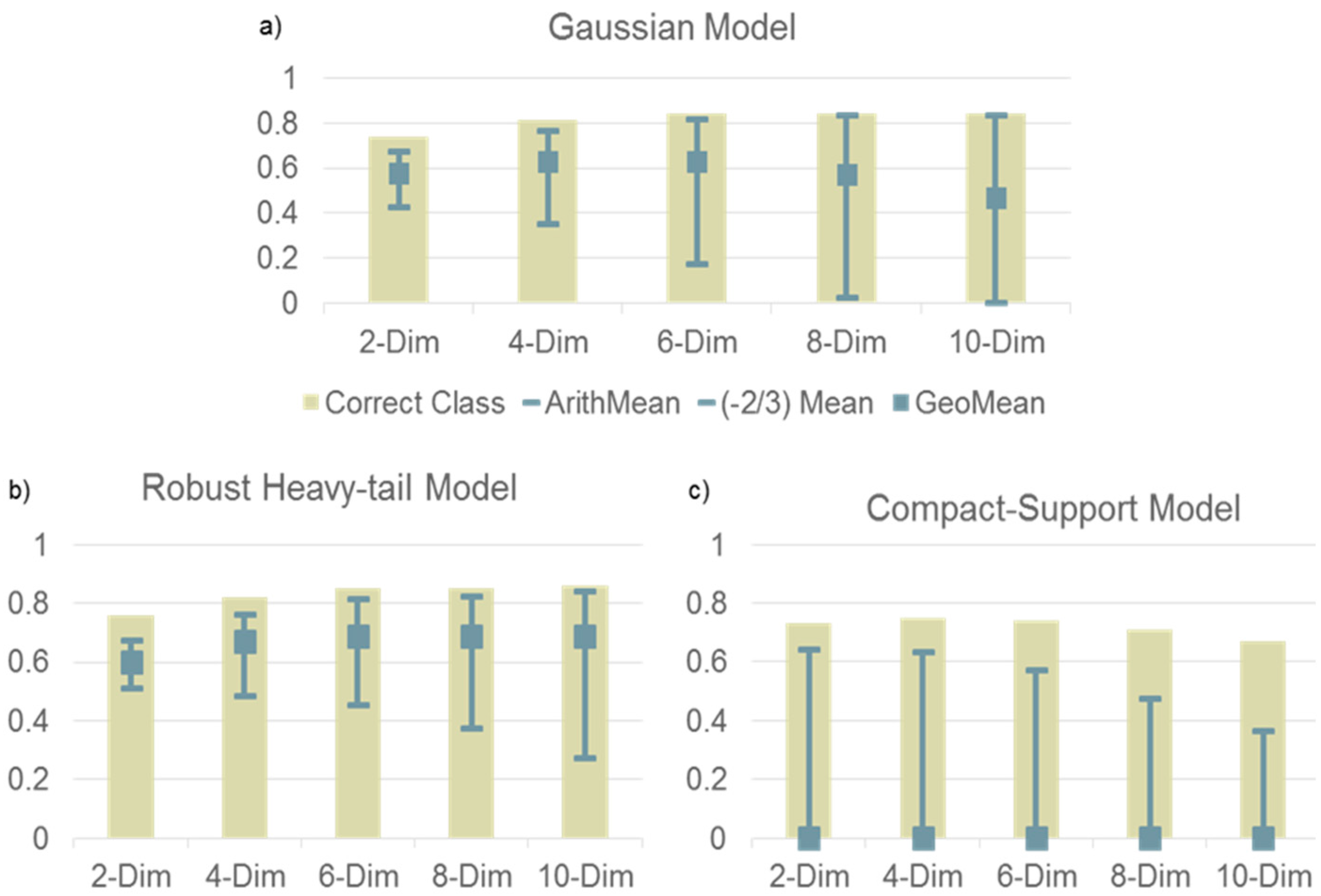
An example of how the generalized mean can be used to assess the performance of an inference model is illustrated Figure 1. In this example two 10-dimensional Gaussian distributions are sources for a set of random variables. The distributions have equal variance of 1 along each dimension and no correlation and are separated by a mean of one along each dimension. Three models of the uncertainty are compared. For each model 25 samples are used to estimate of the two means and single variance. The models vary the decay of the tail of a Coupled-Gaussian:

$$G_{\kappa }\left(x;\mathit{\mu },\mathsf{\Sigma }\right)\equiv \frac{1}{Z_{\kappa }\left(\mathsf{\Sigma }\right)}{\left(1+\kappa {\left(x-\mathit{\mu }\right)}^{⊺}\cdot {\mathsf{\Sigma }}^{-1}\cdot \left(x-\mathit{\mu }\right)\right)}_{+}^{-\frac{1}{2}\left(\frac{1}{\kappa }+d\right)},$$

(14)

where $\mathit{\mu }\mathrm{and}\mathsf{\Sigma }$ are the location vector and scale matrix, $\kappa$ is the degree of nonlinear coupling controlling the tail decay, d is the dimensions, Z is the normalization and ${(a)}_{+}=\max (0,a)$. In Figure 1a, the decay is Gaussian κ = 0. As more dimensions are modeled the accuracy of the classification performance (bar) and the accuracy of the reported probabilities (gray square at 0.63) measured by the geometric mean (m = 0) reach their maximum at six dimensions.

For eight and 10 dimensions, the classification does not improve and the probability accuracy degrades. This is because the estimation errors in the mean and variance eventually result in an over-fit model. The decisiveness (upper gray error bar) approximates the percentage of correct classification (light brown bar) and the robustness (lower gray error bar) goes to zero. In contrast b) the heavy-tail model with κ = 0.162 is able to maintain an accuracy of 0.69 for dimensions 6, 8 and 10. The heavy-tail makes the model less susceptible to over-fitting. For c) the compact-support model (κ = 0.095) even the 2-dimensional model has inaccurate probabilities (0), because a single probability report of zero, causes the geometric mean to be zero.

4. Comparing Probability Inference Performance with the Data Distribution

To better understand the sources of inaccuracy in a model, Equation (9) can be used to separate the error into the “source probability” of the underlying data source and the “divergence probability” between the model and the data source. Doing so requires an estimate of the source distribution of the data for a reported probability. This is accomplished using histogram analysis of the reported probabilities, though improved estimates are possible utilizing for example Bayesian priors for the bins, kernel methods, and k-nearest neighbor. In addition to the splitting of the components of the standard entropy measures, the generalized entropy equivalents using the generalized mean are also split into source and divergence components as described below. The histogram results and the overall metrics (arithmetic, geometric, and −2/3 mean) are visualized in a plot of the model probability versus source probabilities.

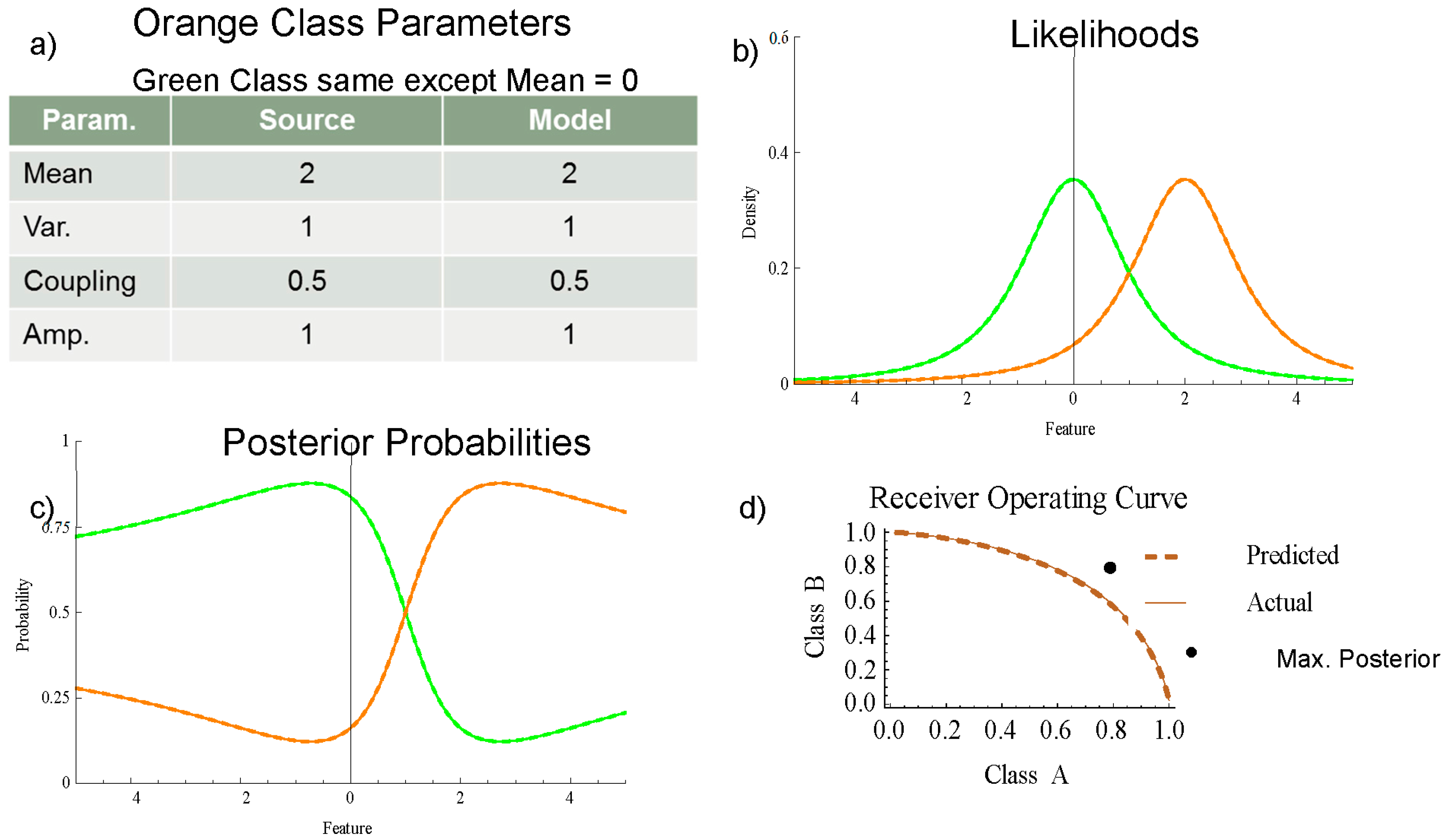
Figure 2 shows: (a) the parameters, (b) the likelihoods, (c) the posterior probabilities, and (d) the receiver operating characteristic (ROC) curve of a perfectly matched model for two classes with one-dimensional Coupled Gaussian distributions. The distribution data source in Figure 2c is shown as solid green and orange curves. Overlaying the source distribution is the model distributions shown as dashed curves. The heavy-tail decay (κ = 0.5) has the effect of keeping the posterior probabilities from saturating away from the mean shown in Figure 2c; instead, the posteriors return gradually to the prior distribution. The actual ROC curve in Figure 2d uses the model probabilities to classify and the source probabilities to determine the distribution. The predicted ROC curve uses the model probabilities for both the classification and calculation of the distribution.

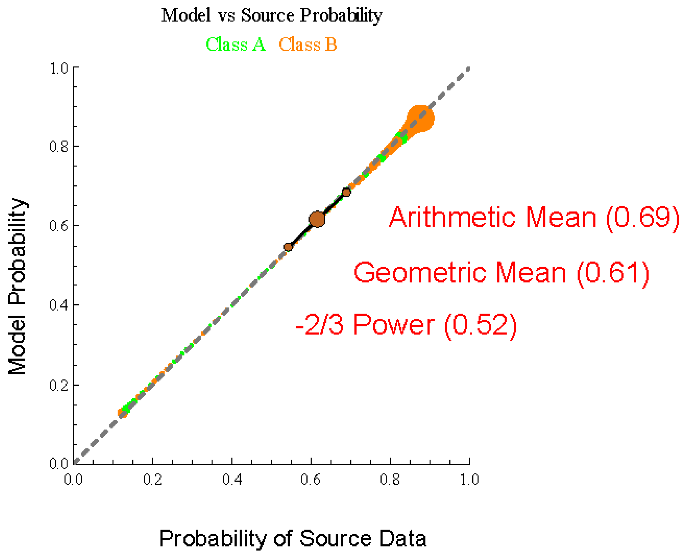
While the ROC curve is an important metric for assessing probabilistic inference algorithms, it does not fully capture the relationship between a model and the distribution of the test set. Figure 3 introduces a new quantitative visualization of the performance of a probabilistic inference. The approach builds upon histogram plots which are used to calibrate probabilities, shown as green and orange bubbles for each class. The histogram information is quantified into three metrics, the arithmetic mean (called Decisiveness), the geometric mean (called Accuracy) and the −2/3 mean (called Robustness), shown has brown marks. In the case of perfectly matched model with the source all the histogram bubbles and each of the metrics aligns along the 45 diagonal representing equality between the model probabilities and the source probabilities. In Section 5 illustrations will be provided which show how these metrics can show the gap in performance of a model, whether the model is under or over-confident, and the limitations to discrimination of the available information.

Because the goal is to maximize the overall performance of the algorithm, the model probability is shown on the y-axis. The distribution of the source or test data is treated as the independent variable on the x-axis. This orientation is reverse to common practice [19,20], which bins the reported probabilities and shows the distribution vertically; however, the adjustment is helpful for focusing on increasing model performance. In Figure 3 the orange and green bubbles are individual histogram data. Neighboring model probabilities for the green or orange class are grouped to form a bin. The y-axis location is the geometric mean of the model probabilities. The x-axis location is the ratio of the samples with the matching green or orange class divided by the total number of samples.

The process for creating model versus source probability plot given a test set of reported or model probabilities $Q=\left\{q_{ij}:i=\mathrm{1...}N,j=\mathrm{1...}M\right\}$, where i is the event number and j is the class label and $q_{ij*}$ is the labeled true event is as follows. There are some distinctions between the defined process and that used to create the simulated data in Figure 3 through Figure 6 which will be noted.

(1)

Sort data: The probabilities reported are sorted. As shown the sorting is separated by class, but could also be for all the classes. A precision limit $q_{\lim }$ is defined such that all the model probabilities satisfy $q_{\lim }\le q\le 1-q_{\lim }$.

(2)

Bin data: Bins with an equal amount of data are created to insure that each bin has adequate data for the analysis. Alternatively, cluster analysis could be completed to insure that each bin has elements with similar probabilities.

(3)

Bin analysis: For each bin k the average model probability, the source probability, and the contribution to the overall accuracy are computed.

(a)

Model probability (y-axis): Compute the arithmetic, geometric, and $-\raisebox{1ex}{$2$}\!\left/ \!\raisebox{-1ex}{$3$}\right.$ mean of the model probabilities for the actual event:

$$Q_k^{\left(m\right)}=\{\begin{array}{cc}{\displaystyle \prod _{i=1}^{N_k}{q}_{ij*k}^{1/N_k}}& m=0\\ {\left(\frac{1}{N_k}{\displaystyle \sum _{i=1}^{N_k}{q}_{ij*k}^m}\right)}^{\frac{1}{m}}& m=1,-\raisebox{1ex}{$2$}\!\left/ \!\raisebox{-1ex}{$3$}\right.,\end{array}$$

(15)

where m is the power of the weighted generalized mean.

(b)

Source probability (x-axis): Compute the frequency of true events in each bin:

$$P_k=\frac{{\displaystyle \sum _{j=1}^M{N}_{jk}^{\ast }}}{{\displaystyle \sum _{j=1}^M{N}_{jk}}},$$

(16)

where $N_{jk}\mathrm{and}{N}_{jk}^{\ast }$ are the number of j class element in bin k and the number of true j class elements in be k, respectively. If a source probability is calculated for each sample using k-nearest neighbor or kernel methods, then the arithmetic, geometric, and $-\raisebox{1ex}{$2$}\!\left/ \!\raisebox{-1ex}{$3$}\right.$ mean can also be calculated for the source probabilities.

(c)

Contribution to overall accuracy (size): Figure 3 through Figure 6 show bubble sizes proportional to the number of true events; however, a more useful visualization is the contribution each bin makes to the overall accuracy. This is determined by weighting the model average by the source average. Taking the logarithm of this quantity makes a linear scale for the bubble size:

$$\left(\raisebox{1ex}{$\frac{{\displaystyle \sum _{j=1}^M{N}_{j*k}}}{{\displaystyle \sum _{j=1}^M{N}_{jk}}}$}\!\left/ \!\raisebox{-1ex}{${\displaystyle \sum _{k=1}^b\frac{{\displaystyle \sum _{j=1}^M{N}_{j*k}}}{{\displaystyle \sum _{j=1}^M{N}_{jk}}}}$}\right.\right)\ln \left({\displaystyle \prod _{i=1}^{N_{j*k}}{q}_{ij*k}^{1/N_{j*k}}}\right)$$

(17)

(4)

Overall Statistics: The overall statistics are determined by the generalized mean of the individual bin statistics.

(a)

Overall Model Statistics:

$${\left(\frac{1}{B}{\displaystyle \sum _{k=1}^B{\left(\frac{1}{N_k}{\displaystyle \sum _{i=1}^{N_k}{q}_{ij*k}^m}\right)}^{\xcancel{\frac{m}{m}}}}\right)}^{\frac{1}{m}},$$

(18)

where B is the number of bins.

(b)

Overall Source Statistics:

$${\left(\frac{1}{B}{{\displaystyle \sum _{k=1}^B\left(\frac{{\displaystyle \sum _{j=1}^M{N}_{jk}^{\ast }}}{{\displaystyle \sum _{j=1}^M{N}_{jk}}}\right)}}^m\right)}^{\frac{1}{m}}$$

(19)

In Figure 3 through Figure 6 the brown marks are located at the (x, y) point corresponding to the (model, source) mean for the three metrics Decisiveness (arithmetic, m = 1), Accuracy (geometric, m = 0), and Robustness (m = −2/3).

5. Effect of Model Errors in Mean, Variance, Shape, and Amplitude

The three metrics (Decisiveness, Accuracy, and Robustness) provide insight about the discrepancy between an inference model and the source data. The accuracy (geometric mean) always degrades due to errors, while the changes in the decisiveness and robustness provide an indication of whether an algorithm is under or over-confident. The discrepancy in accuracy will be quantified as the “probability divergence” using Equation (8) and discussed more thoroughly in Section 6. The effect of four errors (mean, variance, shape, and amplitude) on one of the two class models will be examined.

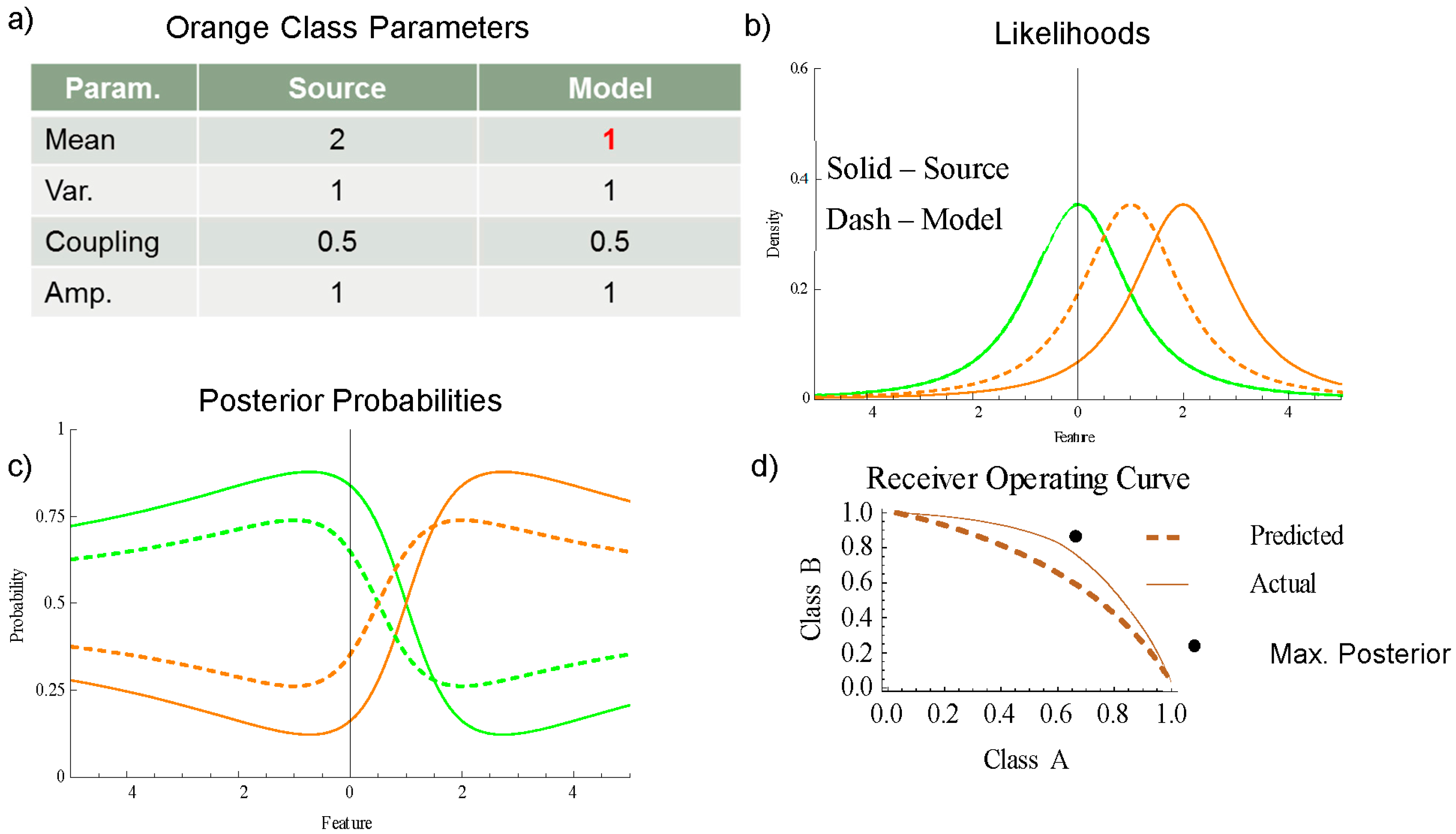
In Figure 4 the mean of the model (a) is shifted from 2 to 1 for the orange class. The closer spacing of the hypotheses shown in (b) results in under-confident posterior probabilities shown in (c), where the dashed curves of the model are closer to 0.5 than the solid source curves. The actual ROC curve shown as a solid curve in (d) is better than the forecasted ROC curve (dashed). Each histogram bin for the analysis is a horizontal slice of the neighboring probabilities in Figure 4c. A source of error in estimating the source probabilities is that model probabilities are drawn from multiple features; two in one-dimensional single modal distributions used here for demonstration. For more complex distributions with many modes and/or many dimensions the analysis would have to be segmented by feature regions.

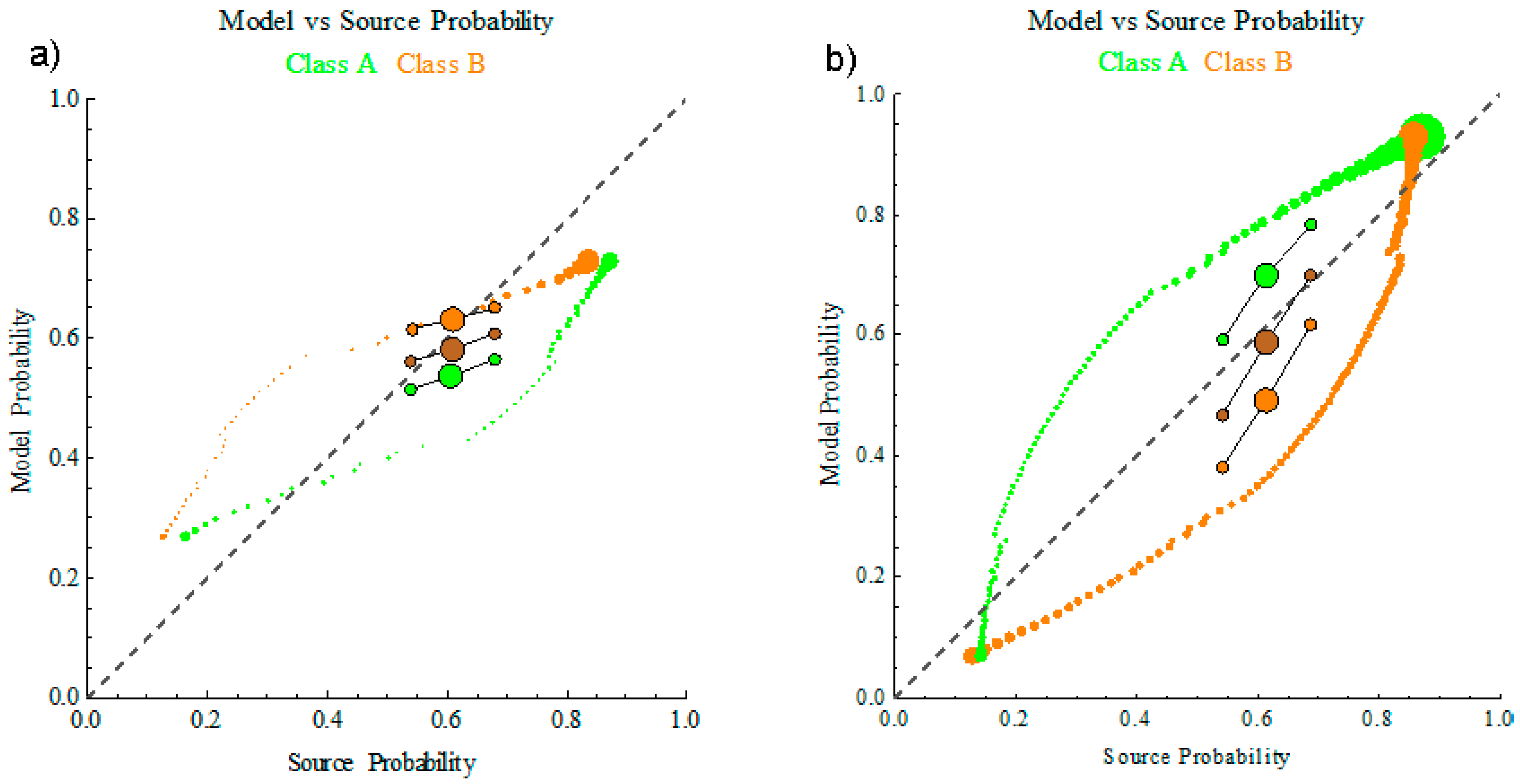
Figure 5a shows how the under-confident model affects the model probability versus the source probability plot. The green and orange class bubbles separate. For source probabilities greater/less than 0.5 the model probabilities tend to be lower/higher, reflecting the higher uncertainty reported by the model. The large brown mark, which represents the average probability reported by the model versus the average probability of the source distribution, is below the equal probability dashed line due to the error in the model. The decisiveness and robustness metrics (smaller brown marks) have an orientation with the x-axis which is less than 45°, indicative of the model being less decisive but more robust (i.e., smaller variations in the reported uncertainty). The decisive metric, which is the arithmetic mean, has a larger average, while the robust metric, which is the −2/3 mean, has a smaller average. Figure 5b shows the contrasting result when the orange class model has an over-confident mean shifted from 2 to 3. The orange and green class bubbles now have average model probabilities which are more extreme than the source probabilities. The overall reported probabilities still decreases relative to a perfect model (large brown mark), but the orientation of the decisive and robust metrics is now greater than 45°.

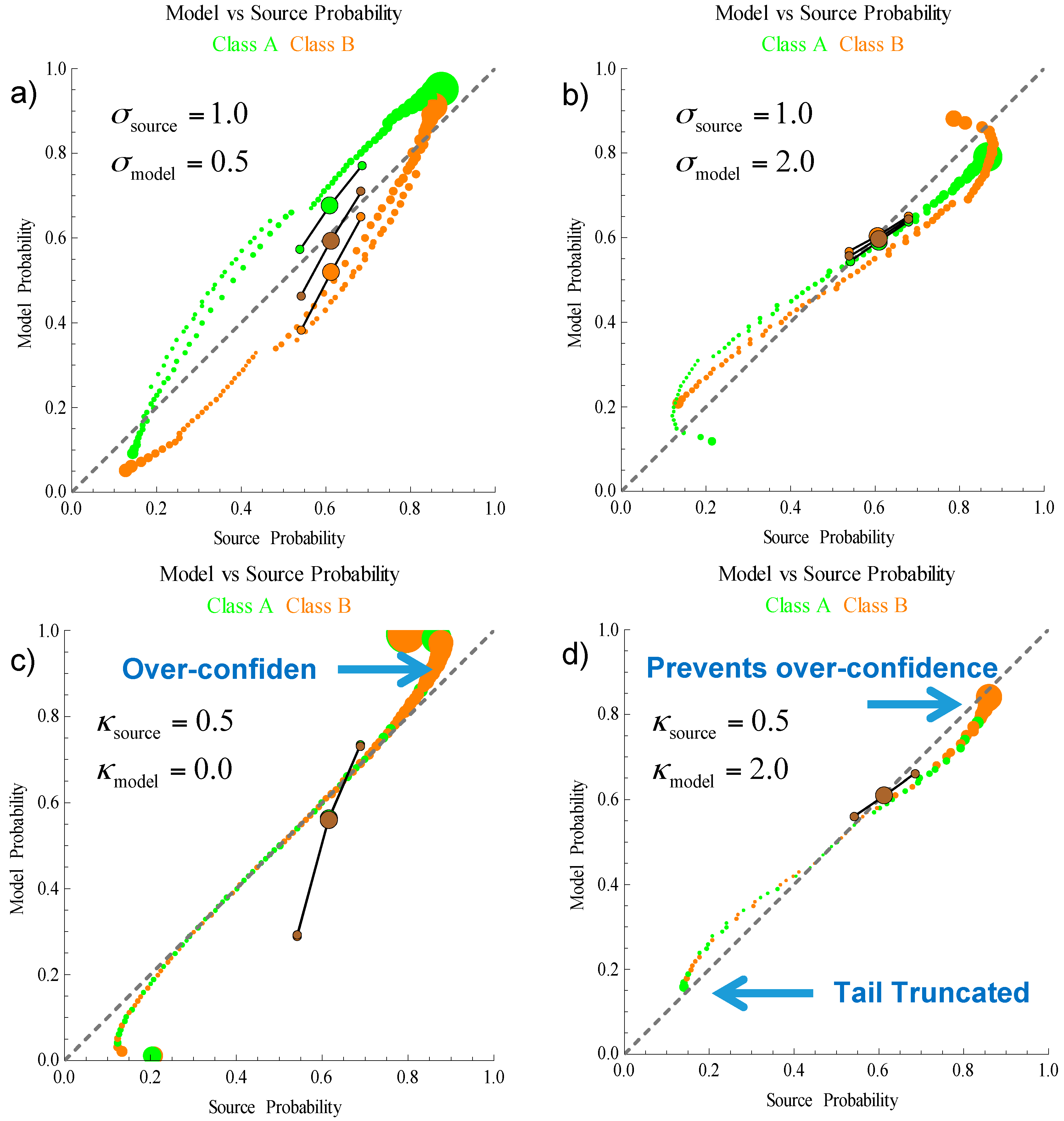
Other model errors have a similar effect in lowering the model average below equality with the source average, and shifting the orientation of the decisiveness and robustness to be greater or less than 45°. The full spectrum of the generalized mean may provide approaches for more detailed analysis of an algorithms performance, but will be deferred. In Figure 6 the effect of under and over-confident variance and tail decay are shown. When the model variance is inaccurate (a) and (b) the changes to the three metrics are similar to the effect of an inaccurate mean. The model accuracy decreases and the angle of orientation for the decisive/robust metrics increases or decreases for over or under confidence. When the tail decay is over-confident (c) the probabilities in the middle of the distribution are accurate, but the tail inaccuracy can significantly increase the angle of orientation of the decisive/robust metrics. When the tail decay is under-confident (d) the probabilities are truncated near the extremes of 0 and 1. An under-confident model of the tails, can be beneficial in providing robustness against other errors.

6. The Divergence Probability as a Figure of Merit

The accuracy of a probabilistic inference, measured by the source probability, as described in the previous sections, is affected by two sources of error, the uncertainty in the distribution of the source data and the divergence between the model and source distributions. The divergence can be isolated by dividing out the probability associated with the source from the model probability. This is a rearrangement of Equation (9) $P_{Div}\left(p_{j*}\Vert q_{j*}\right)=P_{Model}\left(p_{j*},q_{j*}\right)/P_{Source}\left(p_{j*}\right),$ $p_{j*}$ is the vector of true state reported probabilities and $q_{j*}$ is the vector of estimated source probabilities. The divergence probability can be utilized as a figure of merit regarding the degree of confidence in an algorithms ability to report accurate probabilities. The source probability reflects the uncertainty in the data source based on issues such as the discrimination power of the features.

Figure 7 shows a geometric visualization of the divergence probability for the example when the tail is over-confident (model κ = 0 and source κ = 0.5). The model probability corresponds to the y-axis location of the algorithm accuracy shown as a brown mark. The source probability is the x-axis location of the accuracy. The ratio of these two quantities (divergence probability) is equivalent to projecting the y-axis onto the point where the x-axis is length 1. The resulting quantities are $P_{Model}\left(p_{j*},q_{j*}\right)=0.56,$ $P_{Source}\left(p_{j*}\right)=0.62,$ and $P_{Div}\left(p_{j*}{\Vert q}_{j*}\right)=P_{Model}\left(p_{j*},q_{j*}\right)/P_{Source}\left(p_{j*}\right)=\mathrm{0.90.}$

7. Discussion

The role and importance of the geometric mean in defining the average probabilistic inference has been shown through a derivation from information theory, a proof using Bayesian analysis, and via examples of a simple two-class inference problem. The geometric mean of a set of probabilities can be understood as the central tendency because probabilities, as ratios, reside on a multiplicative rather than an additive scale.

Two issues have limited the role the geometric mean as an assessment of the performance of probabilistic forecasting. Firstly, information theoretic results have been framed in terms of the arithmetic mean of the logarithm of the probabilities. While optimizing the logarithmic score is mathematically equivalent to optimizing the geometric mean of the probabilities, use of the logarithmic scale obscures the connection with the original set of probabilities. Secondly, because the log score and the geometric mean are very sensitive averages, algorithms which do not properly account for the role of tail decay in achieving accurate models suffer severely against these metrics. Thus metrics, such as the quadratic mean, which keep the score for a forecast of $p=0$ finite and are made proper by subtracting the bias, have been attractive alternatives.

Two recommendations are suggested when using the geometric mean to assess the average performance of a probabilistic inference algorithm. First, careful consideration of the tail decay in the source of the data should be accounted for in the models. Secondly, a precision should be specified which restricts the reported probabilities to the range of $q_{\lim }\le q\le 1-q_{\lim }.$ Unlike an arithmetic scale, on the multiplicative scale of probabilities precision affects the range of meaningful quantities. In the examples visualizing the model versus source probabilities, the precision is $q_{\lim }=0.01$ and matches the bin widths. The issue of precision is particularly important when forecasting rare events. Assessment of the accuracy needs to consider the size of the available data and how this affects the precision which can be assumed.

The role of the quadratic score can be understood to include an assessment of the “Decisiveness” of the probabilities rather than purely the accuracy. In the approach described here this is fulfilled by using the arithmetic mean of the true state probabilities. Removing the bias in the arithmetic mean via incorporation of the non-true state probabilities is equivalent to the quadratic score; however, by keeping it a local mean the method is simplified and insight is provided regarding the degree of fluctuation in the reported probabilities.

Balancing the arithmetic mean, the −2/3 mean provides an assessment of the “Robustness” of the algorithm. In this case, the metric is highly sensitive to reported probabilities of the actual event which are near zero. This provides an important assessment of how well the algorithm minimizes fluctuations in reporting the uncertainty and provides robustness against events which may not have been included in the testing. Together the arithmetic and −2/3 metrics provide an indication of the degree of variation around the central tendency measure by the geometric mean.

The performance of an inference algorithm, including its tendency for being under or over-confident can be visualized by plotting the model versus source averages. As just described, the model averages are based on the generalized mean of the actual events. The contribution to the uncertainty from the source is determined by binning similar forecasts. The source probability for each bin is the frequency of probabilities associated with a true event in each bin. The arithmetic, geometric, and −2/3 means of the source probability for each bin are used to determine the overall source probability means. The geometric mean of the model probabilities is called the model probability and is always less than the source probability. The ratio of these quantities is the divergence probability, Equation (9), and is always less than one.

A perfect model has complete alignment between the source and model probabilities, and in turn the three metrics are aligned along the 45° line of the model versus source probability plot. If the algorithm is over-confident the arithmetic mean of the reported probabilities increases and the −2/3 mean decreases, causing a rotation in the orientation of the three metrics to a higher angle. In contrast an under-confident algorithm causes a rotation to a lower angle. This was illustrated using a two-class discrimination problem as an example, showing the effects of errors in the mean, variance, and tail decay. The three metrics provide a quantitative measure of the algorithms performance as a probability and an indication of whether the algorithm is under or over confident. Distinguishing between the types of error (mean, variance, and decay) may be possible by analyzing the full spectrum of the generalized mean and is recommended for future investigations.

References

- Jose, V.R.R.; Nau, R.F.; Winkler, R.L. Scoring rules, generalized entropy, and utility maximization. Oper. Res. 2008, 56, 1146. [Google Scholar] [CrossRef]
- Jewson, S. The problem with the Brier score. arXiv 2004. [Google Scholar]
- Ehm, W.; Gneiting, T. Local Proper Scoring Rules; Department of Statistics, University of Washington: Seattle, WA, USA, 2009. [Google Scholar]
- Gneiting, T.; Raftery, A.E. Strictly proper scoring rules, prediction, and estimation. J. Am. Stat. Assoc. 2007, 102, 359–378. [Google Scholar] [CrossRef]
- Dawid, A.P. The geometry of proper scoring rules. Ann. Inst. Stat. Math. 2007, 59, 77–93. [Google Scholar] [CrossRef]
- Dawid, A.; Musio, M. Theory and applications of proper scoring rules. Metron 2014. [Google Scholar] [CrossRef]
- Fleming, P.J.; Wallace, J.J. How not to lie with statistics: The correct way to summarize benchmark results. Commun. ACM 1986, 29, 218–221. [Google Scholar] [CrossRef]
- McAlister, D. The law of the geometric mean. Proc. R. Soc. Lond. 1879, 29, 367–376. [Google Scholar] [CrossRef]
- Khinchin, A.I. Mathematical Foundations of Information Theory; Courier Corporation: North Chelmsford, MA, USA, 1957. [Google Scholar]
- Bernardo, J.M.; Smith, A.F.M. Inference and Information. In Bayesian Theory; John Wiley & Sons: Hoboken, NJ, USA, 2009; pp. 67–81. [Google Scholar]
- Shannon, C.E.; Weaver, W. The Mathematical Theory of Communication; University of Illinois Press: Urbana, IL, USA, 1949; p. 114. [Google Scholar]
- Cover, T.M.; Thomas, J.A. Elements of Information Theory; John Wiley & Sons: Hoboken, NJ, USA, 2012. [Google Scholar]
- Huber, P.J.; Ronchetti, E.M. Robust Statistics, 2nd ed.; John Wiley & Sons: Hoboken, NJ, USA, 2009. [Google Scholar]
- Rényi, A. On measures of entropy and information. Proc. Fourth Berkeley Symp. Math. Stat. Probab. 1961, 1, 547–561. [Google Scholar]
- Tsallis, C. Nonadditive entropy and nonextensive statistical mechanics—an overview after 20 years. Braz. J. Phys. 2009, 39, 337–356. [Google Scholar] [CrossRef]
- Nelson, K.P.; Scannell, B.J.; Landau, H. A Risk Profile for Information Fusion Algorithms. Entropy 2011, 13, 1518–1532. [Google Scholar] [CrossRef]
- Oikonomou, T. Tsallis, Renyi and nonextensive Gaussian entropy derived from the respective multinomial coefficients. Phys. A Stat. Mech. Appl. 2007, 386, 119–134. [Google Scholar] [CrossRef]
- Nelson, K.P.; Umarov, S.R.; Kon, M.A. On the average uncertainty for systems with nonlinear coupling. Phys. A Stat. Mech. Its Appl. 2017, 468, 30–43. [Google Scholar] [CrossRef]
- Cohen, I.; Goldszmidt, M. Properties and benefits of calibrated classifiers. Lect. Notes Comput. Sci. 2004, 3202, 125–136. [Google Scholar]
- Niculescu-Mizil, A.; Caruana, R. Predicting good probabilities with supervised learning. In Proceedings of the 22nd International Conference on Machine Learning ICML 05, Bonn, Germany, 7–11 August 2005; pp. 625–632. [Google Scholar]
Figure 1.
Source of random variables are two independent 10 dimensional Gaussian. The model estimates the mean and variance of each dimension using 25 samples. The mean and variance are used as the location and scale for three Coupled-Gaussian models, (a) κ = 0 Gaussian, (b) κ = 0.162 Heavy-tail (c) κ = 0.095 Compact-support.
Figure 2.
A two-class classification example with single-dimension Coupled Gaussian distributions. (a) The parameters for the orange class source and model are shown; (b) The likelihood distributions are shown. The solid (source) and dashed (model) overlap in this case, representing a perfectly matched model; (c) The posterior probabilities assuming equal priors for each class; (d) The receiver operating characteristic curve (solid) and a “predicted” ROC curve (dashed), which is determined using only the model distributions.
Figure 3.
The average model probability versus the average source probability for the model/source of Figure 1. The orange and green bubbles represent individual bins, with bins grouped by the model probability and the ratio of class to total distribution represented by the source probability. The brown marks are the overall averages (arithmetic, geometric, and −2/3). For a perfect model all are on the identity.
Figure 4.
(a,b) The orange model (dashed line) has mean of 1 rather than the source of mean 2. The results in (c) under-confident posterior probabilities and a shift in the maximum posterior decision boundary. (d) While the ROC curve and Maximum Posterior classification performance are only modified slightly from the performance of the perfect model, the predicted ROC curve shows a significant discrepancy.
Figure 5.
The model probability versus source probability for (a) the under-confident mean model pictured in Figure 4 and (b) an over-confident mean model. The green and orange class bubbles separate along with the three averages for each class. The large brown mark is the overall accuracy which is now below the dashed line for both the under and over-confident models. For (a) the alignment of the three overall metrics (brown) is less than 45° indicating under-confidence. For (b) the alignment of the three overall metrics is greater than 45° indicating over-confidence.
Figure 6.
The model versus source average probability when the orange class variance model is over or under confident. (a) The orange model has a variance 0.5 rather than the source variance of 1.0. The model accuracy (large brown mark) is lower than the source accuracy and the orientation of the decisive/robust metrics (smaller brown marks) is greater than 45°; (b) When the variance is over-confident (2.0) the accuracy also decreases and the decisive/robust orientation is less than 45°; (c) The coupling or tail decay of the model is over-confident. is a Gaussian distribution. Only the probabilities near 0 or 1 are inaccurate, but this significantly increases the orientation of the decisive/robust metrics angle above 45°; (d) When the tail model is under-confident reported probabilities near 0 or 1 are truncated. This can provide robustness against other sources of errors.
Figure 7.
The accuracy of an inference algorithm measured by the model probability (y-axis) consists of two components, the source probability (x-axis) and the divergence probability (projection of the cross-entropy probability onto the 0 to 1 scale).
© 2017 by the author. Licensee MDPI, Basel, Switzerland. This article is an open access article distributed under the terms and conditions of the Creative Commons Attribution (CC BY) license (http://creativecommons.org/licenses/by/4.0/).
Share and Cite
MDPI and ACS Style
Nelson, K.P. Assessing Probabilistic Inference by Comparing the Generalized Mean of the Model and Source Probabilities. Entropy 2017, 19, 286. https://0-doi-org.brum.beds.ac.uk/10.3390/e19060286
AMA Style
Nelson KP. Assessing Probabilistic Inference by Comparing the Generalized Mean of the Model and Source Probabilities. Entropy. 2017; 19(6):286. https://0-doi-org.brum.beds.ac.uk/10.3390/e19060286
Chicago/Turabian StyleNelson, Kenric P. 2017. "Assessing Probabilistic Inference by Comparing the Generalized Mean of the Model and Source Probabilities" Entropy 19, no. 6: 286. https://0-doi-org.brum.beds.ac.uk/10.3390/e19060286
Note that from the first issue of 2016, this journal uses article numbers instead of page numbers. See further details here.