Encryption Algorithm of Multiple-Image Using Mixed Image Elements and Two Dimensional Chaotic Economic Map


1
Department of Mathematics, Faculty of Science, Mansoura University, Mansoura 35516, Egypt
2
Computer Science Unit, Deanship of Educational Services, Qassim University, P.O. Box 6595, Buraidah 51452, Saudi Arabia
Entropy 2018, 20(10), 801; https://0-doi-org.brum.beds.ac.uk/10.3390/e20100801
Submission received: 15 September 2018
/
Revised: 15 October 2018
/
Accepted: 16 October 2018
/
Published: 18 October 2018
(This article belongs to the Special Issue Entropy in Image Analysis)
Abstract
:To enhance the encryption proficiency and encourage the protected transmission of multiple images, the current work introduces an encryption algorithm for multiple images using the combination of mixed image elements (MIES) and a two-dimensional economic map. Firstly, the original images are grouped into one big image that is split into many pure image elements (PIES); secondly, the logistic map is used to shuffle the PIES; thirdly, it is confused with the sequence produced by the two-dimensional economic map to get MIES; finally, the MIES are gathered into a big encrypted image that is split into many images of the same size as the original images. The proposed algorithm includes a huge number key size space, and this makes the algorithm secure against hackers. Even more, the encryption results obtained by the proposed algorithm outperform existing algorithms in the literature. A comparison between the proposed algorithm and similar algorithms is made. The analysis of the experimental results and the proposed algorithm shows that the proposed algorithm is efficient and secure.
Keywords:
image encryption; multiple-image encryption; two-dimensional chaotic economic map; security analysisMSC:
68U10; 68P25; 94A601. Introduction
A huge number of images are produced in many fields, such as weather forecasting, military, engineering, medicine, science and personal affairs. Therefore, with the fast improvement of computer devices and the Internet, media security turns into a challenge, both for industry and academic research. Image transmission security is our target. Many authors have proposed many single-image encryption algorithms to solve this problem [1,2,3,4,5,6,7,8]. Single-image encryption algorithms involve those using a chaotic economic map [1,2], using a chaotic system [3], via one-time pads-a chaotic approach [4], via pixel shuffling and random key stream [5], using chaotic maps and DNA encoding [6] and using the total chaotic shuffling scheme [7]. In [8], the authors proposed two secret sharing approaches for 3D models using the Blakely and Thien and Lin schemes. Those approaches reduce share sizes and remove redundancies and patterns, which may ease image encryption. The authors in [9] concluded that the dynamic rounds chaotic block cipher can guarantee the security of information transmission and realize a lightweight cryptographic algorithm. A single-image can encrypt multiple images repeatedly, but the efficiency of that encryption is always unfavorable. Researchers have increased their attention towards multiple-image encryption because a high efficiency of secret information transmission is required for modern multimedia security technology. Many multiple-image algorithms have been presented. The authors of [10] presented a multiple-image algorithm via mixed image elements and chaos. A multiple-image algorithm using the pixel exchange operation and vector decomposition was proposed in [11]. In [12], the authors presented an algorithm using mixed permutation and image elements. The authors presented multiple-image encryption via computational ghost imaging in [13]. In [14], the authors proposed an algorithm using an optical asymmetric key cryptosystem. A multiple-image encryption algorithm based on spectral cropping and spatial multiplexing was presented in [15]. The authors of [16] proposed a multiple-image encryption algorithm based on the lifting wavelet transform and the XOR operation based on compressive ghost imaging scheme. Even with this large number of proposed algorithms, some practical problems still exist. For instance, some multiple-image algorithms have faced the problem that the original images cannot be recovered completely [17,18,19]. Those algorithms were used to encrypt multiple images, but the corresponding original images were not recovered completely. This leads to lossy algorithms, which are not appropriate for those applications needing images with high visual quality. Another problem is that the complex computations of some algorithms affect the encryption efficiency [20,21]. Therefore, good techniques are required for solving these problems [22]. In the current paper, a new efficient multiple-image encryption algorithm using mixed image elements (MIES) and a two-dimensional chaotic economic map is proposed. The advantages of this algorithm are that it is able to recover plain images completely and simplifies the computations. Experimental results demonstrate its practicality and high proficiency.
The rest of the paper is organized as follows. The pure image elements (PIES) and the MIES are defined in Section 2. In Section 3, a brief introduction to the two-dimensional chaotic economic map is presented. The secret key generation is presented in Section 4. In Section 5, a new encryption algorithm of multiple images is designed. Experimental results and analyses are introduced in Section 6. Section 7 presents a comparison between the proposed algorithm and the identical algorithms. Conclusions are given in Section 8.
2. PIES and MIES
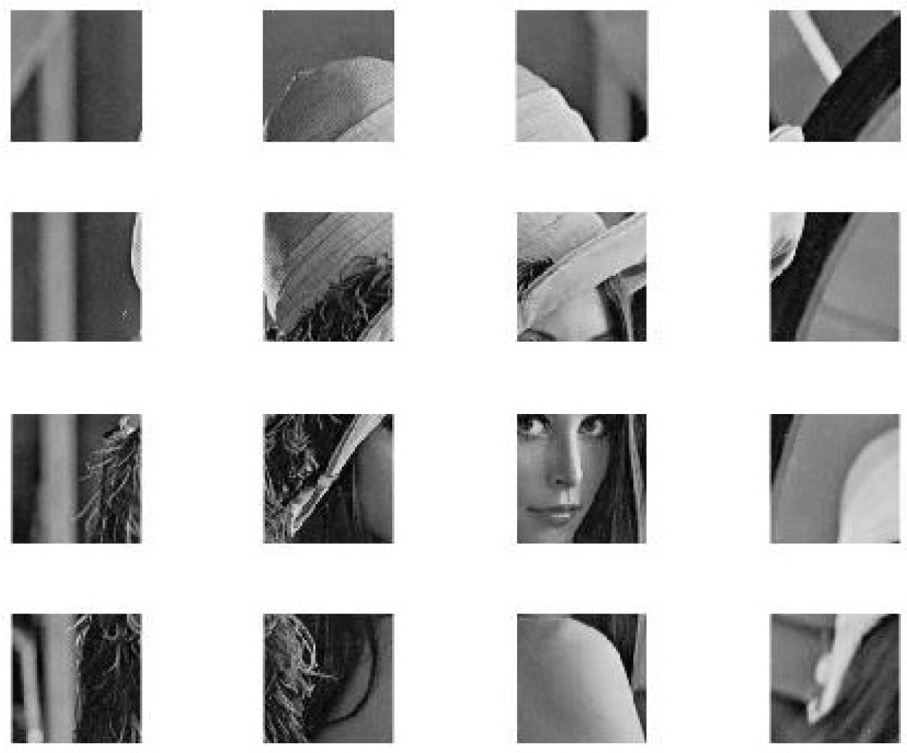
Matrix theory can be used to divide a big matrix into many small matrices and vice versa. Furthermore, in the image processing field, it is simple to divide an image into many small images and vice versa. For instance, Figure 1 can be divided into 16 small images with an equal size, as displayed in Figure 2. Therefore, the original image can be retrieved from these 16 images.
Assume that are k original images. can be divided into a small images set, . Each element is referred to as the pure image element. On the other hand, k sets of PIES , , ⋯, can be created, which correspond to , respectively. A large set can be obtained by mixing all PIES together. Each element is referred to as the mixed image element.
The current paper presents a new encryption algorithm of multiple images using MIES and the two-dimensional chaotic economic map. The secret key is very important to restore the original images from the MIES.
3. The Two-Dimensional Chaotic Economic Map
The study of the following two-dimensional chaotic economic system (dynamical system) was introduced in [23]:
where:
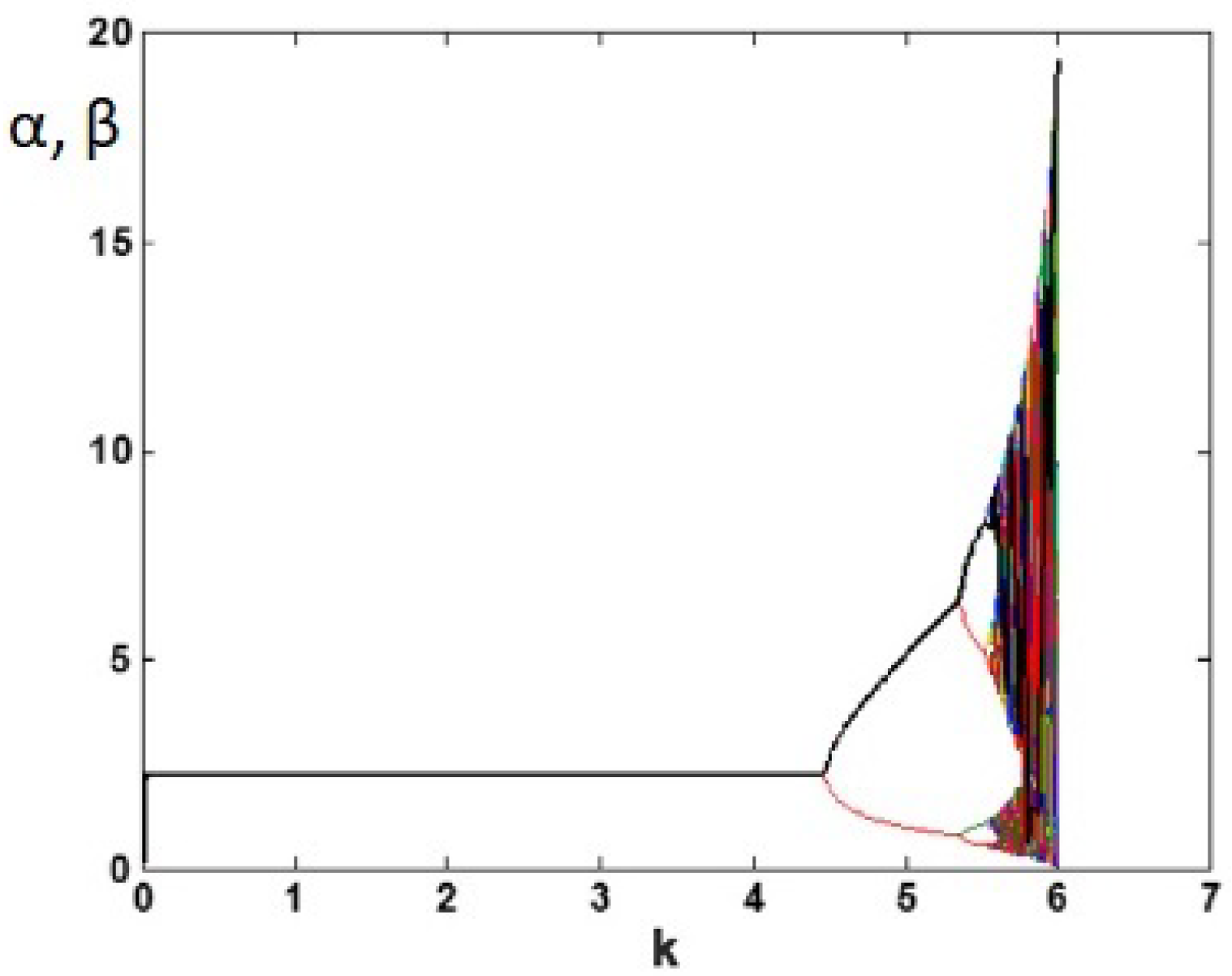
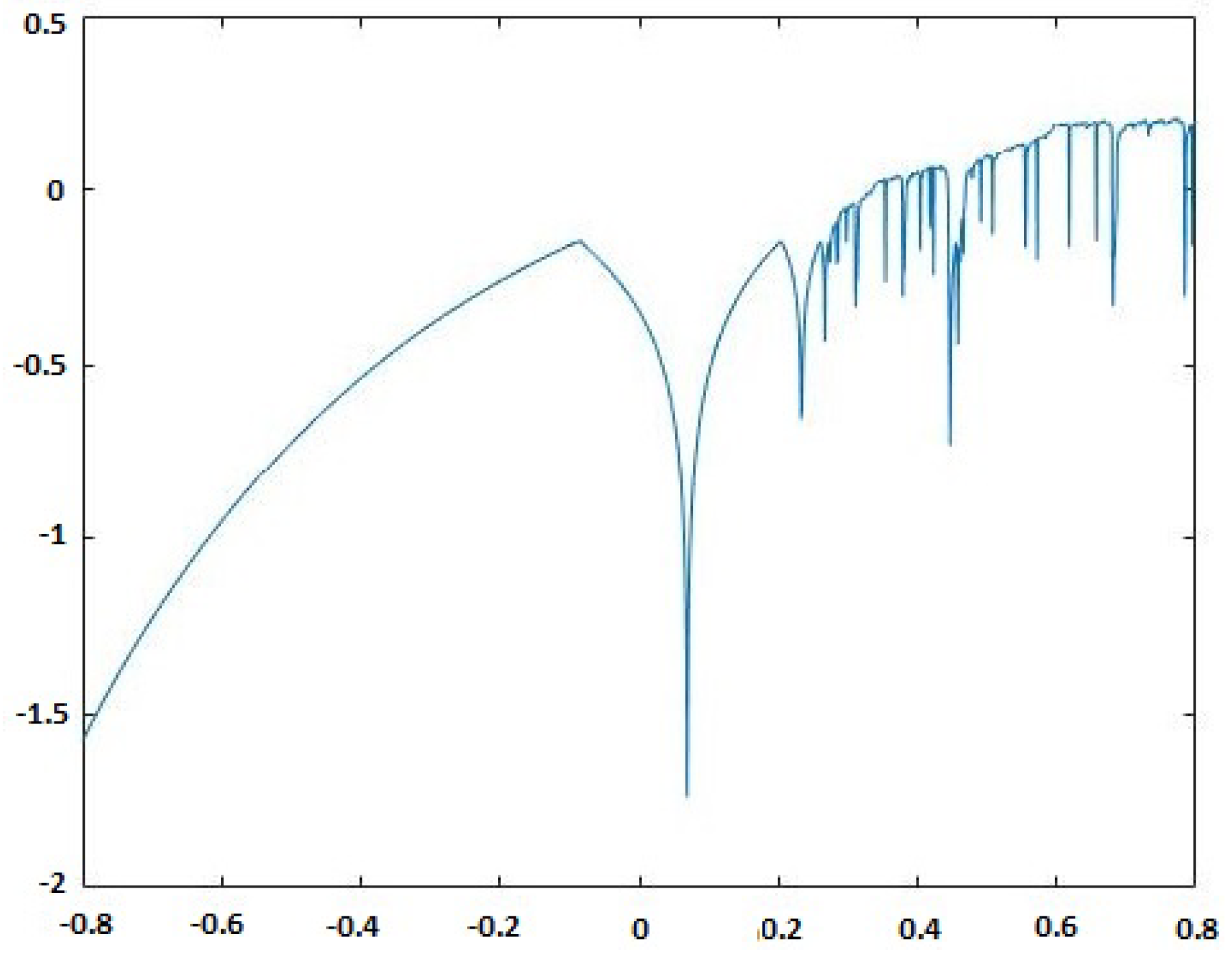
There are six parameters in the chaotic economic map (1). These parameters have economic significance; the parameter is used to capture the economic market size, while the market price slope is referred to by the parameter . To obtain a chaotic region, a must be greater than b and c. A fixed marginal cost parameter is denoted by , and the speed of adjustment parameter . The chaotic behavior of the chaotic economic map (1) at and is shown in Figure 3. In the current paper, the parameters and of the map (1) have been chosen in the chaotic region having positive Lyapunov exponents, as displayed in Figure 4.
4. The Secret Key Generation
Let , , be the big image created by combining the k original images of size , where refers to the pixel value at the position and is the size of the big image . The key mixing proportion factor can be used to calculate as follows:
Then, update the initial condition using the following formula:
where and , receptively.
After that, take four initial values, , four parameters for the logistic map, , two initial values for the system, , and four system parameters, .
5. The Proposed Multiple-Image Algorithm
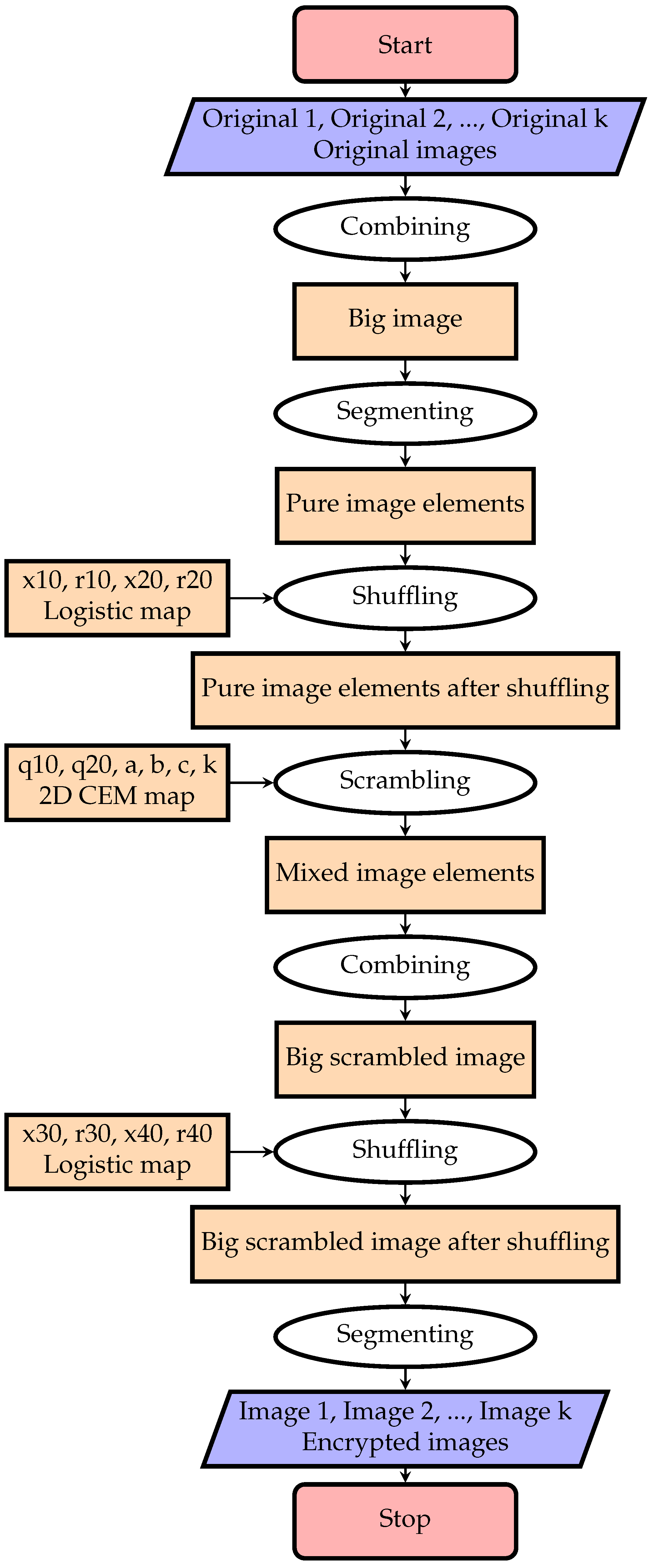
To encrypt multiple images jointly, the current work presents a new encryption algorithm of multiple images using MIES and the two-dimensional chaotic economic map. The flowchart of the new encryption algorithm is shown in Figure 5.
The proposed algorithm is processed as follows:
In the multiple-image decryption, the same chaotic economic sequences are generated on the multiple-image encryption that will be used to recover the original images and using the inverse steps of Algorithm 1.
| Algorithm 1 Multiple-image encryption |
|
6. Experimental Results and Analyses
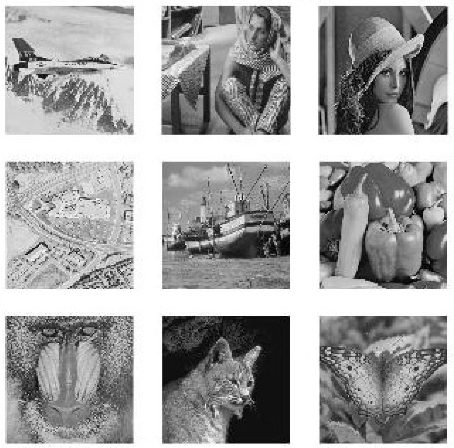
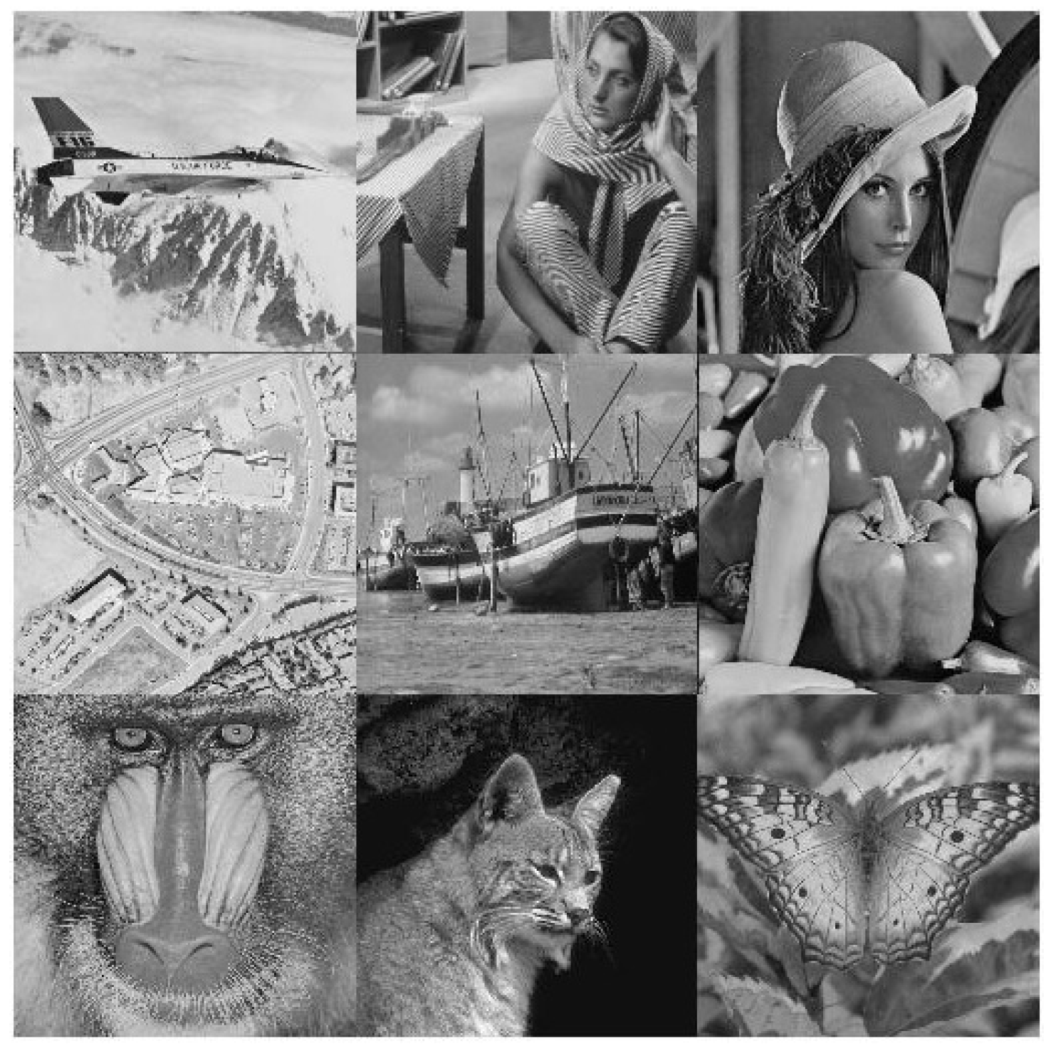
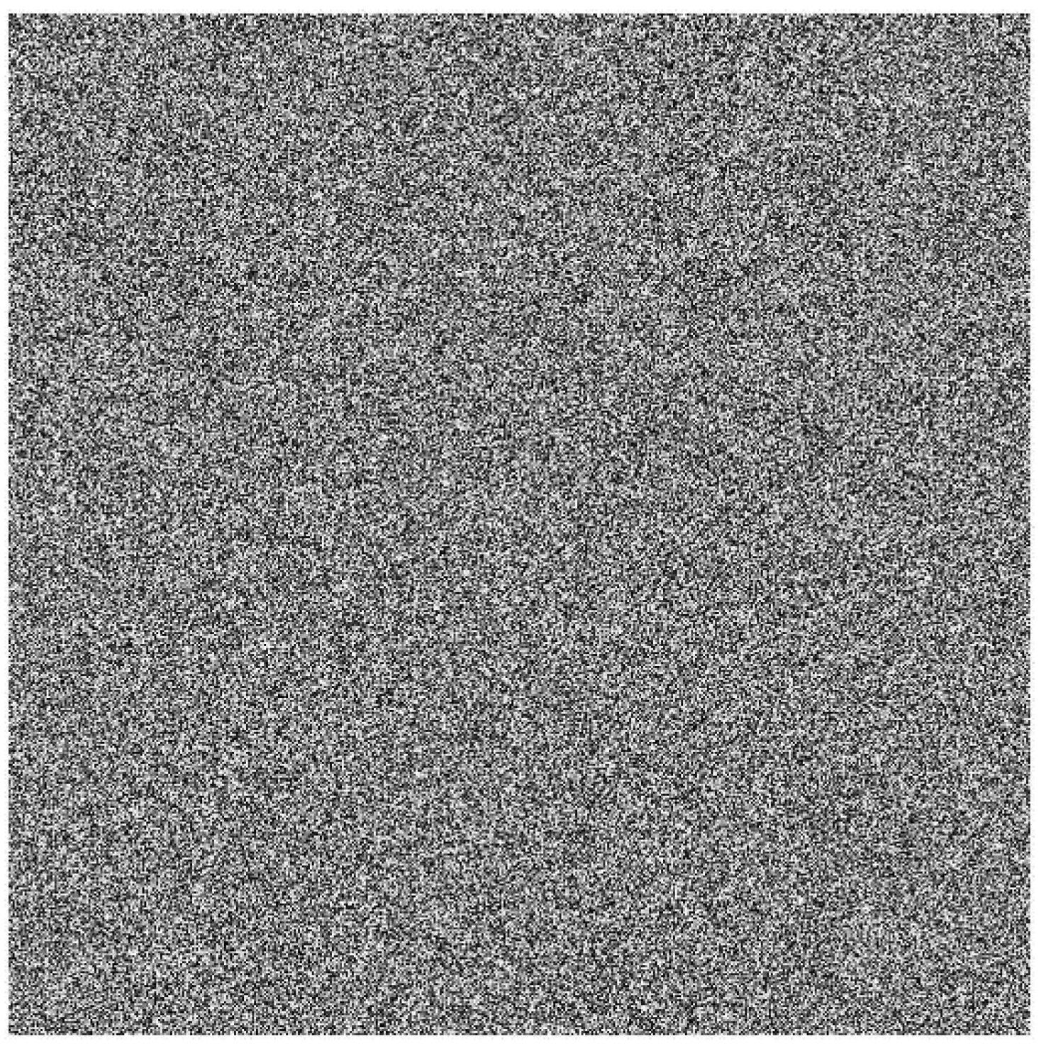
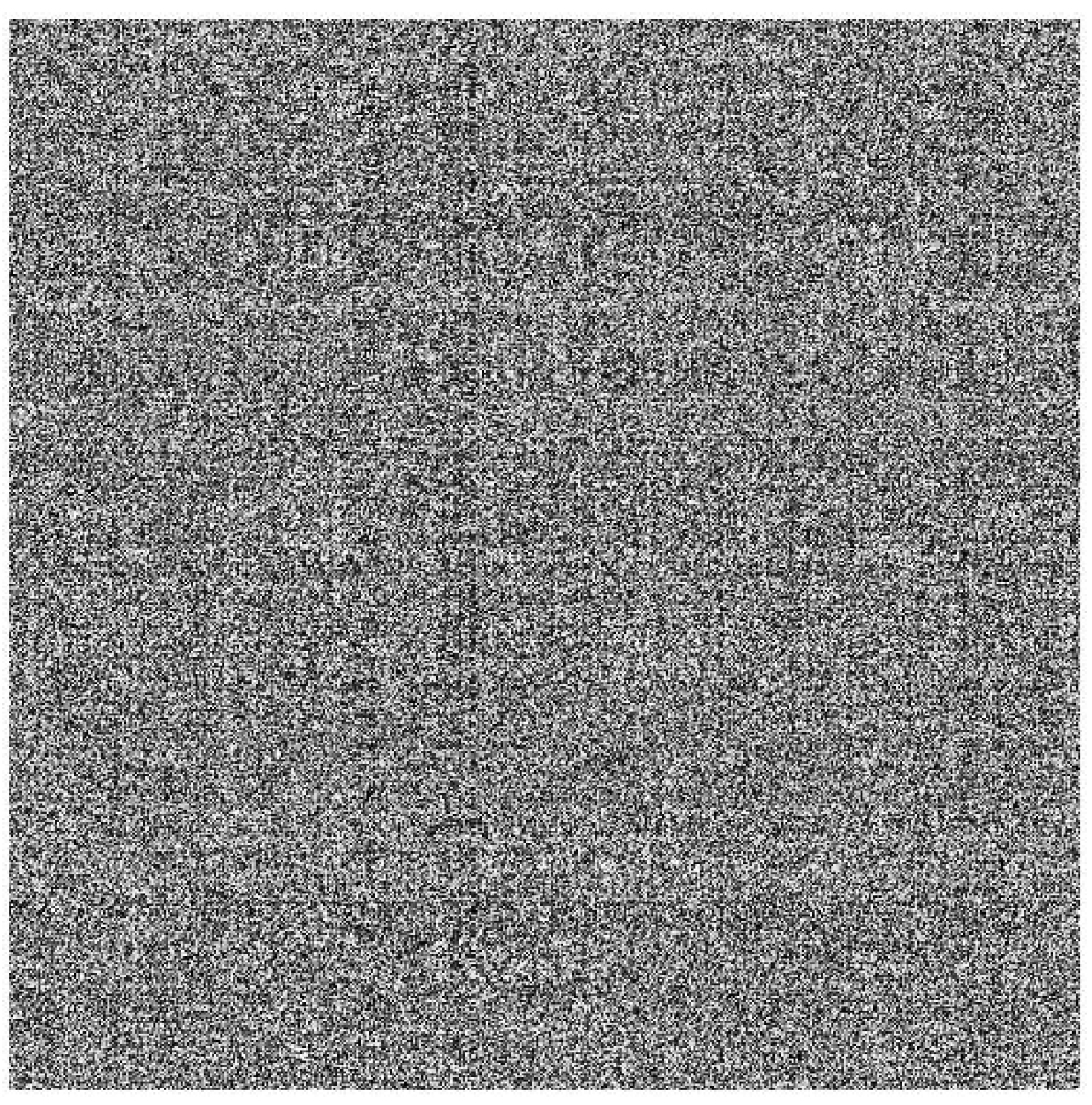
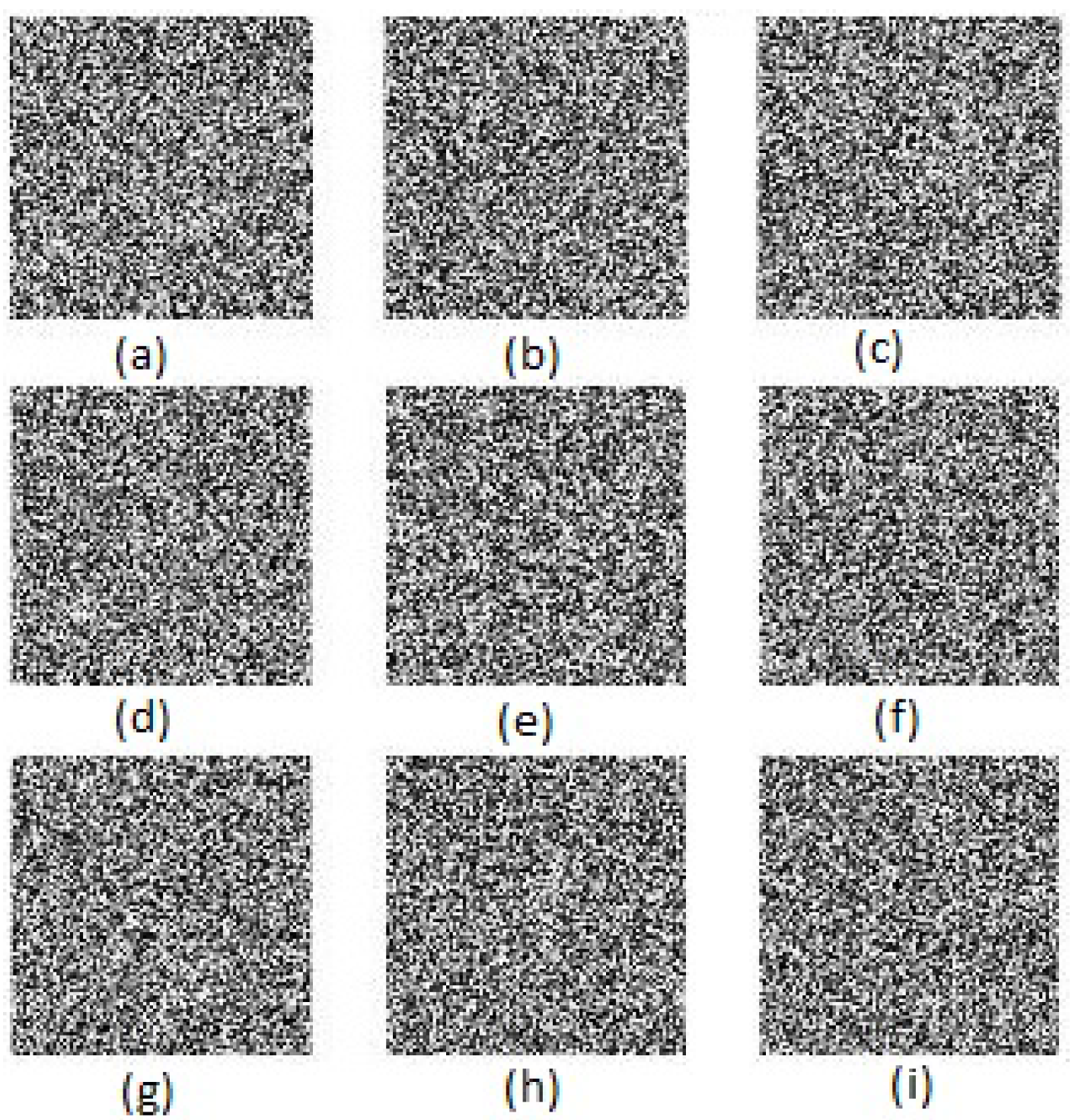
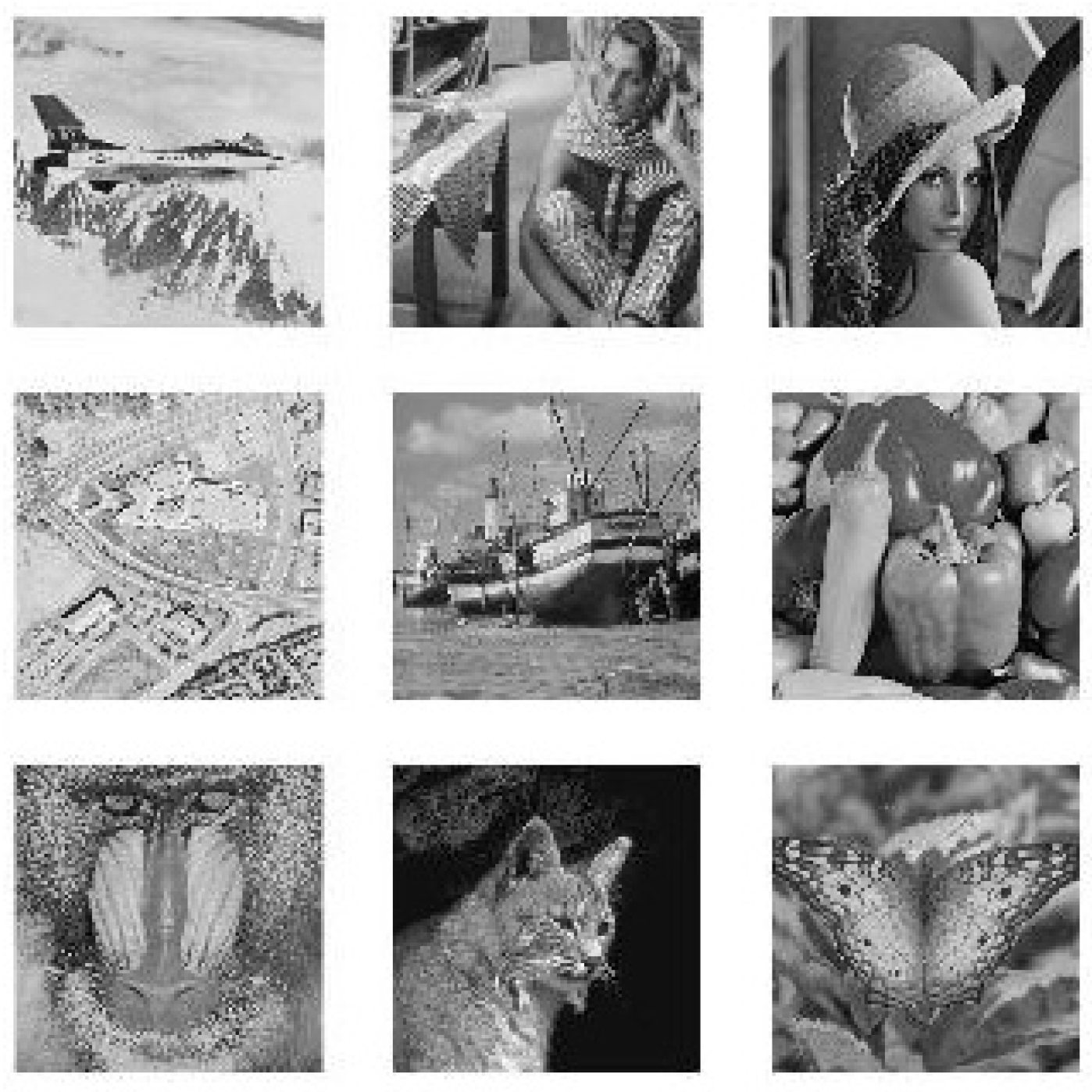
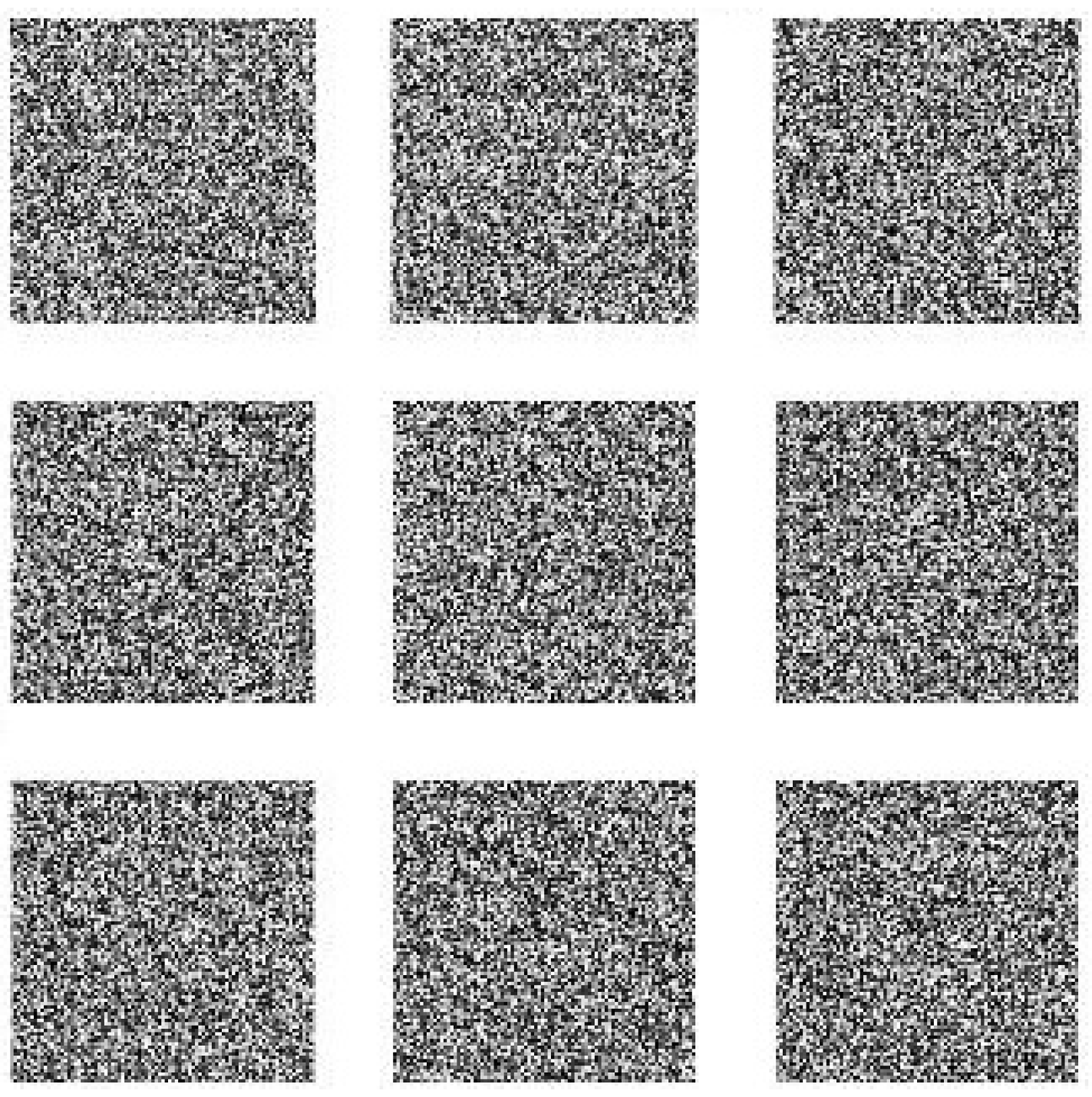
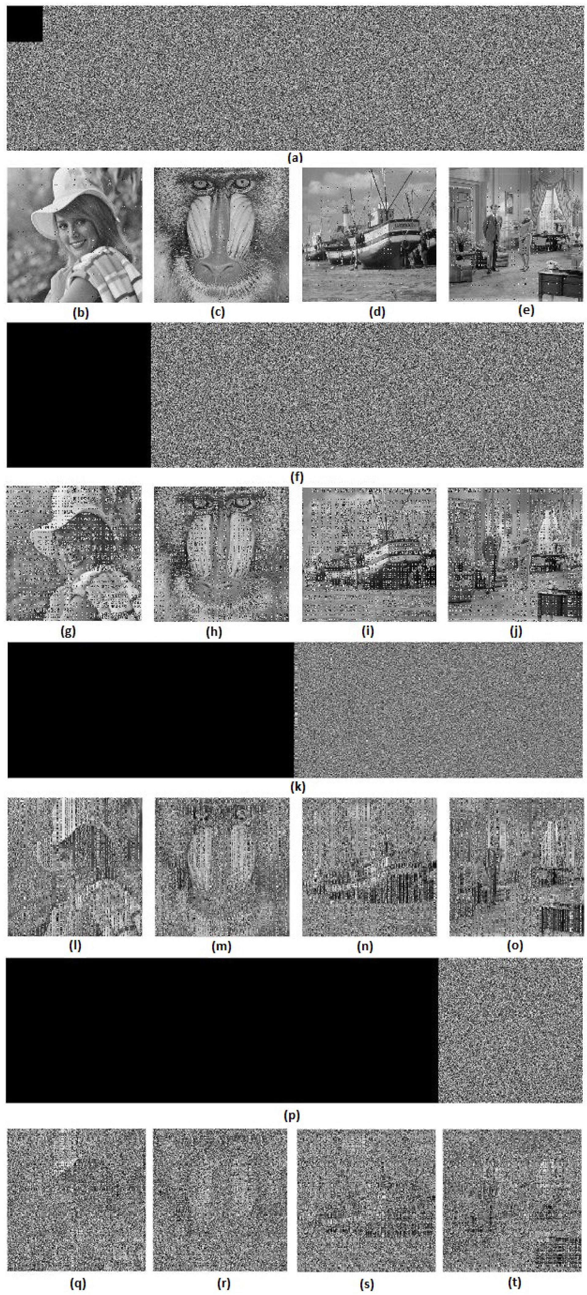
To show the efficiency and robustness of the proposed algorithm, nine () original gray images of a size are shown in Figure 6. Let be the initial values and be the parameters of the logistic map for shuffling the PIES. Furthermore, let and be the initial values and the parameters of the logistic map for shuffling the big scrambled image. Let and be the initial values and the control parameters of the chaotic economic map (1). All nine original gray images are combined into one big image, which is displayed in Figure 7. Figure 8, Figure 9, Figure 10, Figure 11, Figure 12 and Figure 13 show the big scrambled images that correspond to the MIES of equal sizes , , , , and , respectively. The corresponding encrypted images of MIES with size are shown in Figure 14. Furthermore, the corresponding decrypted images are displayed in Figure 15. Experiments are performed with MATLAB R2016a software to execute the proposed algorithm on a laptop with the following characteristics: 2.40 GHz Intel Core i7-4700MQ CPU and 12.0 GB RAM memory.
The performance of the presented multiple-image encryption algorithm is investigated in detail as follows.
6.1. Analysis of the Key Space
A large key space is required to make the brute-force attack infeasible [10]. In the proposed algorithm, the key space was selected as follows. In the logistic map, were selected to shuffle rows and columns. and k were selected for the chaotic economic map (1). Then, the key space size was if the computer precision were . Table 1 shows that the key spaces in [10,20,22] were less than the presented key space. Therefore, it was large enough to make the brute-force attack infeasible.
6.2. Analysis of the Key Sensitivity
An excellent multiple-image encryption algorithm should be very sensitive to modifying any key of the encryption and the decryption processes. Making a small modification to the key of the encryption, the output encrypted image (the second one) should be absolutely unlike the first encrypted image. Furthermore, if the encryption and decryption keys have a small difference, then the encrypted image cannot be restored correctly [23]. The restored images of the encrypted images in Figure 14 with a small change of the secret key, say instead of , and the other parameters unchanged, are shown in Figure 16. The result shows that a small modification of the key can lead to completely different encrypted images, and the restoration of original images becomes very complicated. As the sensitivity of and k was the same as , their examples are omitted here.
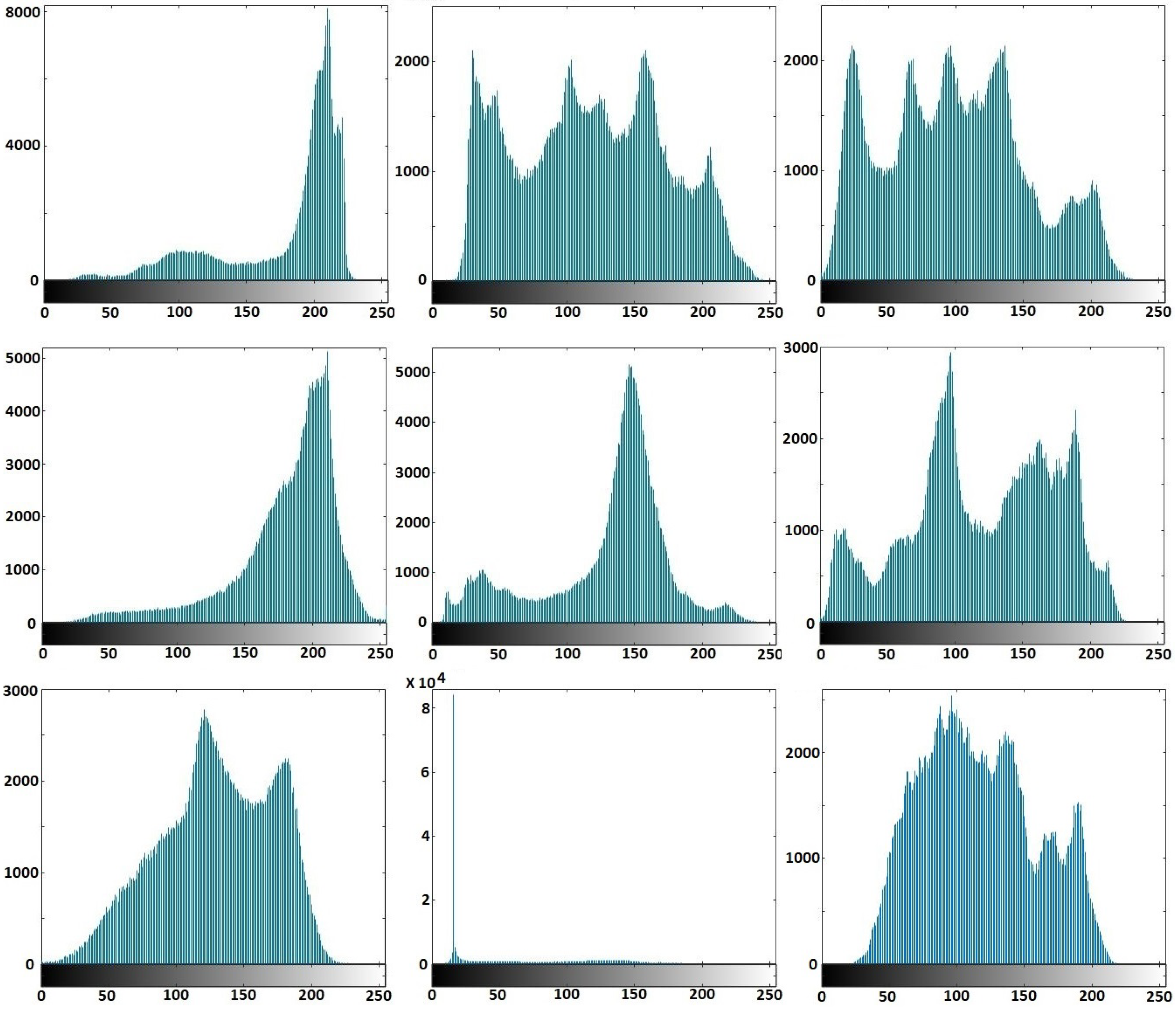
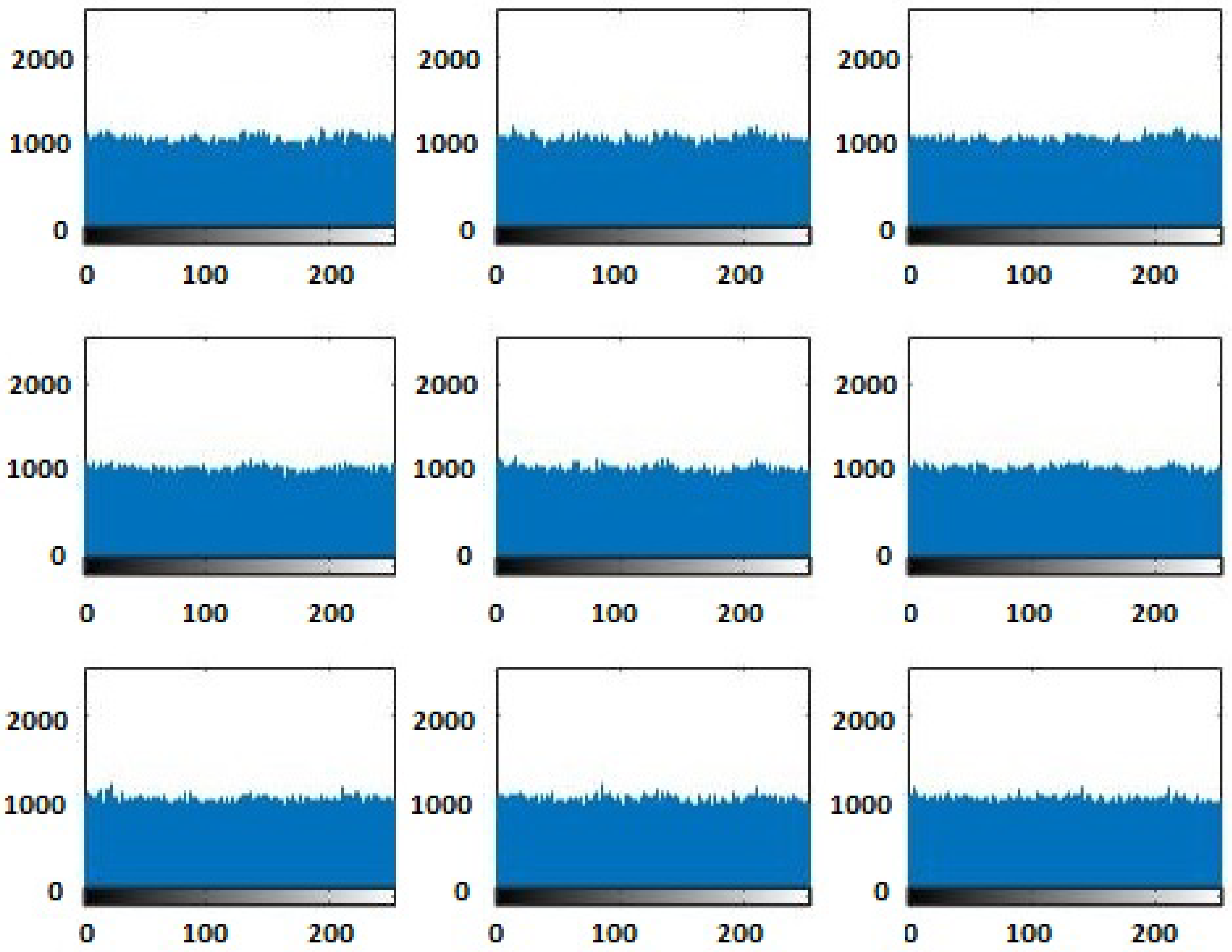
6.3. Analysis of the Histogram
The original images’ histograms are shown in Figure 17, while the corresponding encrypted images histograms are shown in Figure 18. Figure 16 and Figure 18 display that the original images had different histograms, while the corresponding encrypted images histograms had a uniform distribution approximately. Therefore, the encryption process damaged the original images’ features.
6.4. Analysis of Histogram Variance
The histogram variance of a gray image is defined by:
where and V is the pixel number vector of 256 gray levels.
This can clarify the impact of the encrypted image to some degree. In a perfect random image, all the gray levels have equal probabilities. Therefore, the histogram variance equals zero. Therefore, the histogram variance of the encrypted image via an effective encryption algorithm should tend to zero. Table 2 shows the values of the histogram variances of the encrypted images of the original images in Figure 19 via Tang’s algorithm [20], Zhang’s algorithm [10] and the proposed algorithm, respectively.
6.5. Analysis of Information Entropy
In a digital image, the information entropy can be an indicator of the pixel values’ distribution. For a perfect random image, , where is the i-th gray level of the image and is the probability of . Furthermore, it has information entropy . Now, the information entropy is computed by [24]:
Table 3 lists the values of information entropy for the encrypted images in Figure 14. The information entropy of the encrypted images of the proposed algorithm is better than the information entropy of the encrypted images of the multiple-image encryption algorithm in [10]. Therefore, the efficiency and security of the proposed algorithm is clear.
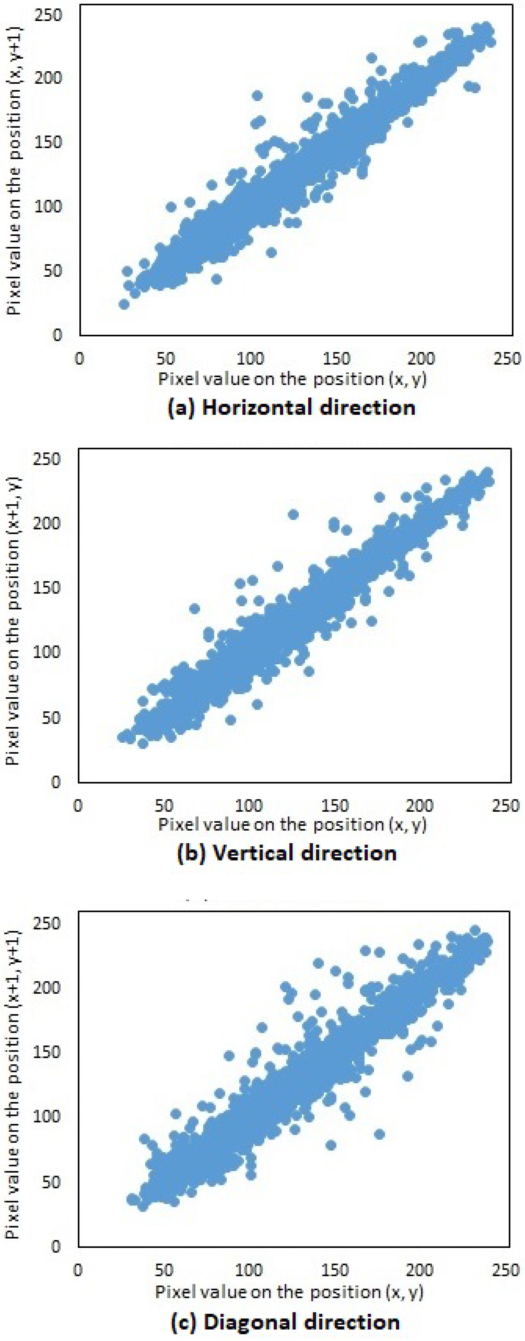
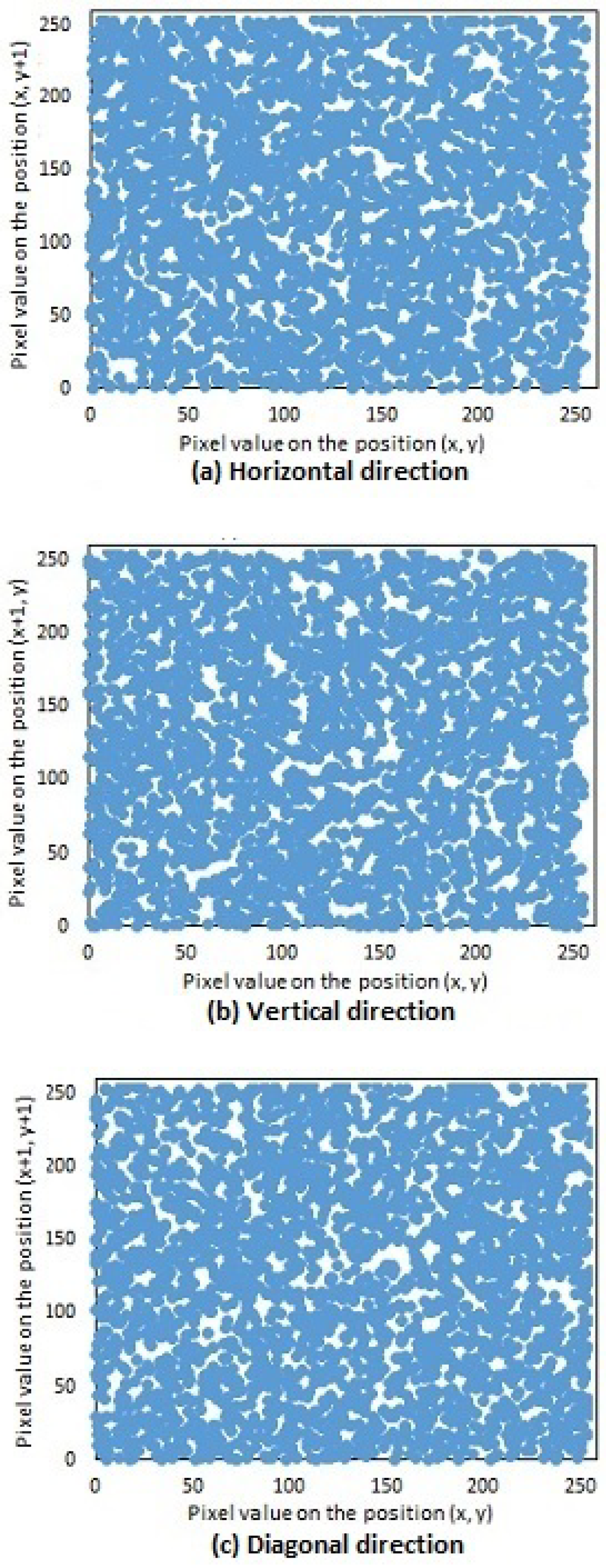
6.6. Analysis of the Correlation Coefficients
In the image encryption, the correlation coefficient was used to measure the correlation between two neighboring pixels, horizontally, vertically and diagonally neighboring. It is evaluated by [25]:
where:
and
Three thousand pairs of pixels were selected randomly in all three directions from the two images (original and encrypted); see Figure 19a and Figure 21a, respectively. Then, the correlation coefficients of the two neighboring pixels were computed using Equation (4). The neighboring pixel correlation of Figure 19a and Figure 20a are plotted in Figure 21 and Figure 22. Their correlation coefficients are illustrated in Table 4 and Table 5. The original images’ correlation coefficients were approximately equal to one, while the corresponding ones of encrypted images were approximately equal to zero. The results conclude that the proposed algorithm can conserve the image information.
6.7. Analysis of Differential Attack
In the differential attack, the encryption algorithm was used to encrypt the original image before and after modification, then the two encrypted images were compared to discover the link between them [26]. Therefore, a good image encryption algorithm should be the desired property to spread the effect of a minor change in the original image of as much an encrypted image as possible. Number of pixels change rate (NPCR) and unified averaged changed intensity (UACI) are famous measurements, which were used to measure the resistance of the image encryption algorithm for differential attacks. The NPCR and UACI are defined as follows,
where:
M and N are the width and height of the original and the encrypted images; and are the encrypted images before and after one pixel changed from the original image. For example, a pixel position was selected randomly, and it has the value 159 in Figure 19a. The pixel value was modified to 244 to examine the ability to combat the differential attacks. Table 6 lists the results of Figure 19a–d. The results show that a small modification in the plain image will result in a big modification in the cipher image. Therefore, the proposed algorithm can face differential attacks.
6.8. Chosen/Known Plaintext Attack Analysis
Attackers have used two famous attacks called chosen-plaintext attack and known-plaintext attack for attacking any cryptosystem. The secret keys are not only dependent on the given initial values and system parameters, but also on the plain images. Therefore, when the plain images are changed, the secret keys will be changed in the encryption process. Therefore, attackers cannot take important information by encrypting some predesigned special images. Therefore, the proposed algorithm robustly resisted both attacks.
6.9. Noise Attack Analysis
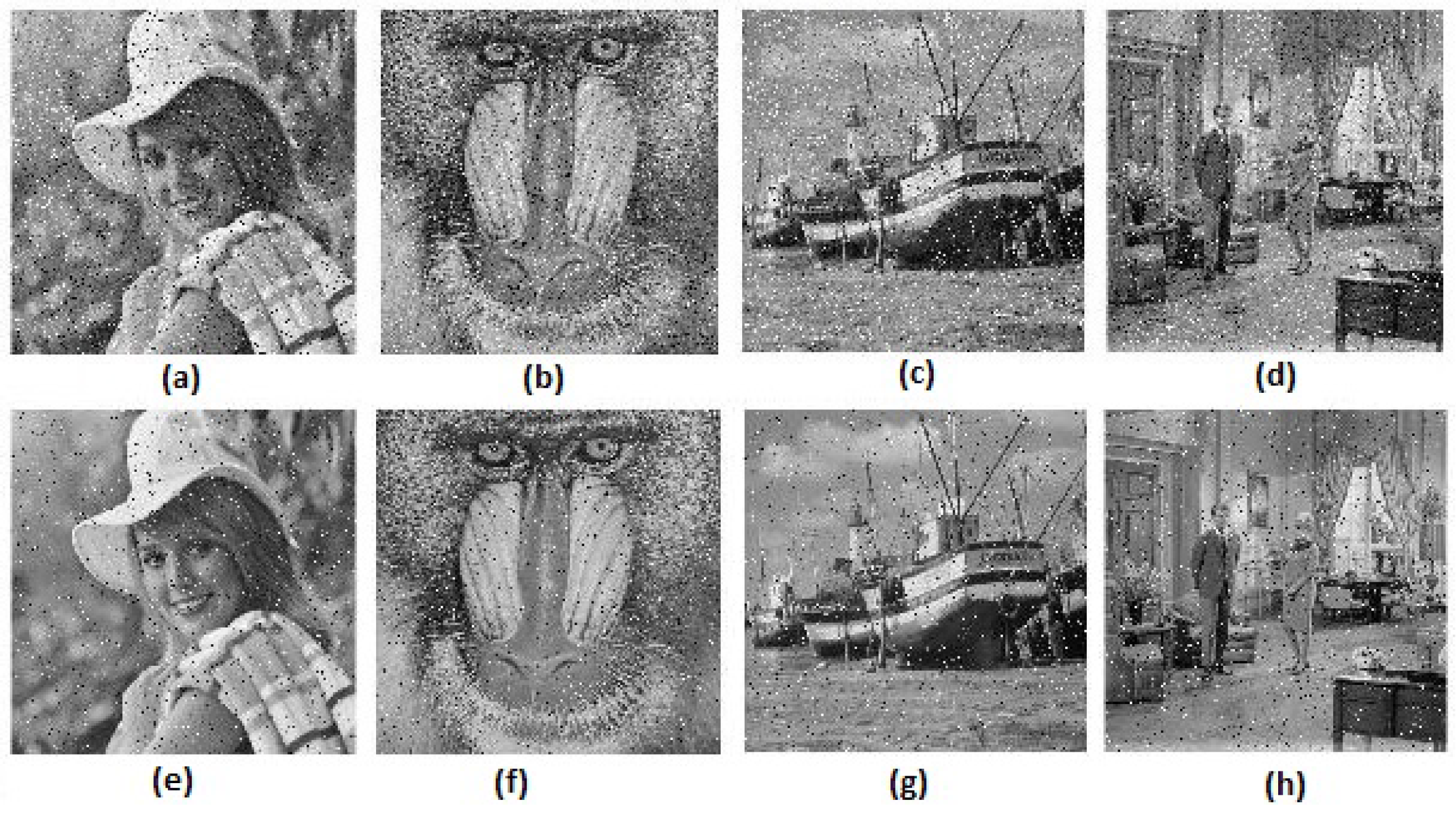
The encrypted images in Figure 20 are distorted by adding Gaussian noise with mean = 0 and variance = and salt and pepper noise with density = 0.05. The corresponding decrypted images are displayed in Figure 23. Moreover, Table 7 shows the mean squared error (MSE) and the peak signal-to-noise ratio (PSNR) between input images and decrypted images based on the proposed algorithm. Based on Table 7, we can conclude that the proposed algorithm had the highest resisting ability to salt and pepper noise since the PSNR was more than 65 (dB).
6.10. Analysis of Occlusion Attack
The current section is assigned to the analyses of occluded data decryption. Data that are occluded are hidden or ignored data inside the process. Firstly, and sized data occlusions of the horizontally concatenated encrypted image were performed. Secondly, the decrypted image of each one was analyzed. Figure 24 shows the results of the occlusion attack. Based on Figure 24, the decrypted images of sized occluded encrypted images were disfigured, but discernible by the human eye, while decrypted images of sized occluded encrypted images were not restored. Hence, the proposed algorithm could resist up to a () occlusion attack.
7. Comparison with Other Algorithms
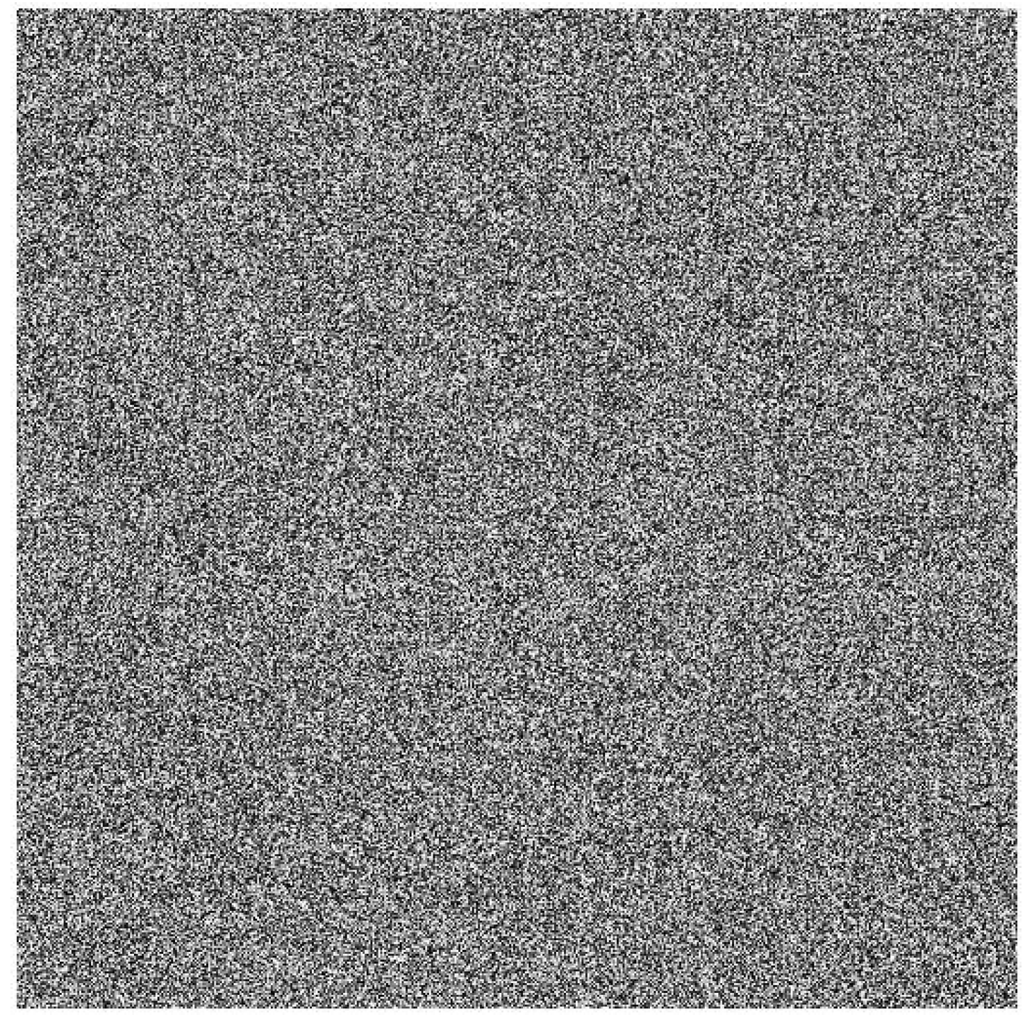
A comparison between Tang’s algorithm [20] and Zhang’s algorithm was performed in [10]. The result of the comparison concluded that Zhang’s algorithm was faster than Tang’s algorithm. Therefore, a comparison between Zhang’s algorithm and the proposed algorithm is presented. The same four original gray images are chosen as input images and are displayed in Figure 19. Furthermore, the size of MIES = is selected. The encrypted images of the proposed algorithm and Zhang’s algorithm are shown in Figure 20 and Figure 25, respectively. The computational times of both algorithms are listed in Table 8. Although the time of Zhang’s algorithm is less than the proposed algorithm, the encrypted images’ histograms of the proposed algorithm are uniformly distributed, and the encrypted images histograms of Zhang’s algorithm are not uniformly distributed (see Figure 13 in [10]). Therefore, the experimental results conclude that the proposed algorithm is efficient. The security of Zhang’s algorithm is a little weaker than the proposed algorithm since the key space size of the proposed algorithm is larger than Zhang’s algorithm and two additional shuffling operations are added to the proposed algorithm, one for PIES and one for the big scrambled image.
8. Conclusions
The current paper has proposed a new multiple-image encryption algorithm using combination of MIES and a two-dimensional chaotic economic map. The key space size of the proposed algorithm is . Therefore, it gives priority to the proposed algorithm to resist against brute-force attack. The experimental results have demonstrated that the proposed algorithm produced encrypted images that have histograms with uniform distributions. In addition, the proposed algorithm has demonstrated that the encrypted images have information entropies close to eight. It robustly resists chosen/known plaintext attacks, has the highest resisting ability to salt and pepper noise and can resist up to a () occlusion attack. Comparison experiments with Zhang’s algorithm were performed. Furthermore, the analyses of the algorithm conclude that the proposed algorithm is secure and efficient. It can be applied in several fields like weather forecasting, military, engineering, medicine, science and personal affairs. In this paper, the proposed idea was simulated on grayscale images, which had the same size. In the future, the proposed idea will applied on grayscale images with different sizes.
Funding
This research received no external funding.
Acknowledgments
I deeply thank Shehzad Ahmed for his contribution in editing and proof reading the paper.
Conflicts of Interest
The author declares no conflict of interest.
References
- Askar, S.S.; Karawia, A.A.; Alshamrani, A. Image encryption algorithm based on chaotic economic model. Math. Probl. Eng. 2015, 2015, 341729. [Google Scholar] [CrossRef]
- Askar, S.S.; Karawia, A.A.; Alammar, F.S. Cryptographic algorithm based on pixel shuffling and dynamical chaotic economic map. IET Image Process. 2018, 12, 158–167. [Google Scholar] [CrossRef]
- Cao, Y.; Fu, C. An image encryption scheme based on high dimension chaos system. In Proceedings of the 2008 International Conference on Intelligent Computation Technology and Automation, Changsha, China, 20–22 October 2008; pp. 104–108. [Google Scholar]
- Jeyamala, J.; GrpiGranesh, S.; Raman, S. An image encryption scheme based on one time pads-a chaotic approach. In Proceedings of the 2010 Second International conference on Computing, Communication and Networking Technologies, Karur, India, 29–31 July 2010; pp. 1–6. [Google Scholar]
- Sivakumar, T.; Venkatesan, R. Image encryption based on pixel shuffling and random key stream. Int. J. Comput. Inf. Technol. 2014, 3, 1468–1476. [Google Scholar]
- Zhang, J.; Fang, D.; Ren, H. Image encryption algorithm based on DNA encoding and chaotic maps. Math. Probl. Eng. 2014, 2014, 917147. [Google Scholar] [CrossRef]
- Vaferi, E.; Sabbaghi-Nadooshan, R. A new encryption algorithm for color images based on total chaotic shuffling scheme. Opt.-Int. J. Light Electron Opt. 2015, 126, 2474–2480. [Google Scholar] [CrossRef]
- Elsheh, E.; Hamza, A. Secret sharing approaches for 3D object encryption. Expert Syst. Appl. 2011, 38, 13906–13911. [Google Scholar] [CrossRef]
- Wang, J.; Ding, Q. Dynamic rounds chaotic block cipher based on keyword abstract extraction. Entropy 2018, 20, 693. [Google Scholar] [CrossRef]
- Zhang, X.; Wang, X. Multiple-image encryption algorithm based on mixed image element and chaos. Comput. Electr. Eng. 2017, 62, 401–413. [Google Scholar] [CrossRef]
- Xiong, Y.; Quan, C.; Tay, C.J. Multiple image encryption scheme based on pixel exchange operation and vector decomposition. Opt. Lasers Eng. 2018, 101, 113–121. [Google Scholar] [CrossRef]
- Zhang, X.; Wang, X. Multiple-image encryption algorithm based on mixed image element and permutation. Opt. Lasers Eng. 2017, 92, 6–16. [Google Scholar] [CrossRef]
- Wu, J.; Xie, Z.; Liu, Z.; Liu, W.; Zhang, Y.; Liu, S. Multiple-image encryption based on computational ghost imaging. Opt. Commun. 2016, 359, 38–43. [Google Scholar] [CrossRef]
- Liu, W.; Xie, Z.; Liu, Z.; Zhang, Y.; Liu, S. Multiple-image encryption based on optical asymmetric key cryptosystem. Opt. Commun. 2015, 335, 205–211. [Google Scholar] [CrossRef]
- Deng, P.; Diao, M.; Shan, M.; Zhong, Z.; Zhang, Y. Multiple-image encryption using spectral cropping and spatial multiplexing. Opt. Commun. 2016, 359, 234–239. [Google Scholar] [CrossRef]
- Li, X.; Meng, X.; Yang, X.; Wang, Y.; Yin, Y.; Peng, X.; He, W.; Dong, G.; Chen, H. Multiple-image encryption via lifting wavelet transform and XOR operation based on compressive ghost imaging scheme. Opt. Lasers Eng. 2018, 102, 106–111. [Google Scholar] [CrossRef]
- Lin, Q.; Yin, F.; Mei, T.; Liang, H. A blind source separation-based method for multiple images encryption. Image Vis. Comput. 2008, 26, 788–798. [Google Scholar] [CrossRef]
- Wang, Q.; Guo, Q.; Zhou, J. Double image encryption based on linear blend operation and random phase encoding in fractional Fourier domain. Opt. Commun. 2012, 285, 4317–4323. [Google Scholar] [CrossRef]
- Li, C.; Li, H.; Li, F.; Wei, D.; Yang, X.; Zhang, J. Multiple-image encryption by using robust chaotic map in wavelet transform domain. Opt.-Int. J. Light Electron Opt. 2018, 171, 277–286. [Google Scholar] [CrossRef]
- Tang, Z.; Song, J.; Zhang, X.; Sun, R. Multiple-image encryption with bit-plane decomposition and chaotic maps. Opt. Lasers Eng. 2016, 80, 1–11. [Google Scholar] [CrossRef]
- Parvin, Z.; Seyedarabi, H.; Shamsi, M. Breaking an image encryption algorithm based on the new substitution stage with chaotic functions. Multimed. Tools Appl. 2016, 75, 10631–10648. [Google Scholar] [CrossRef]
- Patro, K.; Acharya, B. Secure multi–level permutation operation based multiple colour image encryption. J. Inf. Secur. Appl. 2018, 40, 111–133. [Google Scholar] [CrossRef]
- Askar, S.S. Complex dynamic properties of Cournot duopoly games with convex and log-concave demand function. Oper. Res. Lett. 2014, 42, 85–90. [Google Scholar] [CrossRef]
- Wang, W.; Tan, H.; Pang, Y.; Li, Z.; Ran, P.; Wu, J. A Novel encryption algorithm based on DWT and multichaos mapping. J. Sens. 2016, 2016, 2646205. [Google Scholar] [CrossRef]
- Liu, H.; Wang, X. Color image encryption based on one-time keys and robust chaotic maps. Comput. Math. Appl. 2010, 59, 3320–3327. [Google Scholar] [CrossRef]
- Belazi, A.; Abd El-Latif, A.; Belghith, S. A novel image encryption scheme based on substitution-permutation network and chaos. Signal Process. 2016, 128, 155–170. [Google Scholar] [CrossRef]
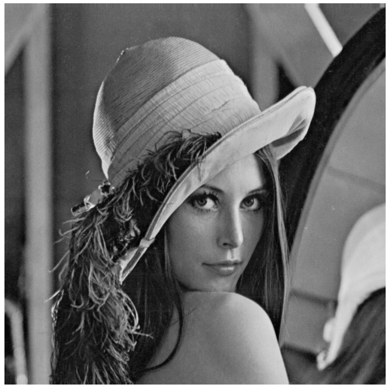
Figure 1.
Lena image with a size.

Figure 2.
Pure image elements (PIES) of the Lena image with a size.

Figure 3.
The chaotic behavior of the map (1) at and .

Figure 4.
Lyapunov exponent for the chaotic economic map (1) at and .

Figure 5.
Flowchart of multiple-image encryption.

Figure 6.
Original images.

Figure 7.
Big image.

Figure 8.
Mixed image elements (MIES) with equal size .

Figure 9.
MIES with equal size .

Figure 10.
MIES with equal size .

Figure 11.
MIES with equal size .

Figure 12.
MIES with equal size .

Figure 13.
MIES with equal size .

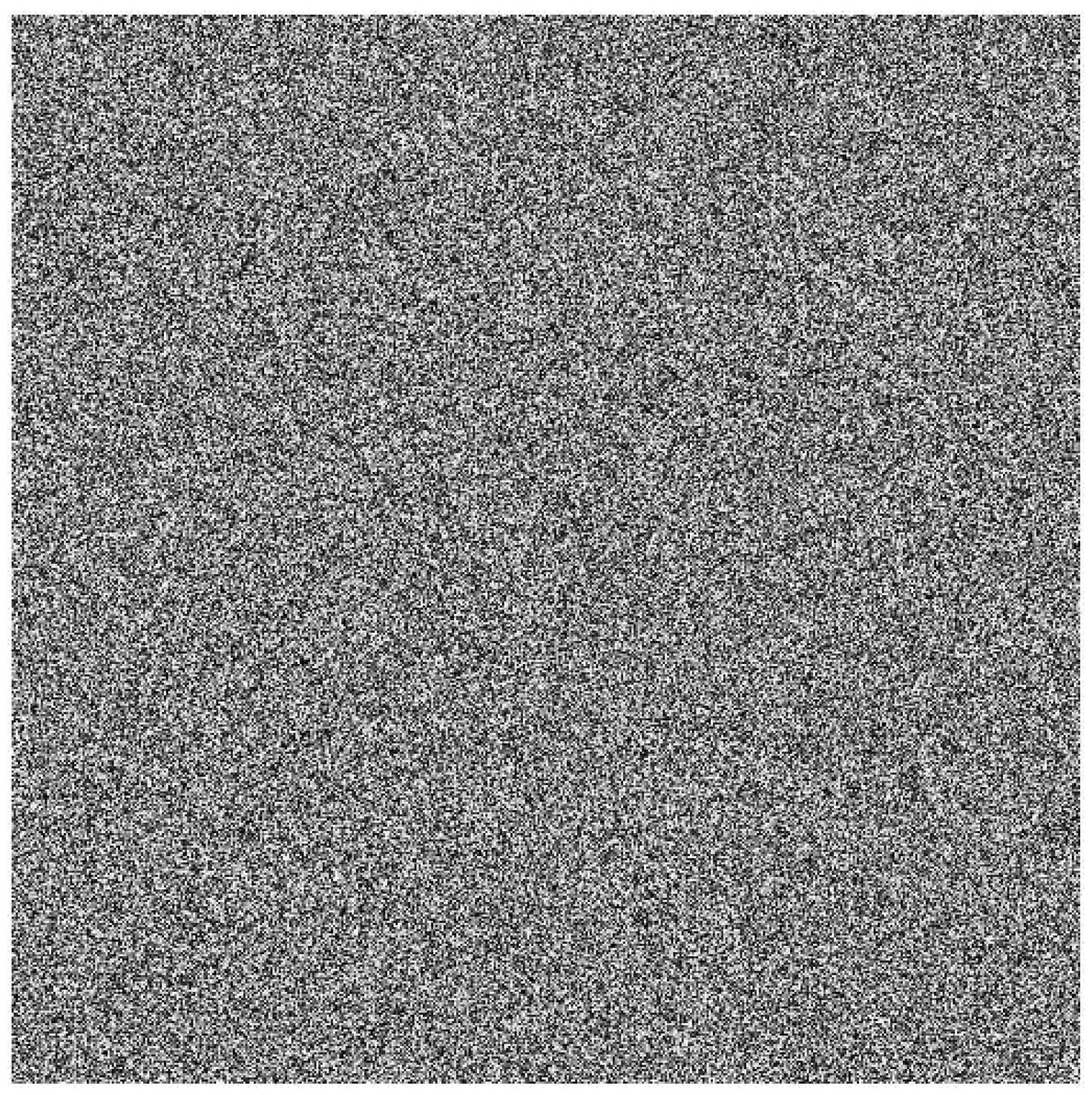
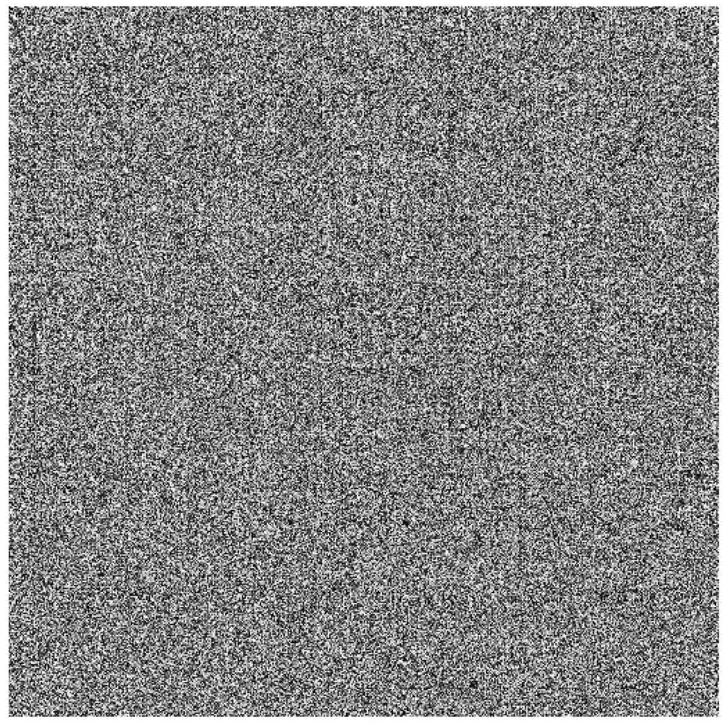
Figure 14.
Encrypted images. (a) encrypted image of airplane. (b) encrypted image of barbara. (c) encrypted image of lena. (d) encrypted image of aerial. (e) encrypted image of boat. (f) encrypted image of peppers. (g) encrypted image of baboon. (h) encrypted image of cat. (i) encrypted image of butterfly.

Figure 15.
Decrypted images.

Figure 16.
Decrypted images with the correct secret key, except , instead of .

Figure 17.
Histograms of the original images.

Figure 18.
Histograms of the encrypted images.

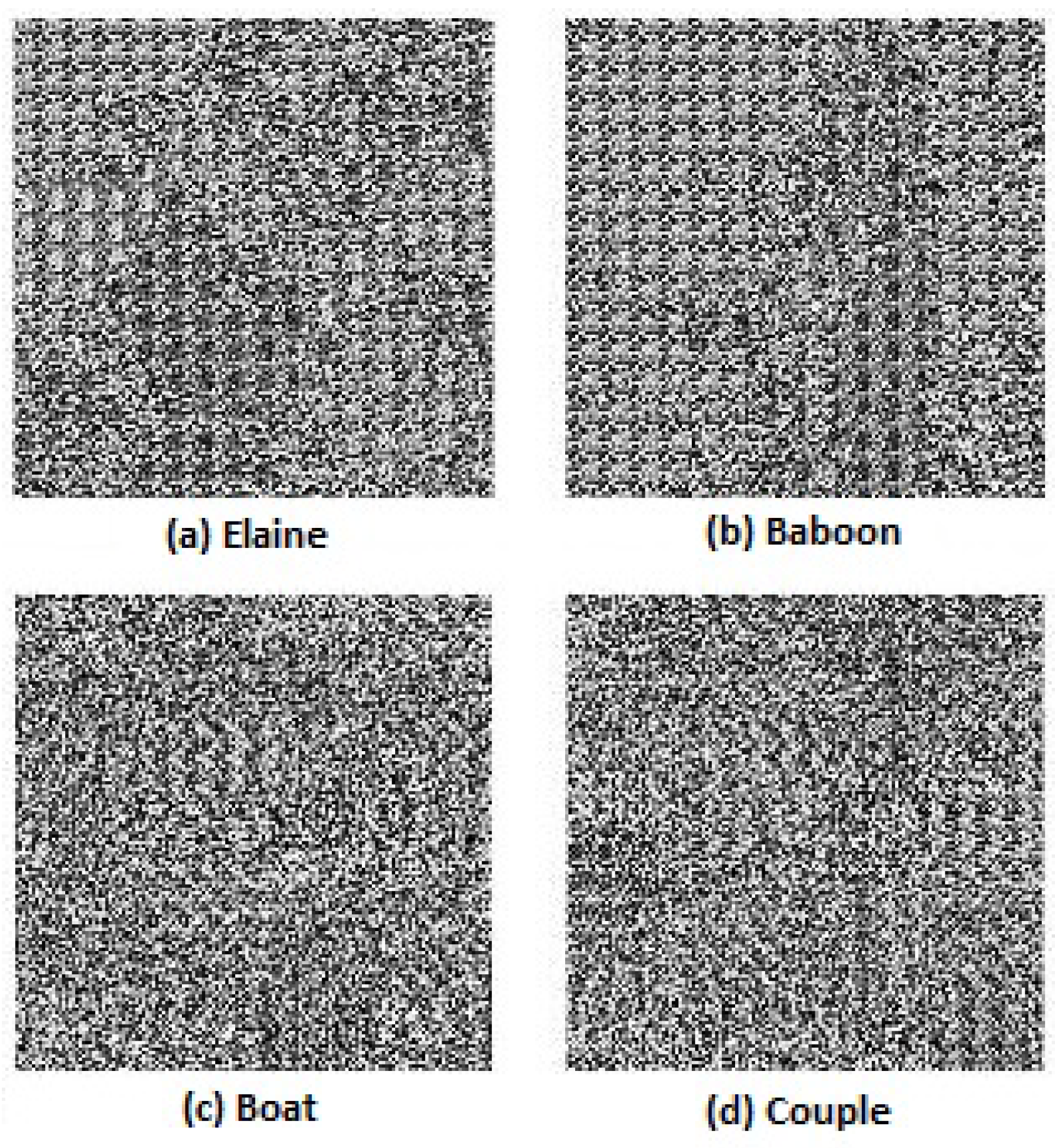
Figure 19.
Input images. (a) Elaine; (b) Baboon; (c) Boat; (d) Couple.

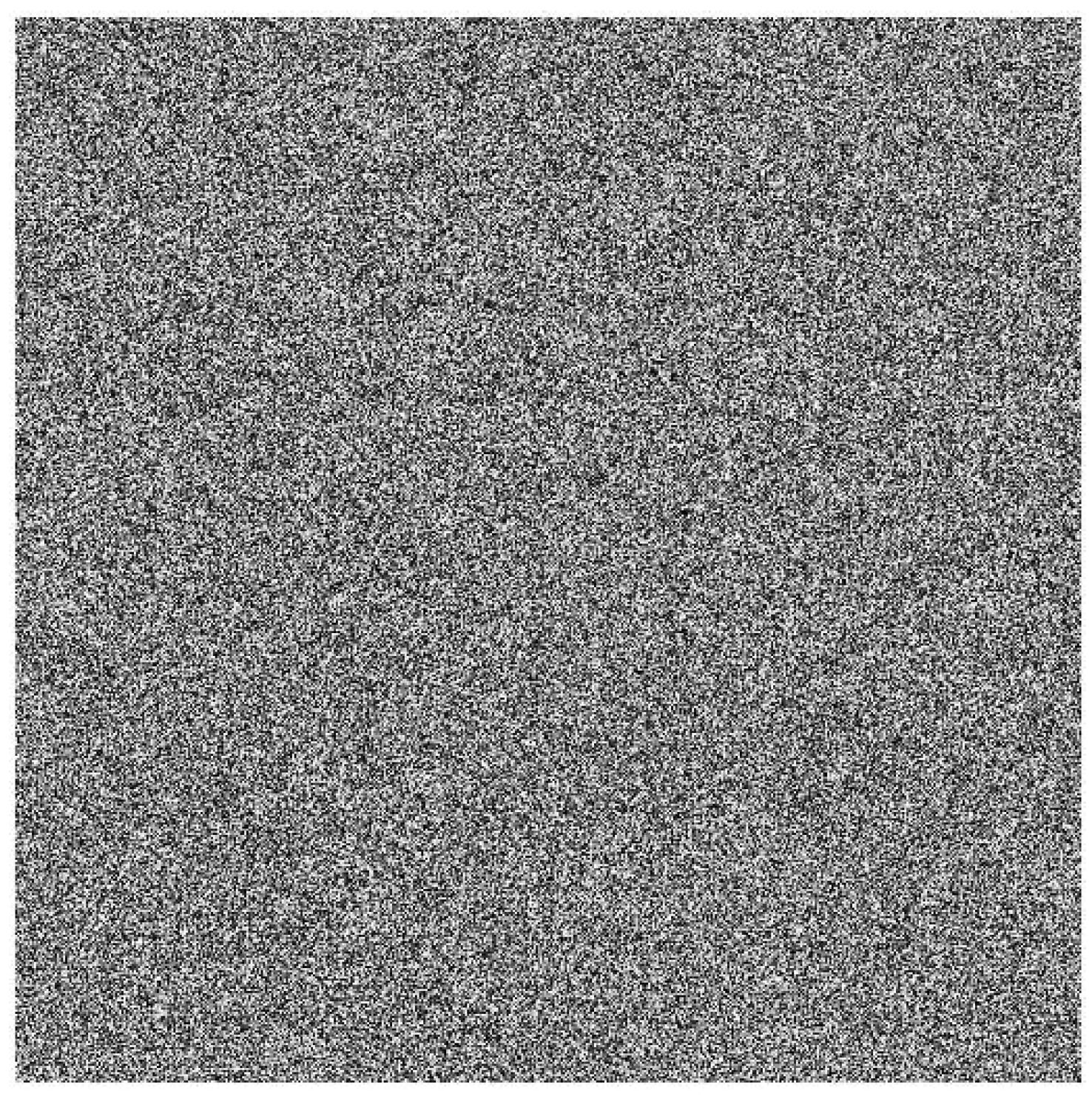
Figure 20.
Encrypted images of the proposed algorithm. (a) Elaine; (b) Baboon; (c) Boat; (d) Couple.
Figure 20.
Encrypted images of the proposed algorithm. (a) Elaine; (b) Baboon; (c) Boat; (d) Couple.

Figure 21.
Neighboring pixel correlation of Figure 19a (original image). (a) Horizontal direction; (b) Vertical direction; (c) Diagonal direction.
Figure 21.
Neighboring pixel correlation of Figure 19a (original image). (a) Horizontal direction; (b) Vertical direction; (c) Diagonal direction.

Figure 22.
Neighboring pixel correlation of Figure 20a (encrypted image). (a) Horizontal direction; (b) Vertical direction; (c) Diagonal direction.
Figure 22.
Neighboring pixel correlation of Figure 20a (encrypted image). (a) Horizontal direction; (b) Vertical direction; (c) Diagonal direction.

Figure 23.
Results of noise attack analysis: (a–d) the decrypted images after adding Gaussian noise with mean = 0 and variance = 0.001; (e–h) the decrypted images after added salt and pepper noise with density = 0.05.
Figure 23.
Results of noise attack analysis: (a–d) the decrypted images after adding Gaussian noise with mean = 0 and variance = 0.001; (e–h) the decrypted images after added salt and pepper noise with density = 0.05.

Figure 24.
Results of occlusion attack analysis: (a,f,k,p) horizontally concatenated encrypted image with a and size of occlusion, respectively; (b–e), (g–j), (l–o) and (q–t) decrypted “Elaine”, “Baboon”, “Boat” and “Couple” images, respectively, when there is a and size of occlusion in the horizontally concatenated encrypted image.

Figure 25.
Encrypted images of Zhang’s algorithm.


Table 1.
Comparison of the current key space with other key spaces in the literature.
| Algorithm | Proposed Algorithm | Ref. [10] | Ref. [20] | Ref. [22] |
|---|---|---|---|---|
| Key Space |
Table 2.
Comparison of histogram variances between three algorithms.
| Algorithm | Tang’s Algorithm [20] | Zhang’s algorithm [10] | Proposed Algorithm |
|---|---|---|---|
| Figure 19a | |||
| Figure 19b | |||
| Figure 19c | |||
| Figure 19d |
Table 3.
Information entropy for the encrypted images in Figure 14.
Table 3.
Information entropy for the encrypted images in Figure 14.
| Images | (a) | (b) | (c) |
| Entropy | 7.9984 | 7.9987 | 7.9986 |
| Images | (d) | (e) | (f) |
| Entropy | 7.9982 | 7.9986 | 7.9983 |
| Images | (g) | (h) | (i) |
| Entropy | 7.9986 | 7.9989 | 7.9986 |
Table 4.
The original images’ correlation.
| Directions | Horizontal | Vertical | Diagonal |
|---|---|---|---|
| Figure 19a | |||
| Figure 19b | |||
| Figure 19c | |||
| Figure 19d |
Table 5.
The encrypted images’ correlations.
| Directions | Horizontal | Vertical | Diagonal |
|---|---|---|---|
| Figure 20a | |||
| Figure 20b | |||
| Figure 20c | |||
| Figure 20d |
Table 6.
The values of number of pixels change rate (NPCR) and unified averaged changed intensity (UACI) for Figure 19.
Table 6.
The values of number of pixels change rate (NPCR) and unified averaged changed intensity (UACI) for Figure 19.
| Image | NPCR | UACI |
|---|---|---|
| Figure 19a | ||
| Figure 19b | ||
| Figure 19c | ||
| Figure 19d |
Table 7.
Measurements of the noise attacks of the proposed algorithm.
| Image | Noise | MSE | PSNR |
|---|---|---|---|
| Figure 23a | |||
| Figure 23b | Gaussian | ||
| Figure 23c | variance = 0.001 | ||
| Figure 23d | |||
| Figure 23a | |||
| Figure 23b | salt & pepper | ||
| Figure 23c | density = 0.05 | ||
| Figure 23d |
Table 8.
Computational time (seconds).
| Algorithm | Time |
|---|---|
| Zhang’s algorithm [10] | 2.169 |
| Proposed algorithm | 2.386 |
© 2018 by the author. Licensee MDPI, Basel, Switzerland. This article is an open access article distributed under the terms and conditions of the Creative Commons Attribution (CC BY) license (http://creativecommons.org/licenses/by/4.0/).
Share and Cite
MDPI and ACS Style
Karawia, A.A. Encryption Algorithm of Multiple-Image Using Mixed Image Elements and Two Dimensional Chaotic Economic Map. Entropy 2018, 20, 801. https://0-doi-org.brum.beds.ac.uk/10.3390/e20100801
AMA Style
Karawia AA. Encryption Algorithm of Multiple-Image Using Mixed Image Elements and Two Dimensional Chaotic Economic Map. Entropy. 2018; 20(10):801. https://0-doi-org.brum.beds.ac.uk/10.3390/e20100801
Chicago/Turabian StyleKarawia, A. A. 2018. "Encryption Algorithm of Multiple-Image Using Mixed Image Elements and Two Dimensional Chaotic Economic Map" Entropy 20, no. 10: 801. https://0-doi-org.brum.beds.ac.uk/10.3390/e20100801
Note that from the first issue of 2016, this journal uses article numbers instead of page numbers. See further details here.