Quantitative Assessment of Landslide Susceptibility Comparing Statistical Index, Index of Entropy, and Weights of Evidence in the Shangnan Area, China

Abstract
:1. Introduction
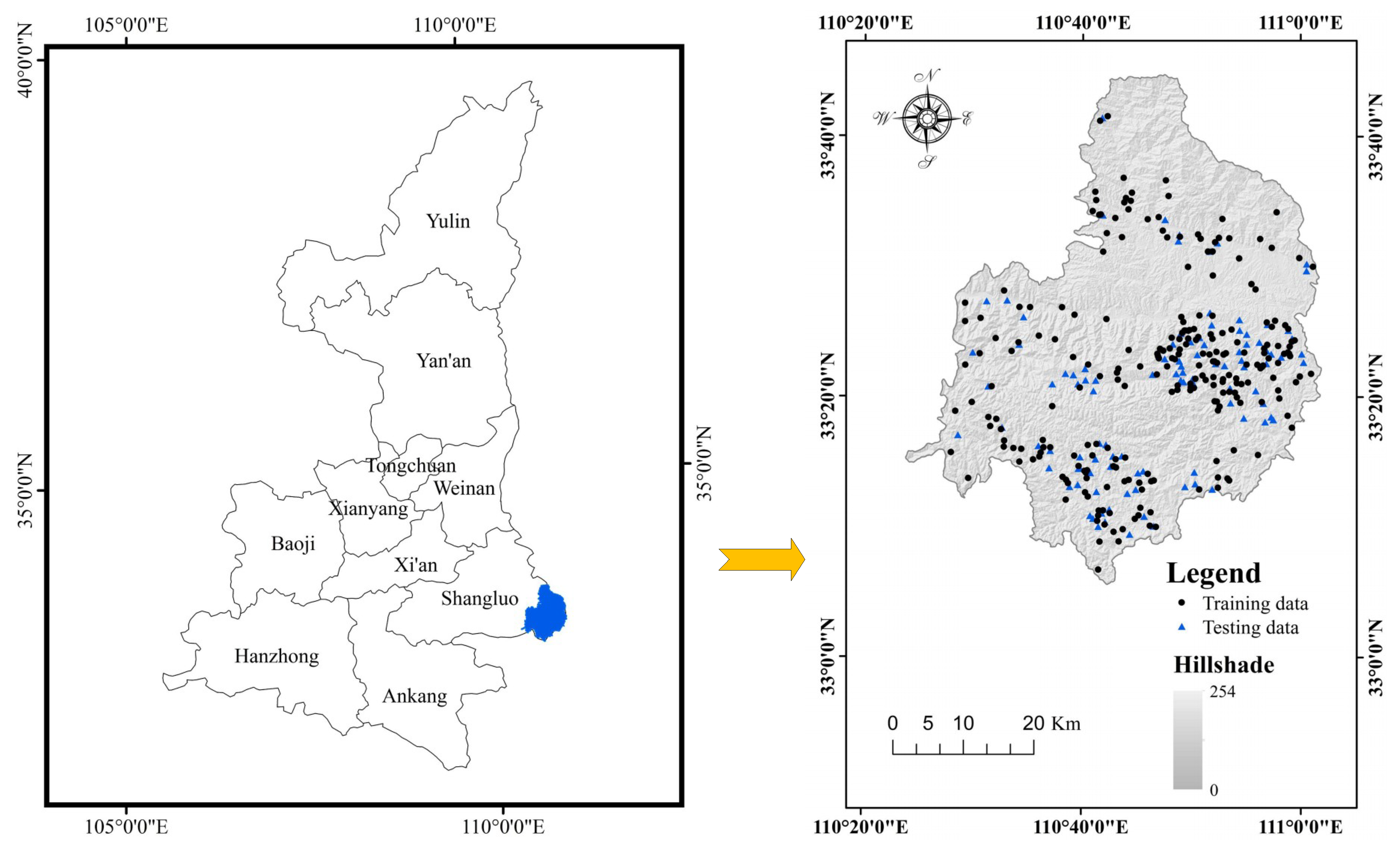
2. Study Area
3. Data
4. Modeling Approaches
4.1. Statistical Index (SI)
4.2. Index of Entropy (IOE)
4.3. Weights of Evidence (WOE)
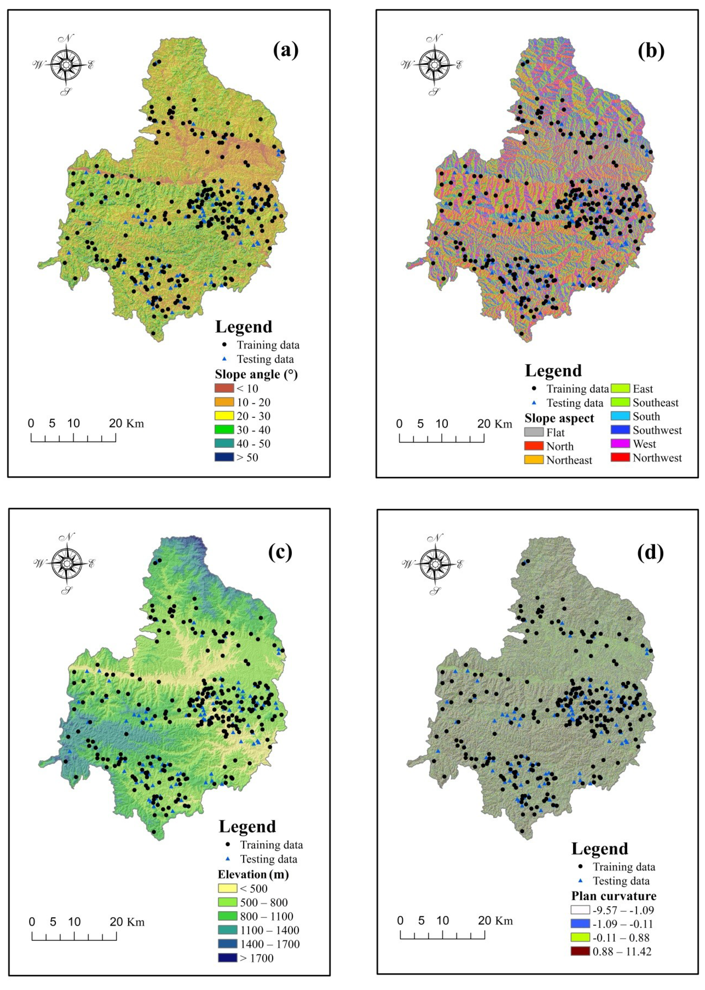
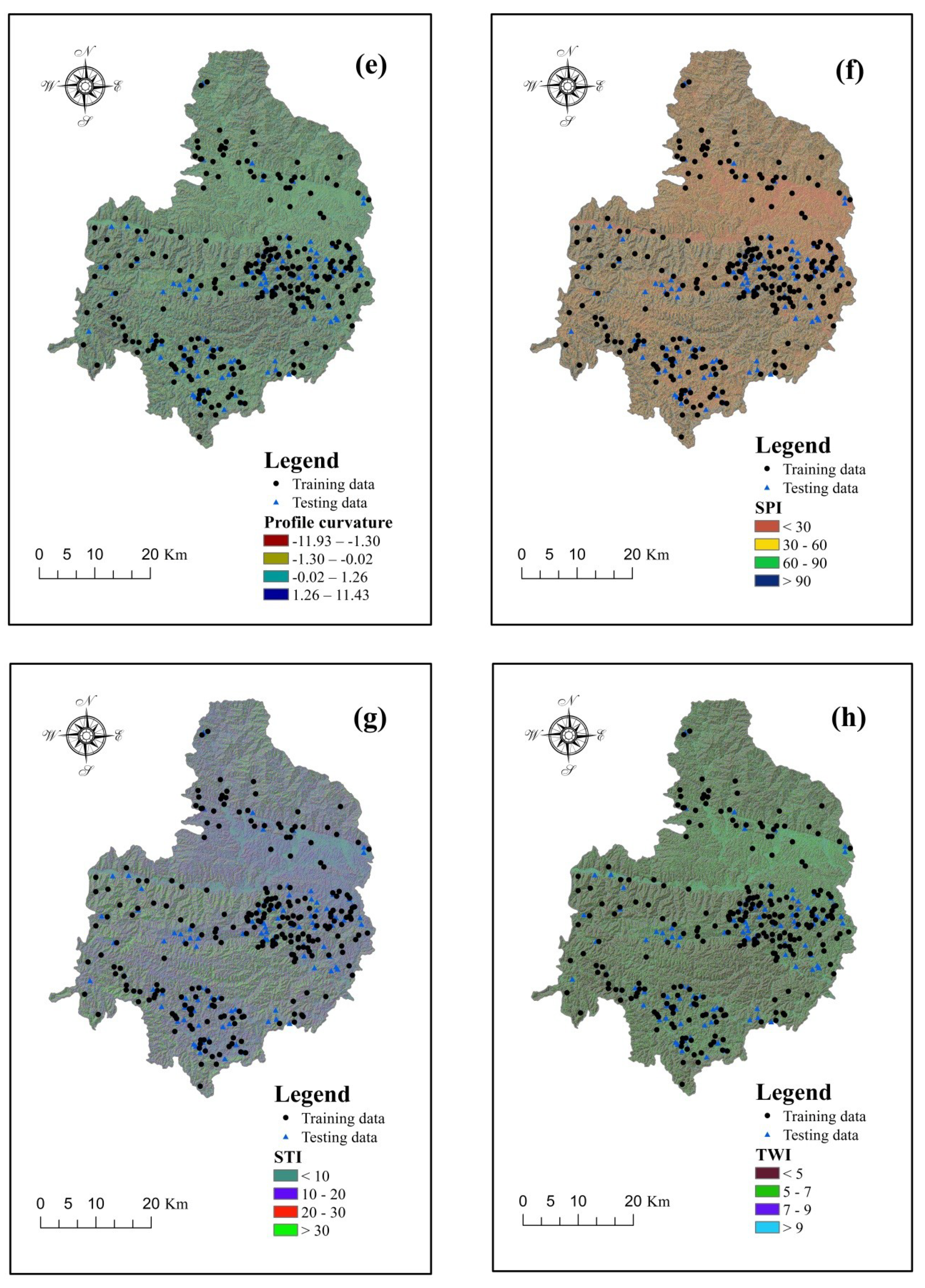
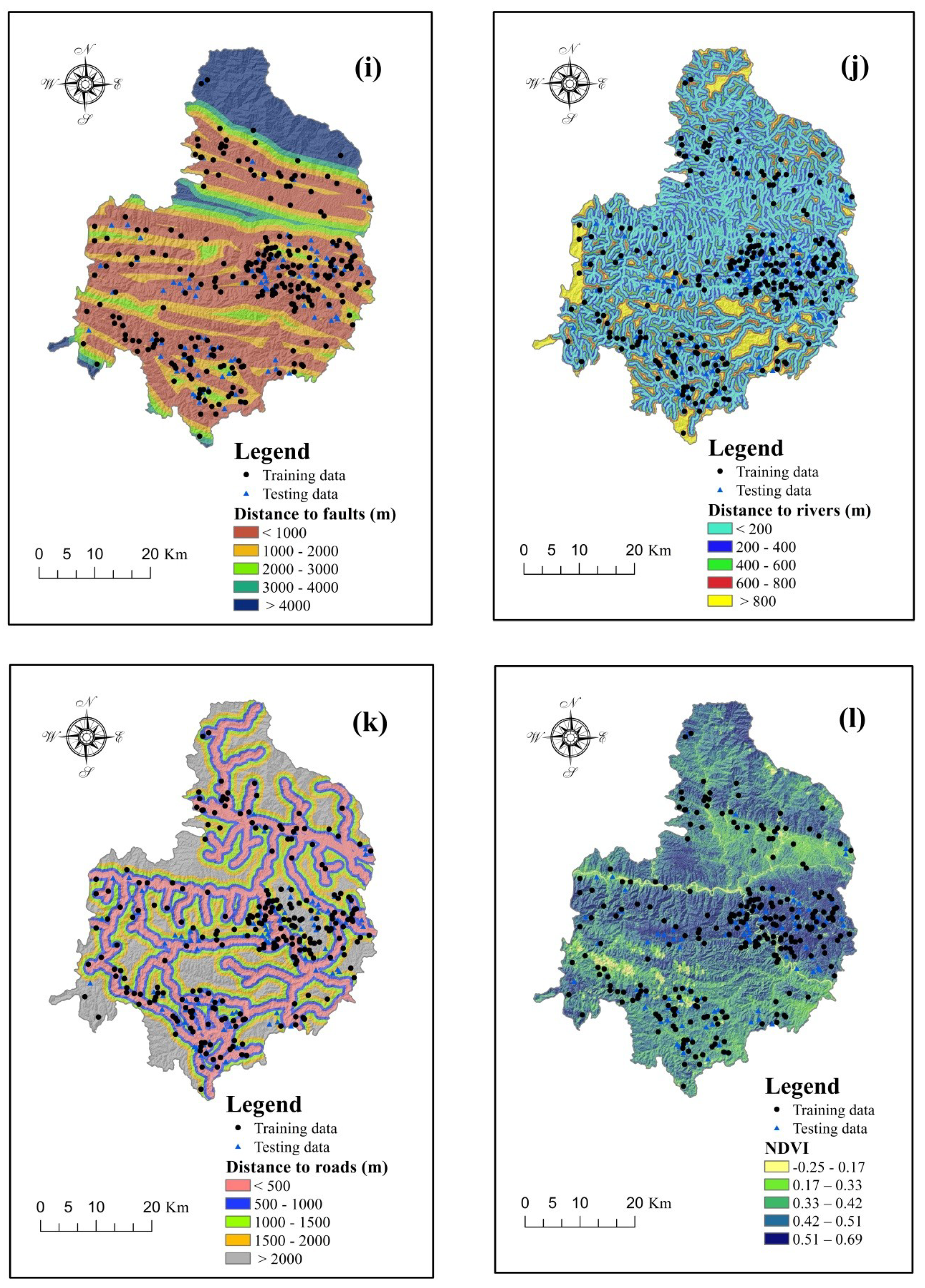
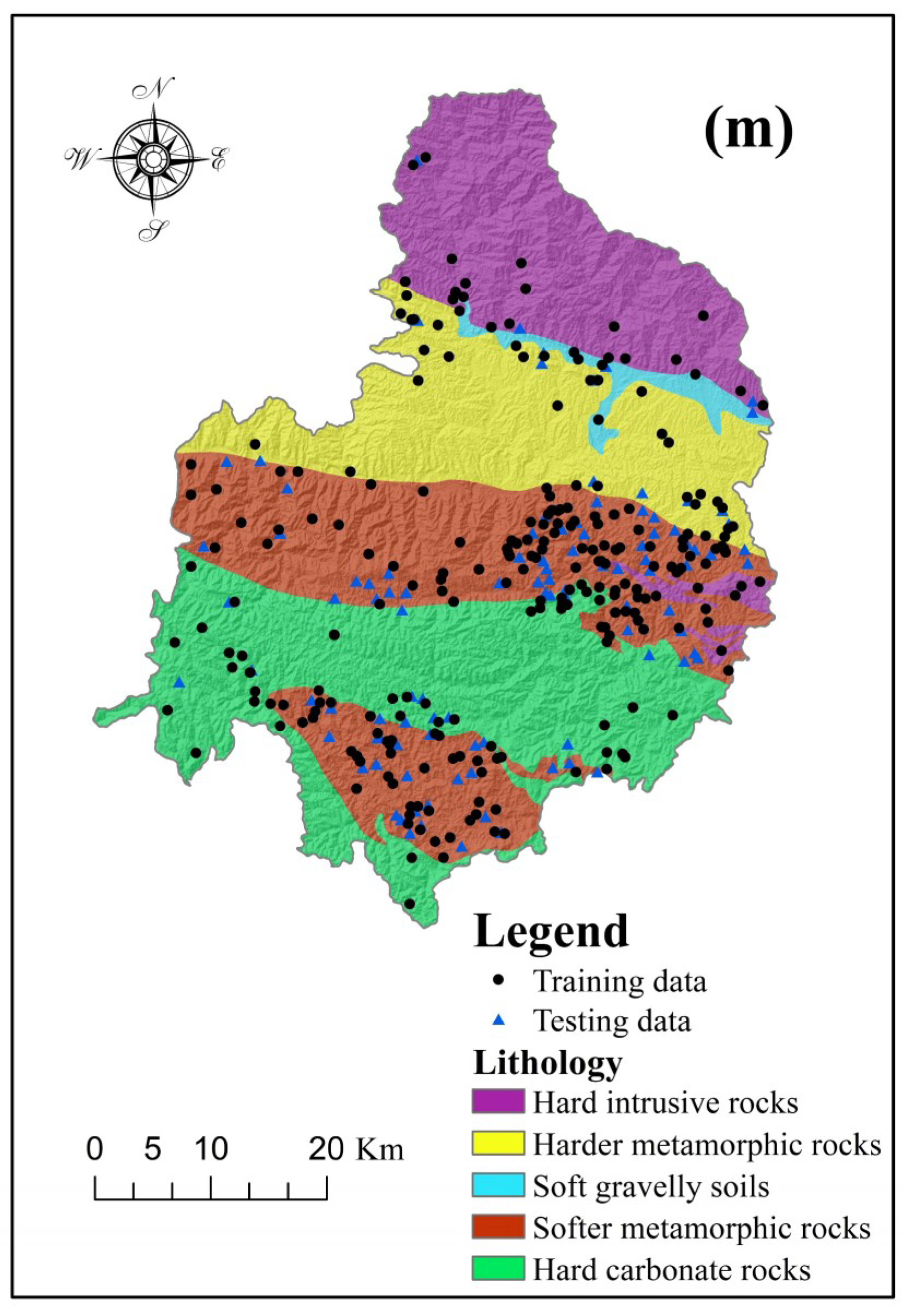
4.4. Selection of Landslide Conditioning Factors
5. Results and Discussion
5.1. Selection of Landslide Conditioning Factors
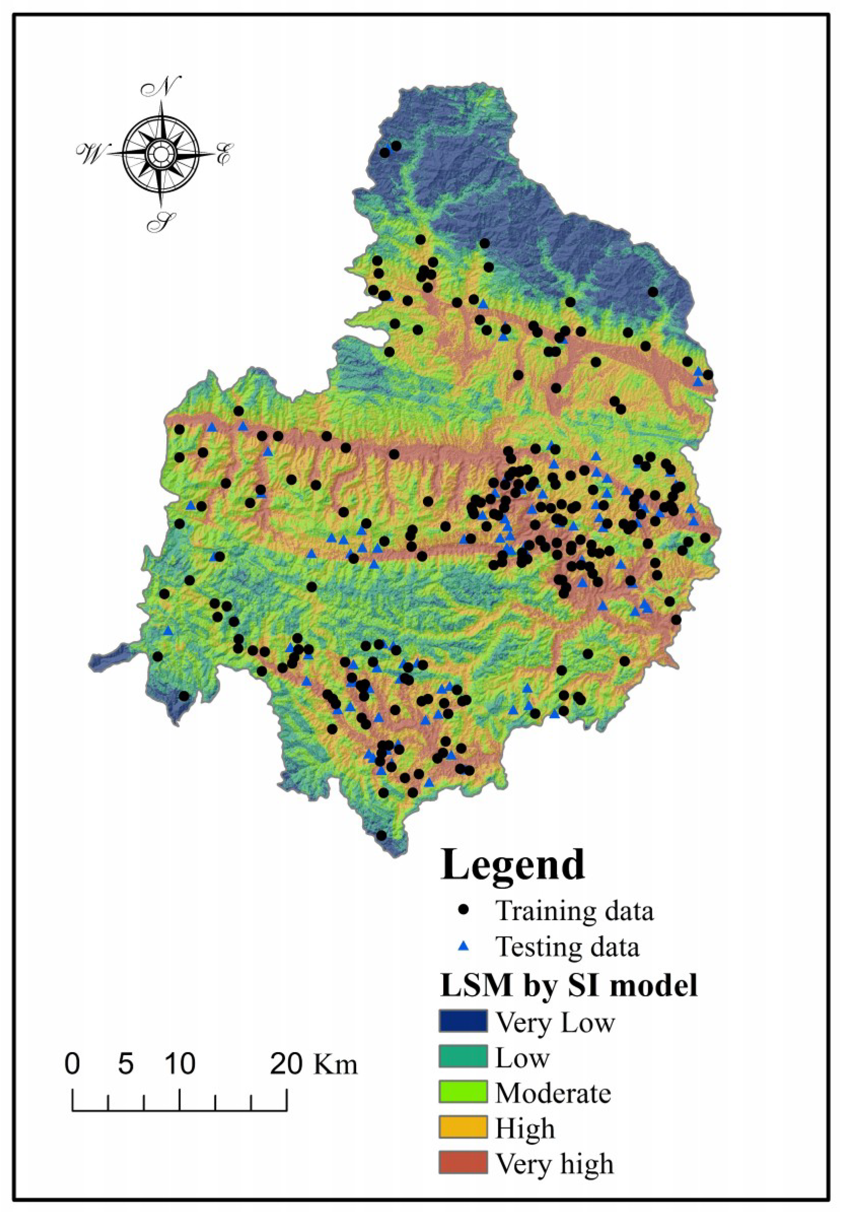
5.2. Application of the SI Model
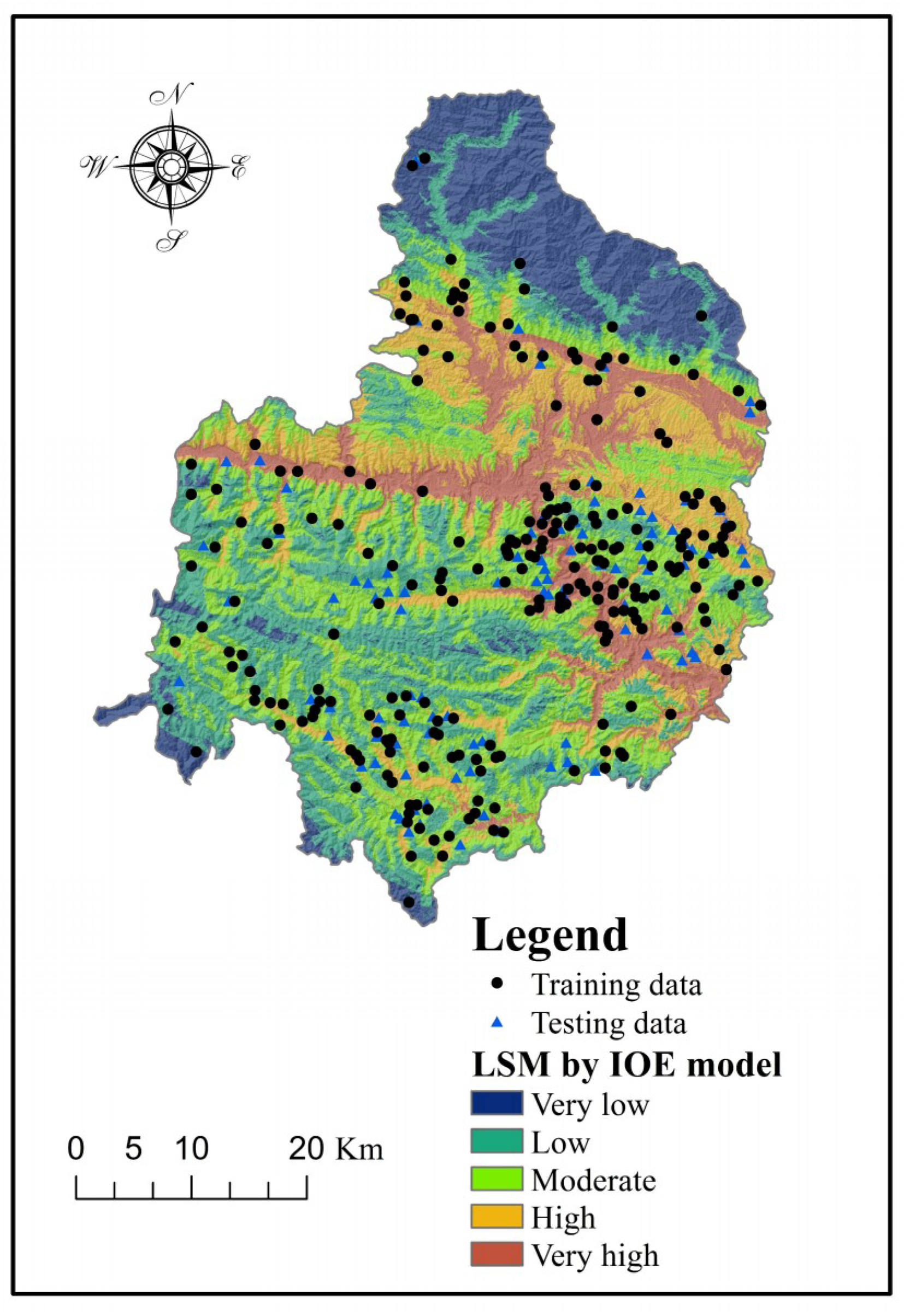
5.3. Application of the IOE Model
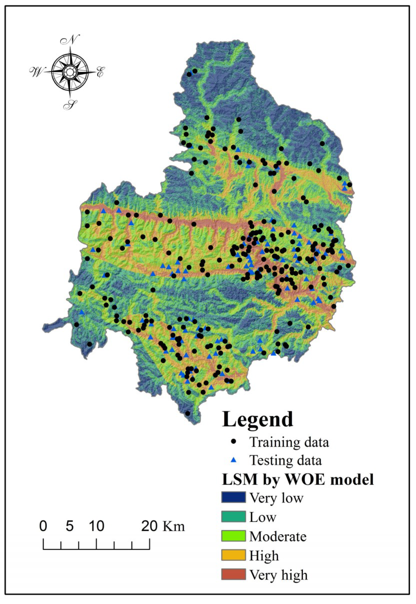
5.4. Application of the WOE Model
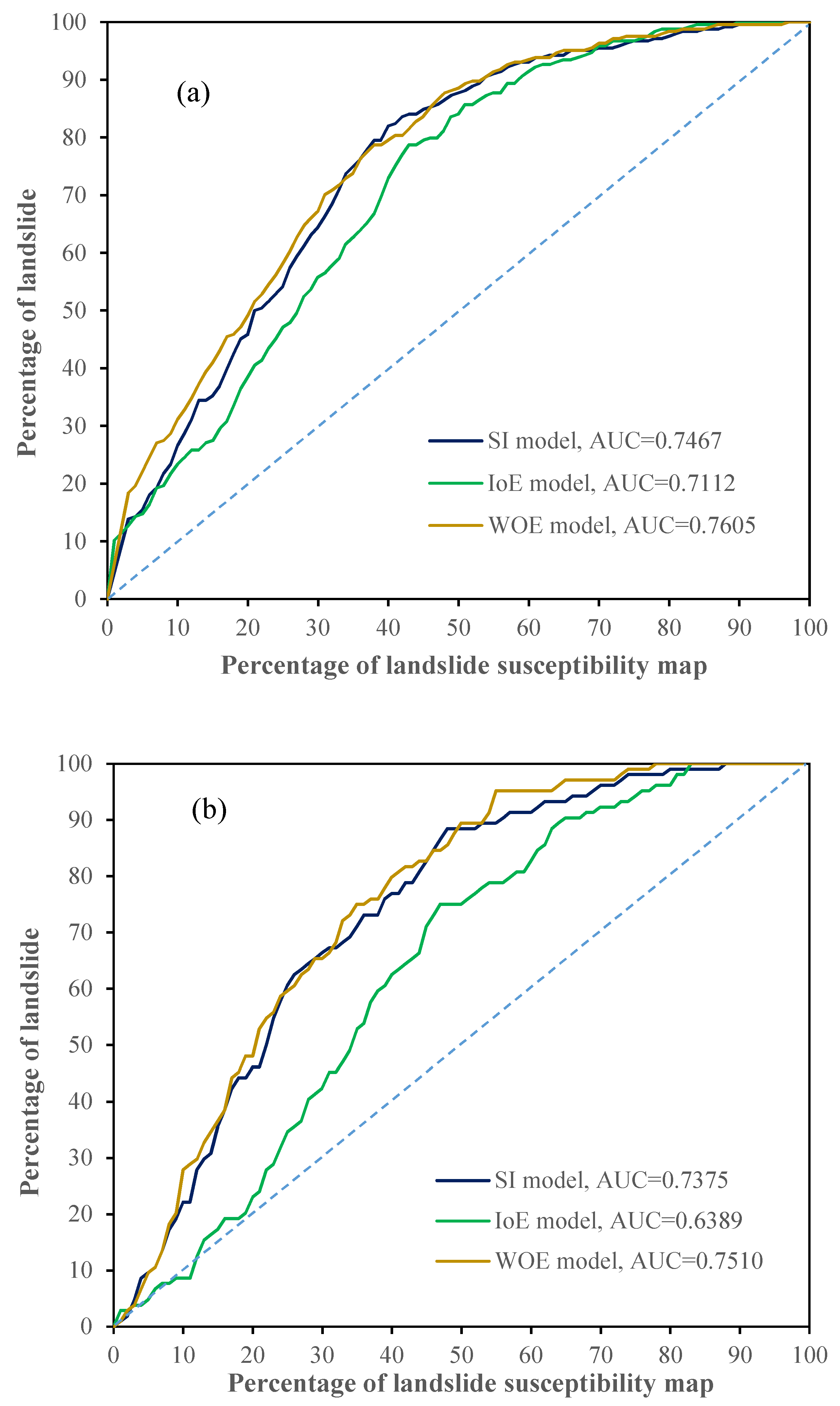
5.5. Validation and Comparison of the Models
6. Conclusions
Author Contributions
Funding
Conflicts of Interest
References
- Ambrosi, C.; Strozzi, T.; Scapozza, C.; Wegmüller, U. Landslide hazard assessment in the Himalayas (Nepal and Bhutan) based on Earth-Observation data. Eng. Geol. 2018, 237, 217–228. [Google Scholar] [CrossRef]
- Palmisano, F.; Vitone, C.; Cotecchia, F. Methodology for landslide damage assessment. Procedia Eng. 2016, 161, 511–515. [Google Scholar] [CrossRef]
- Zhou, C.; Yin, K.; Cao, Y.; Ahmed, B.; Li, Y.; Catani, F.; Pourghasemi, H.R. Landslide susceptibility modeling applying machine learning methods: A case study from Longju in the Three Gorges Reservoir area, China. Comput. Geosci. 2018, 112, 23–37. [Google Scholar] [CrossRef]
- Samodra, G.; Chen, G.; Sartohadi, J.; Kasama, K. Generating landslide inventory by participatory mapping: An example in Purwosari Area, Yogyakarta, Java. Geomorphology 2018, 306, 306–313. [Google Scholar] [CrossRef]
- Zhuang, J.; Peng, J.; Wang, G.; Javed, I.; Wang, Y.; Li, W. Distribution and characteristics of landslide in loess plateau: A case study in Shaanxi Province. Eng. Geol. 2018, 236, 89–96. [Google Scholar] [CrossRef]
- Chen, W.; Peng, J.; Hong, H.; Shahabi, H.; Pradhan, B.; Liu, J.; Zhu, A.-X.; Pei, X.; Duan, Z. Landslide susceptibility modelling using GIS-based machine learning techniques for Chongren county, Jiangxi Province, China. Sci. Total Environ. 2018, 626, 1121–1135. [Google Scholar] [CrossRef] [PubMed]
- Ciampalini, A.; Raspini, F.; Lagomarsino, D.; Catani, F.; Casagli, N. Landslide susceptibility map refinement using PSInSAR data. Remote Sens. Environ. 2016, 184, 302–315. [Google Scholar] [CrossRef] [Green Version]
- Huang, F.; Yin, K.; Huang, J.; Gui, L.; Wang, P. Landslide susceptibility mapping based on self-organizing-map network and extreme learning machine. Eng. Geol. 2017, 223, 11–22. [Google Scholar] [CrossRef]
- Lin, G.F.; Chang, M.J.; Huang, Y.C.; Ho, J.Y. Assessment of susceptibility to rainfall-induced landslides using improved self-organizing linear output map, support vector machine, and logistic regression. Eng. Geol. 2017, 224, 62–74. [Google Scholar] [CrossRef]
- Zêzere, J.L.; Pereira, S.; Melo, R.; Oliveira, S.C.; Garcia, R.A. Mapping landslide susceptibility using data-driven methods. Sci. Total Environ. 2017, 589, 250–267. [Google Scholar] [CrossRef] [PubMed]
- Goetz, J.N.; Brenning, A.; Petschko, H.; Leopold, P. Evaluating machine learning and statistical prediction techniques for landslide susceptibility modeling. Comput. Geosci. 2015, 81, 1–11. [Google Scholar] [CrossRef]
- Chen, W.; Pourghasemi, H.R.; Naghibi, S.A. Prioritization of landslide conditioning factors and its spatial modeling in Shangnan County, China using GIS-based data mining algorithms. Bull. Eng. Geol. Environ. 2018, 77, 611–629. [Google Scholar] [CrossRef]
- Mandal, S.; Mandal, K. Bivariate statistical index for landslide susceptibility mapping in the Rorachu river basin of eastern Sikkim Himalaya, India. Spat. Inf. Res. 2018, 26, 59–75. [Google Scholar] [CrossRef]
- Regmi, A.D.; Yoshida, K.; Pourghasemi, H.R.; DhitaL, M.R.; Pradhan, B. Landslide susceptibility mapping along Bhalubang–Shiwapur area of mid-Western Nepal using frequency ratio and conditional probability models. J. Mt. Sci. 2014, 11, 1266–1285. [Google Scholar] [CrossRef]
- Nicu, I.C. Application of analytic hierarchy process, frequency ratio, and statistical index to landslide susceptibility: An approach to endangered cultural heritage. Environ. Earth Sci. 2018, 77, 79. [Google Scholar] [CrossRef]
- Aditian, A.; Kubota, T.; Shinohara, Y. Comparison of GIS-based landslide susceptibility models using frequency ratio, logistic regression, and artificial neural network in a tertiary region of Ambon, Indonesia. Geomorphology 2018, 318, 101–111. [Google Scholar] [CrossRef]
- Althuwaynee, O.F.; Pradhan, B.; Park, H.-J.; Lee, J.H. A novel ensemble bivariate statistical evidential belief function with knowledge-based analytical hierarchy process and multivariate statistical logistic regression for landslide susceptibility mapping. Catena 2014, 114, 21–36. [Google Scholar] [CrossRef]
- Hong, H.; Kornejady, A.; Soltani, A.; Termeh, S.V.R.; Liu, J.; Zhu, A.X.; Hesar, A.Y.; Ahmad, B.B.; Wang, Y.C. Landslide susceptibility assessment in the Anfu County, China: comparing different statistical and probabilistic models considering the new topo-hydrological factor (HAND). Earth Sci. Inf. 2018, 1–18. [Google Scholar] [CrossRef]
- Chen, W.; Shahabi, H.; Shirzadi, A.; Li, T.; Guo, C.; Hong, H.; Li, W.; Pan, D.; Hui, J.; Ma, M.; et al. A novel ensemble approach of bivariate statistical based logistic model tree classifier for landslide susceptibility assessment. Geocarto Int. 2018, 1–32. [Google Scholar] [CrossRef]
- Razavizadeh, S.; Solaimani, K.; Massironi, M.; Kavian, A. Mapping landslide susceptibility with frequency ratio, statistical index, and weights of evidence models: A case study in Northern Iran. Environ. Earth Sci. 2017, 76, 499. [Google Scholar] [CrossRef]
- Ding, Q.; Chen, W.; Hong, H. Application of frequency ratio, weights of evidence and evidential belief function models in landslide susceptibility mapping. Geocarto Int. 2017, 32, 619–639. [Google Scholar] [CrossRef]
- Wang, L.-J.; Guo, M.; Sawada, K.; Lin, J.; Zhang, J. A comparative study of landslide susceptibility maps using logistic regression, frequency ratio, decision tree, weights of evidence and artificial neural network. Geosci. J. 2016, 20, 117–136. [Google Scholar] [CrossRef]
- Tahmassebipoor, N.; Rahmati, O.; Noormohamadi, F.; Lee, S. Spatial analysis of groundwater potential using weights-of-evidence and evidential belief function models and remote sensing. Arab. J. Geosci. 2016, 9, 1–18. [Google Scholar] [CrossRef]
- Bui, T.D.; Shahabi, H.; Shirzadi, A.; Chapi, K.; Alizadeh, M.; Chen, W.; Mohammadi, A.; Ahmad, B.; Panahi, M.; Hong, H.; et al. Landslide detection and susceptibility mapping by AIRSAR data using support vector machine and index of entropy models in Cameron Highlands, Malaysia. Remote Sens. 2018, 10, 1527. [Google Scholar]
- Chen, W.; Pourghasemi, H.R.; Naghibi, S.A. A comparative study of landslide susceptibility maps produced using support vector machine with different kernel functions and entropy data mining models in China. Bull. Eng. Geol. Environ. 2018, 77, 647–664. [Google Scholar] [CrossRef]
- Tsangaratos, P.; Ilia, I.; Hong, H.; Chen, W.; Xu, C. Applying information theory and GIS-based quantitative methods to produce landslide susceptibility maps in Nancheng County, China. Landslides 2017, 14, 1091–1111. [Google Scholar] [CrossRef]
- Youssef, A.M.; Al-Kathery, M.; Pradhan, B. Landslide susceptibility mapping at Al-Hasher area, Jizan (Saudi Arabia) using GIS-based frequency ratio and index of entropy models. Geosci. J. 2015, 19, 113–134. [Google Scholar] [CrossRef]
- Devkota, K.C.; Regmi, A.D.; Pourghasemi, H.R.; Yoshida, K.; Pradhan, B.; Ryu, I.C.; Dhital, M.R.; Althuwaynee, O.F. Landslide susceptibility mapping using certainty factor, index of entropy and logistic regression models in GIS and their comparison at Mugling–Narayanghat road section in Nepal Himalaya. Nat. Hazards 2013, 65, 135–165. [Google Scholar] [CrossRef] [Green Version]
- Trigila, A.; Iadanza, C.; Esposito, C.; Scarascia-Mugnozza, G. Comparison of logistic regression and random forests techniques for shallow landslide susceptibility assessment in Giampilieri (Ne Sicily, Italy). Geomorphology 2015, 249, 119–136. [Google Scholar] [CrossRef]
- Tsangaratos, P.; Ilia, I. Comparison of a logistic regression and naïve bayes classifier in landslide susceptibility assessments: The influence of models complexity and training dataset size. Catena 2016, 145, 164–179. [Google Scholar] [CrossRef]
- Chen, W.; Yan, X.; Zhao, Z.; Hong, H.; Bui, D.T.; Pradhan, B. Spatial prediction of landslide susceptibility using data mining-based kernel logistic regression, naive Bayes and RBFNetwork models for the Long County area (China). Bull. Eng. Geol. Environ. 2018, 1–20. [Google Scholar] [CrossRef]
- Pham, B.T.; Bui, T.D.; Pourghasemi, H.R.; Indra, P.; Dholakia, M. Landslide susceptibility assesssment in the Uttarakhand area (India) using GIS: A comparison study of prediction capability of naïve Bayes, multilayer perceptron neural networks, and functional trees methods. Theor. Appl. Climatol. 2017, 128, 255–273. [Google Scholar] [CrossRef]
- Chen, W.; Zhang, S.; Li, R.; Shahabi, H. Performance evaluation of the GIS-based data mining techniques of best-first decision tree, random forest, and naïve Bayes tree for landslide susceptibility modeling. Sci. Total Environ. 2018, 644, 1006–1018. [Google Scholar] [CrossRef]
- Chen, W.; Xie, X.; Peng, J.; Wang, J.; Duan, Z.; Hong, H. GIS-based landslide susceptibility modelling: A comparative assessment of kernel logistic regression, naïve-Bayes tree, and alternating decision tree models. Geomat. Nat. Hazards Risk 2017, 8, 950–973. [Google Scholar] [CrossRef]
- Pham, B.T.; Bui, T.D.; Prakash, I.; Dholakia, M.B. Evaluation of predictive ability of support vector machines and naive Bayes trees methods for spatial prediction of landslides in Uttarakhand state (India) using GIS. J. Geomat. 2016, 10, 71–79. [Google Scholar]
- Polykretis, C.; Chalkias, C. Comparison and evaluation of landslide susceptibility maps obtained from weight of evidence, logistic regression, and artificial neural network models. Nat. Hazards 2018, 36, 1–26. [Google Scholar] [CrossRef]
- Zhu, A.X.; Miao, Y.; Wang, R.; Zhu, T.; Deng, Y.; Liu, J.; Yang, L.; Qin, C.Z.; Hong, H. A comparative study of an expert knowledge-based model and two data-driven models for landslide susceptibility mapping. Catena 2018, 166, 317–327. [Google Scholar] [CrossRef]
- Bui, T.D.; Tuan, T.A.; Klempe, H.; Pradhan, B.; Revhaug, I. Spatial prediction models for shallow landslide hazards: A comparative assessment of the efficacy of support vector machines, artificial neural networks, kernel logistic regression, and logistic model tree. Landslides 2016, 13, 361–378. [Google Scholar]
- Hong, H.; Pradhan, B.; Xu, C.; Bui, T.D. Spatial prediction of landslide hazard at the Yihuang area (China) using two-class kernel logistic regression, alternating decision tree and support vector machines. Catena 2015, 133, 266–281. [Google Scholar] [CrossRef]
- Yao, X.; Tham, L.G.; Dai, F.C. Landslide susceptibility mapping based on support vector machine: A case study on natural slopes of Hong Kong, China. Geomorphology 2008, 101, 572–582. [Google Scholar] [CrossRef]
- Huang, Y.; Zhao, L. Review on landslide susceptibility mapping using support vector machines. Catena 2018, 165, 520–529. [Google Scholar] [CrossRef]
- Zhang, K.; Wu, X.; Niu, R.; Yang, K.; Zhao, L. The assessment of landslide susceptibility mapping using random forest and decision tree methods in the Three Gorges Reservoir area, China. Environ. Earth Sci. 2017, 76, 405. [Google Scholar] [CrossRef]
- Catani, F.; Lagomarsino, D.; Segoni, S.; Tofani, V. Landslide susceptibility estimation by random forests technique: Sensitivity and scaling issues. Nat. Hazards Earth Syst. Sci. 2013, 13, 2815–2831. [Google Scholar] [CrossRef]
- Pourghasemi, H.R.; Rossi, M. Landslide susceptibility modeling in a landslide prone area in Mazandarn Province, north of Iran: A comparison between GLM, GAM, MARS, and M-AHP methods. Theor. Appl. Climatol. 2017, 130, 609–633. [Google Scholar] [CrossRef]
- Conoscenti, C.; Ciaccio, M.; Caraballo-Arias, N.A.; Gómez-Gutiérrez, Á.; Rotigliano, E.; Agnesi, V. Assessment of susceptibility to earth-flow landslide using logistic regression and multivariate adaptive regression splines: A case of the Belice River basin (western Sicily, Italy). Geomorphology 2015, 242, 49–64. [Google Scholar] [CrossRef]
- Chen, W.; Panahi, M.; Pourghasemi, H.R. Performance evaluation of GIS-based new ensemble data mining techniques of adaptive neuro-fuzzy inference system (ANFIS) with genetic algorithm (GA), differential evolution (DE), and particle swarm optimization (PSO) for landslide spatial modelling. Catena 2017, 157, 310–324. [Google Scholar] [CrossRef]
- Pham, B.T.; Bui, T.D.; Prakash, I. Landslide susceptibility assessment using bagging ensemble based alternating decision trees, logistic regression and j48 decision trees methods: A comparative study. Geotech. Geol. Eng. 2017, 35, 2597–2611. [Google Scholar] [CrossRef]
- Hong, H.; Liu, J.; Bui, D.T.; Pradhan, B.; Acharya, T.D.; Pham, B.T.; Zhu, A.X.; Chen, W.; Ahmad, B.B. Landslide susceptibility mapping using j48 decision tree with adaboost, bagging and rotation forest ensembles in the Guangchang area (China). Catena 2018, 163, 399–413. [Google Scholar] [CrossRef]
- Bui, T.D.; Ho, T.-C.; Pradhan, B.; Pham, B.-T.; Nhu, V.-H.; Revhaug, I. GIS-based modeling of rainfall-induced landslides using data mining-based functional trees classifier with adaboost, bagging, and multiboost ensemble frameworks. Environ. Earth Sci. 2016, 75, 1–22. [Google Scholar]
- Aghdam, N.I.; Varzandeh, M.H.M.; Pradhan, B. Landslide susceptibility mapping using an ensemble statistical index (Wi) and adaptive neuro-fuzzy inference system (ANFIS) model at Alborz Mountains (Iran). Environ. Earth Sci. 2016, 75, 1–20. [Google Scholar] [CrossRef]
- Chen, W.; Panahi, M.; Tsangaratos, P.; Shahabi, H.; Ilia, I.; Panahi, S.; Li, S.; Jaafari, A.; Ahmad, B.B. Applying population-based evolutionary algorithms and a neuro-fuzzy system for modeling landslide susceptibility. Catena 2019, 172, 212–231. [Google Scholar] [CrossRef]
- Kornejady, A.; Ownegh, M.; Bahremand, A. Landslide susceptibility assessment using maximum entropy model with two different data sampling methods. Catena 2017, 152, 144–162. [Google Scholar] [CrossRef]
- Reichenbach, P.; Rossi, M.; Malamud, B.D.; Mihir, M.; Guzzetti, F. A review of statistically-based landslide susceptibility models. Earth Sci. Rev. 2018, 180, 60–91. [Google Scholar] [CrossRef]
- Guzzetti, F.; Mondini, A.C.; Cardinali, M.; Fiorucci, F.; Santangelo, M.; Chang, K.-T. Landslide inventory maps: New tools for an old problem. Earth Sci. Rev. 2012, 112, 42–66. [Google Scholar] [CrossRef]
- Hungr, O.; Leroueil, S.; Picarelli, L. The varnes classification of landslide types, an update. Landslides 2014, 11, 167–194. [Google Scholar] [CrossRef]
- Hong, H.; Ilia, I.; Tsangaratos, P.; Chen, W.; Xu, C. A hybrid fuzzy weight of evidence method in landslide susceptibility analysis on the Wuyuan area, China. Geomorphology 2017, 290, 1–16. [Google Scholar] [CrossRef]
- Pham, B.T.; Pradhan, B.; Bui, T.D.; Prakash, I.; Dholakia, M.B. A comparative study of different machine learning methods for landslide susceptibility assessment: A case study of Uttarakhand area (India). Environ. Model. Softw. 2016, 84, 240–250. [Google Scholar] [CrossRef]
- Ramakrishnan, D.; Singh, T.N.; Verma, A.K.; Gulati, A.; Tiwari, K.C. Soft computing and GIS for landslide susceptibility assessment in Tawaghat area, Kumaon Himalaya, India. Nat. Hazards 2013, 65, 315–330. [Google Scholar] [CrossRef]
- Caiyan, W.; Jianping, Q.; Meng, W. Landslides and slope aspect in the Three Gorges Reservoir area based on GIS and information value model. Wuhan Univ. J. Nat. Sci. 2006, 11, 773–779. [Google Scholar] [CrossRef]
- Paranunzio, R.; Laio, F.; Nigrelli, G.; Chiarle, M. A method to reveal climatic variables triggering slope failures at high elevation. Nat. Hazards 2015, 76, 1039–1061. [Google Scholar] [CrossRef]
- Chen, W.; Shahabi, H.; Shirzadi, A.; Hong, H.Y.; Akgun, A.; Tian, Y.Y.; Liu, J.Z.; Zhu, A.X.; Li, S.J. Novel hybrid artificial intelligence approach of bivariate statistical-methods-based kernel logistic regression classifier for landslide susceptibility modeling. Bull. Eng. Geol. Environ. 2018, 1–23. [Google Scholar] [CrossRef]
- Pourghasemi, H.R.; Pradhan, B.; Gokceoglu, C. Application of fuzzy logic and analytical hierarchy process (AHP) to landslide susceptibility mapping at Haraz Watershed, Iran. Nat. Hazards 2012, 63, 965–996. [Google Scholar] [CrossRef]
- Meten, M.; Prakashbhandary, N.; Yatabe, R. Effect of landslide factor combinations on the prediction accuracy of landslide susceptibility maps in the Blue Nile Gorge of Central Ethiopia. Geoenviron. Disasters 2015, 2, 9. [Google Scholar] [CrossRef]
- Ohlmacher, G.C. Plan curvature and landslide probability in regions dominated by earth flows and earth slides. Eng. Geol. 2007, 91, 117–134. [Google Scholar] [CrossRef]
- Chen, C.-Y.; Chang, J.-M. Landslide dam formation susceptibility analysis based on geomorphic features. Landslides 2016, 13, 1019–1033. [Google Scholar] [CrossRef]
- Kumar, R.; Anbalagan, R. Landslide susceptibility mapping using analytical hierarchy process (AHP) in Tehri reservoir rim region, Uttarakhand. J. Geol. Soc. India 2016, 87, 271–286. [Google Scholar] [CrossRef]
- Khorsandi, A.; Ghoreishi, S.H. Studying the interaction between active faults and landslide phenomenon: Case study of landslide in Latian, northeast Tehran, Iran. Geotech. Geol. Eng. 2013, 31, 617–625. [Google Scholar] [CrossRef]
- Li, X.-G.; Wang, A.-M.; Wang, Z.-M. Stability analysis and monitoring study of Jijia river landslide based on WeBGIS. J. Coal Sci. Eng. China 2010, 16, 41–46. [Google Scholar] [CrossRef]
- Ayalew, L.; Yamagishi, H. The application of GIS-based logistic regression for landslide susceptibility mapping in the Kakuda-Yahiko Mountains, Central Japan. Geomorphology 2005, 65, 15–31. [Google Scholar] [CrossRef]
- Gheshlaghi, H.A.; Feizizadeh, B. An integrated approach of analytical network process and fuzzy based spatial decision making systems applied to landslide risk mapping. J. Afr. Earth Sci. 2017, 133, 15–24. [Google Scholar] [CrossRef]
- Chen, W.; Xie, X.; Wang, J.; Pradhan, B.; Hong, H.; Bui, T.D.; Duan, Z.; Ma, J. A comparative study of logistic model tree, random forest, and classification and regression tree models for spatial prediction of landslide susceptibility. Catena 2017, 151, 147–160. [Google Scholar] [CrossRef]
- Dai, F.C.; Lee, C.F.; Li, J.; Xu, Z.W. Assessment of landslide susceptibility on the natural terrain of Lantau Island, Hong Kong. Environ. Geol. 2001, 40, 381–391. [Google Scholar]
- Koukis, G.; Pyrgiotis, L.; Kouki, A. Landslide phenomena in greece: Types of movement related to the lithology and structure of the geological formations. In Engineering Geology for Society and Territory: Landslide Processes; Lollino, G., Giordan, D., Crosta, G.B., Corominas, J., Azzam, R., Wasowski, J., Sciarra, N., Eds.; Springer International Publishing: Cham, Switzerland, 2015; Volume 2, pp. 1023–1027. [Google Scholar]
- Westen, C.J.V.; Rengers, N.; Terlien, M.T.J.; Soeters, R. Prediction of the occurrence of slope instability phenomenal through GIS-based hazard zonation. Geol. Rundsch. 1997, 86, 404–414. [Google Scholar] [CrossRef]
- Kayastha, P.; Dhital, M.R.; Smedt, F.D. Evaluation and comparison of GIS based landslide susceptibility mapping procedures in Kulekhani Watershed, Nepal. J. Geol. Soc. India 2013, 81, 219–231. [Google Scholar] [CrossRef]
- Regmi, A.D.; Devkota, K.C.; Yoshida, K.; Pradhan, B.; Pourghasemi, H.R.; Kumamoto, T.; Akgun, A. Application of frequency ratio, statistical index, and weights-of-evidence models and their comparison in landslide susceptibility mapping in Central Nepal Himalaya. Arab. J. Geosci. 2014, 7, 725–742. [Google Scholar] [CrossRef]
- Shi, Y.; Jin, F. Landslide stability analysis based on generalized information entropy. In Proceedings of the 2009 International Conference on Environmental Science and Information Application Technology, Wuhan, China, 4–5 July 2009; Volume 3, pp. 83–85. [Google Scholar]
- Bonham-Carter, G.E.; Cox, S. Geographic Information Systems for Geoscientists: Modelling with GIS; Elsevier: Amsterdam, The Netherlands, 2010; pp. 1–2. [Google Scholar]
- Chen, W.; Li, H.; Hou, E.; Wang, S.; Wang, G.; Panahi, M.; Li, T.; Peng, T.; Guo, C.; Niu, C.; et al. GIS-based groundwater potential analysis using novel ensemble weights-of-evidence with logistic regression and functional tree models. Sci. Total Environ. 2018, 634, 853–867. [Google Scholar] [CrossRef] [PubMed]
- Pham, B.T.; Prakash, I.; Bui, D.T. Spatial prediction of landslides using a hybrid machine learning approach based on random subspace and classification and regression trees. Geomorphology 2018, 303, 256–270. [Google Scholar] [CrossRef]
- Chen, W.; Xie, X.; Peng, J.; Shahabi, H.; Hong, H.; Bui, T.D.; Duan, Z.; Li, S.; Zhu, A.-X. GIS-based landslide susceptibility evaluation using a novel hybrid integration approach of bivariate statistical based random forest method. Catena 2018, 164, 135–149. [Google Scholar] [CrossRef]
- Witten, I.H.; Frank, E.; Mark, A.H. Data Mining: Practical Machine Learning Tools and Techniques, 3rd ed.; Morgan Kaufmann: Burlington, NJ, USA, 2011. [Google Scholar]
- Song, Y.; Gong, J.; Gao, S.; Wang, D.; Cui, T.; Li, Y.; Wei, B. Susceptibility assessment of earthquake-induced landslides using Bayesian network: A case study in Beichuan, China. Comput. Geosci. 2012, 42, 189–199. [Google Scholar] [CrossRef]
- Kohavi, R. A study of cross-validation and bootstrap for accuracy estimation and model selection. In Proceedings of the 14th International Joint Conference on Artificial Intelligence, Montreal, QC, Canada, 20–25 August 1995; pp. 1137–1143. [Google Scholar]
- Demir, G. Landslide susceptibility mapping by using statistical analysis in the North Anatolian Fault Zone (NAFZ) on the northern part of Suşehri Town, Turkey. Nat. Hazards 2018, 92, 133–154. [Google Scholar] [CrossRef]
- Lee, S.; Talib, J.A. Probabilistic landslide susceptibility and factor effect analysis. Environ. Geol. 2005, 47, 982–990. [Google Scholar] [CrossRef]
- Xie, Z.; Chen, G.; Meng, X.; Zhang, Y.; Qiao, L.; Tan, L. A comparative study of landslide susceptibility mapping using weight of evidence, logistic regression and support vector machine and evaluated by SBAS-InSAR monitoring: Zhouqu to Wudu segment in Bailong River Basin, China. Environ. Earth Sci. 2017, 76, 313. [Google Scholar] [CrossRef]
- Chen, W.; Pourghasemi, H.R.; Panahi, M.; Kornejady, A.; Wang, J.; Xie, X.; Cao, S. Spatial prediction of landslide susceptibility using an adaptive neuro-fuzzy inference system combined with frequency ratio, generalized additive model, and support vector machine techniques. Geomorphology 2017, 297, 69–85. [Google Scholar] [CrossRef]
- Pourghasemi, H.R.; Moradi, H.R.; Aghda, S.M.F. Landslide susceptibility mapping by binary logistic regression, analytical hierarchy process, and statistical index models and assessment of their performances. Nat. Hazards 2013, 69, 749–779. [Google Scholar] [CrossRef]
- Jenks, G.F. The data model concept in statistical mapping. Int. Yearb. Cartogr. 1967, 7, 186–190. [Google Scholar]
- Bijukchhen, S.M.; Kayastha, P.; Dhital, M.R. A comparative evaluation of heuristic and bivariate statistical modelling for landslide susceptibility mappings in Ghurmi–Dhad Khola, East Nepal. Arab. J. Geosci. 2013, 6, 2727–2743. [Google Scholar] [CrossRef]
- Chung, C.; Fabbri, A. Three Bayesian prediction models for landslide hazard. In Proceedings of the International Association for Mathematical Geology 1998 Annual Meeting (IAMG’98), Ischia, Italy, 4–9 October 1998; pp. 204–211. [Google Scholar]
- Chen, W.; Shirzadi, A.; Shahabi, H.; Ahmad, B.B.; Zhang, S.; Hong, H.; Zhang, N. A novel hybrid artificial intelligence approach based on the rotation forest ensemble and naïve Bayes tree classifiers for a landslide susceptibility assessment in Langao County, China. Geomat. Nat. Hazards Risk 2017, 8, 1955–1977. [Google Scholar] [CrossRef] [Green Version]
- Solaimani, K.; Mousavi, S.Z.; Kavian, A. Landslide susceptibility mapping based on frequency ratio and logistic regression models. Arab. J. Geosci. 2013, 6, 2557–2569. [Google Scholar] [CrossRef]


| Landslide Conditioning Factors | Average Merit (AM) | Standard Deviation (SD) |
|---|---|---|
| Distance to roads | 0.304 | ±0.021 |
| Elevation | 0.296 | ±0.027 |
| Distance to rivers | 0.260 | ±0.016 |
| Lithology | 0.156 | ±0.021 |
| Distance to faults | 0.155 | ±0.021 |
| TWI 1 | 0.083 | ±0.029 |
| Slope angle | 0.069 | ±0.027 |
| NDVI 2 | 0.060 | ±0.026 |
| Plan curvature | 0.056 | ±0.026 |
| SPI 3 | 0.035 | ±0.015 |
| Slope aspect | 0.032 | ±0.009 |
| STI 4 | 0.032 | ±0.022 |
| Profile curvature | 0.025 | ±0.027 |
| Conditioning Factors | Classes | No. of Pixels | No. of Landslide | SI | Wj | C |
|---|---|---|---|---|---|---|
| Slope angle (°) | 0–10 | 347,597 | 40 | 0.2023 | 0.0202 | 0.273 |
| 10–20 | 778,722 | 87 | 0.1728 | - | –0.001 | |
| 20–30 | 833,307 | 67 | –0.1562 | - | 0.029 | |
| 30–40 | 489,019 | 43 | –0.0667 | - | –0.234 | |
| 40–50 | 135,021 | 6 | –0.7492 | - | –0.155 | |
| 50–65 | 12,201 | 1 | –0.1370 | - | –0.143 | |
| Slope aspect | Flat | 167 | 0 | 0.000 | 0.0560 | 0.000 |
| North | 300,994 | 27 | –0.0467 | - | 0.028 | |
| Northeast | 318,751 | 32 | 0.0658 | - | 0.213 | |
| East | 345,947 | 44 | 0.3024 | - | 0.244 | |
| Southeast | 349,816 | 22 | –0.4019 | - | –0.309 | |
| South | 312,150 | 34 | 0.1474 | - | 0.170 | |
| Southwest | 333,799 | 24 | –0.2680 | - | –0.503 | |
| West | 320,387 | 31 | 0.0290 | - | 0.104 | |
| Northwest | 313,856 | 30 | 0.0168 | - | –0.101 | |
| Altitude (m) | <500 | 345,079 | 42 | 0.2584 | 0.1923 | 0.331 |
| 500–800 | 1,167,240 | 161 | 0.3835 | - | 0.842 | |
| 800–1100 | 688,633 | 32 | –0.7045 | - | –0.837 | |
| 1100–1400 | 350,308 | 9 | –1.2971 | - | –1.656 | |
| 1400–1700 | 38,955 | 0 | 0.000 | - | –1.287 | |
| >2050 | 5652 | 0 | 0.000 | - | 0.000 | |
| Plan curvature | –9.57 to –1.09 | 265,054 | 23 | –0.0799 | 0.0006 | –0.043 |
| –1.09 to –0.11 | 872,136 | 83 | 0.0124 | - | –0.036 | |
| –0.11 to 0.88 | 1,046,545 | 101 | 0.0264 | - | 0.130 | |
| 0.88–11.42 | 412,132 | 37 | -0.0459 | - | –0.155 | |
| Profile curvature | –11.93 to –1.30 | 285,207 | 21 | –0.2442 | 0.0053 | –0.216 |
| –1.30 to –0.02 | 950,381 | 88 | –0.0150 | - | –0.060 | |
| –0.02 to –1.26 | 1,047,612 | 103 | 0.0450 | - | 0.108 | |
| 1.26–11.43 | 312,667 | 32 | 0.0851 | - | 0.064 | |
| SPI | 0–30 | 1,256,999 | 128 | 0.0801 | 0.0022 | 0.264 |
| 30–60 | 499,682 | 44 | –0.0653 | - | –0.355 | |
| 60–90 | 243,080 | 23 | 0.0066 | - | 0.053 | |
| >90 | 596,106 | 49 | –0.1341 | - | –0.123 | |
| STI | 0–10 | 963,339 | 99 | 0.0892 | 0.0063 | –0.137 |
| 10–20 | 723,470 | 70 | 0.0289 | - | 0.177 | |
| 20–30 | 392,792 | 38 | 0.0288 | - | –0.059 | |
| >30 | 516,266 | 37 | –0.2712 | - | –0.149 | |
| TWI | <5 | 1,095,483 | 91 | –0.1236 | 0.0090 | 0.235 |
| 5–7 | 1,131,652 | 117 | 0.0952 | - | –0.171 | |
| 7–9 | 258,581 | 28 | 0.1415 | - | 0.031 | |
| >9 | 110,151 | 8 | –0.2579 | - | –0.180 | |
| Distance to faults (m) | 0–1000 | 1,353,065 | 170 | 0.2902 | 0.1068 | 0.739 |
| 1000–2000 | 596,473 | 55 | –0.0192 | - | –0.025 | |
| 2000–3000 | 219,389 | 13 | –0.4614 | - | –0.486 | |
| 3000–4000 | 99,497 | 2 | –1.5425 | - | –1.564 | |
| >4000 | 327,420 | 4 | –2.0405 | - | –2.151 | |
| Distance to rivers (m) | <200 | 1,099,425 | 139 | 0.2964 | 0.0511 | 0.530 |
| 200–400 | 770,613 | 72 | –0.0060 | - | 0.065 | |
| 400–600 | 405,048 | 19 | –0.6951 | - | –0.781 | |
| 600–800 | 163,814 | 6 | –0.9425 | - | –1.160 | |
| >800 | 156,944 | 8 | –0.6119 | -- | –0.606 | |
| Distance to roads (m) | <500 | 696,109 | 113 | 0.5464 | 0.0546 | 0.850 |
| 500–1000 | 547,849 | 42 | –0.2038 | - | –0.228 | |
| 1000–1500 | 439,072 | 39 | –0.0566 | - | –0.102 | |
| 1500–2000 | 334,495 | 17 | –0.6149 | - | –0.681 | |
| >2000 | 578,319 | 33 | –0.4991 | - | –0.590 | |
| NDVI | –0.23 to 0.17 | 64,496 | 8 | 0.2773 | 0.0145 | –0.439 |
| 0.17–0.33 | 232,432 | 17 | –0.2509 | - | 0.107 | |
| 0.33–0.42 | 713,855 | 66 | –0.0165 | - | –0.081 | |
| 0.42–0.51 | 965,450 | 78 | –0.1514 | - | –0.028 | |
| 0.51–0.71 | 619,630 | 75 | 0.2529 | - | 0.106 | |
| Lithology | Harder metamorphic rocks | 514,860 | 29 | –0.5121 | 0.0954 | –0.824 |
| Softer metamorphic rocks | 771,447 | 141 | 0.6650 | - | –0.606 | |
| Hard carbonate rocks | 734,975 | 43 | –0.4742 | - | 0.361 | |
| Hard intrusive rocks | 522,464 | 24 | –0.7160 | - | 1.159 | |
| Soft gravelly soils | 52,038 | 7 | 0.3584 | - | –0.607 |
© 2018 by the authors. Licensee MDPI, Basel, Switzerland. This article is an open access article distributed under the terms and conditions of the Creative Commons Attribution (CC BY) license (http://creativecommons.org/licenses/by/4.0/).
Share and Cite
Liu, J.; Duan, Z. Quantitative Assessment of Landslide Susceptibility Comparing Statistical Index, Index of Entropy, and Weights of Evidence in the Shangnan Area, China. Entropy 2018, 20, 868. https://0-doi-org.brum.beds.ac.uk/10.3390/e20110868
Liu J, Duan Z. Quantitative Assessment of Landslide Susceptibility Comparing Statistical Index, Index of Entropy, and Weights of Evidence in the Shangnan Area, China. Entropy. 2018; 20(11):868. https://0-doi-org.brum.beds.ac.uk/10.3390/e20110868
Chicago/Turabian StyleLiu, Jie, and Zhao Duan. 2018. "Quantitative Assessment of Landslide Susceptibility Comparing Statistical Index, Index of Entropy, and Weights of Evidence in the Shangnan Area, China" Entropy 20, no. 11: 868. https://0-doi-org.brum.beds.ac.uk/10.3390/e20110868