Hybrid Integration Approach of Entropy with Logistic Regression and Support Vector Machine for Landslide Susceptibility Modeling


Abstract
:1. Introduction
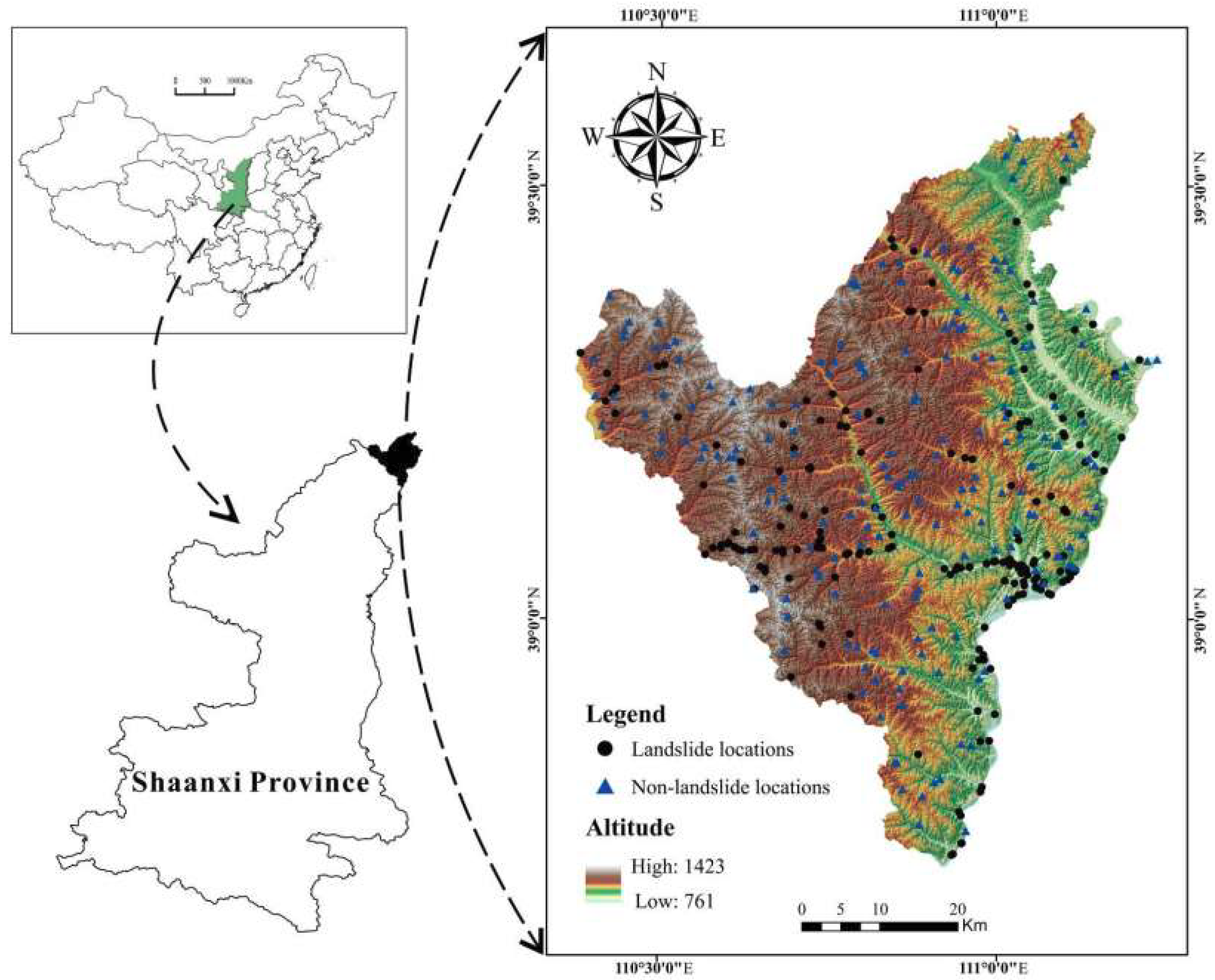
2. Study Area
3. Data Used
3.1. Landslide Inventory Map
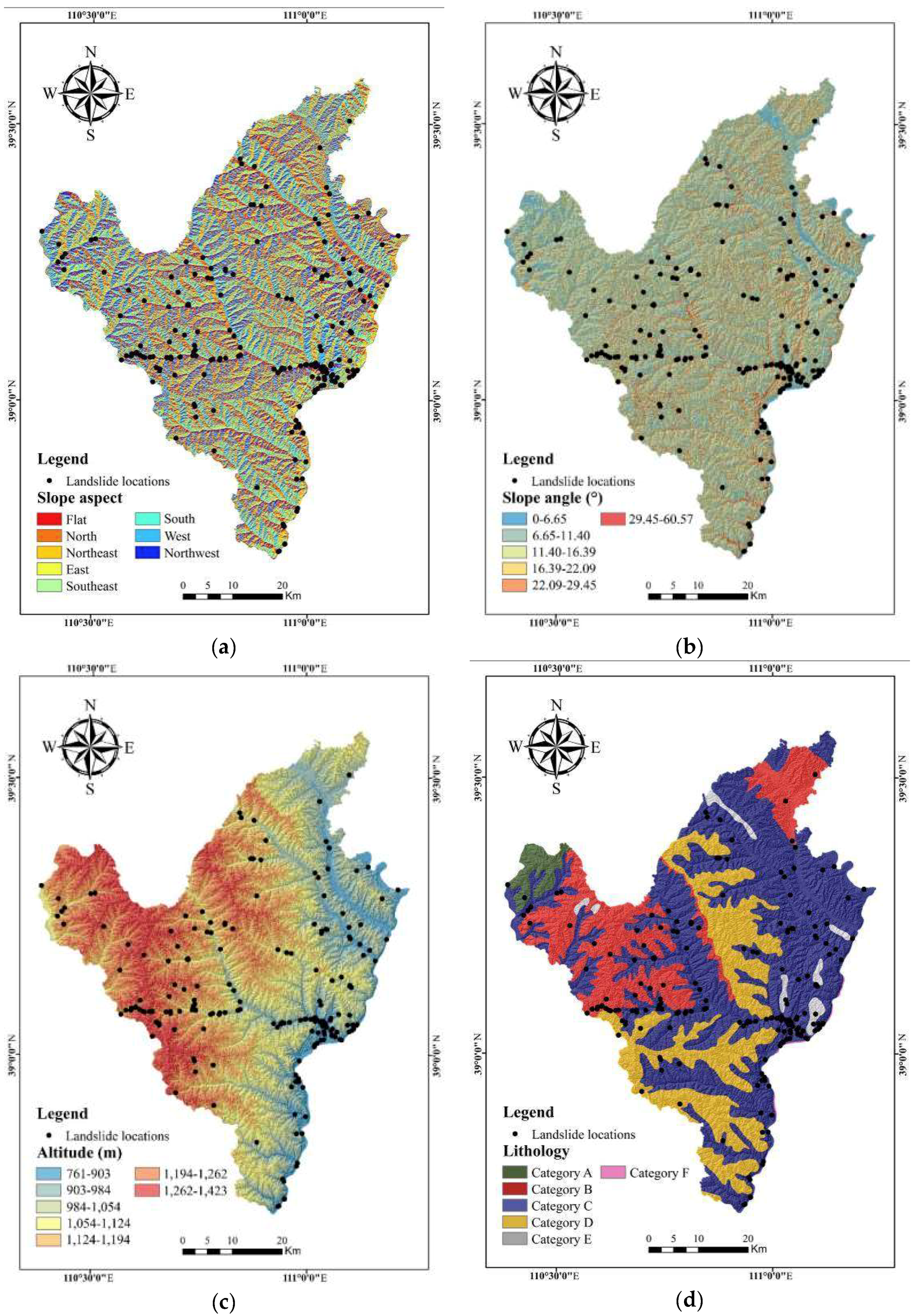
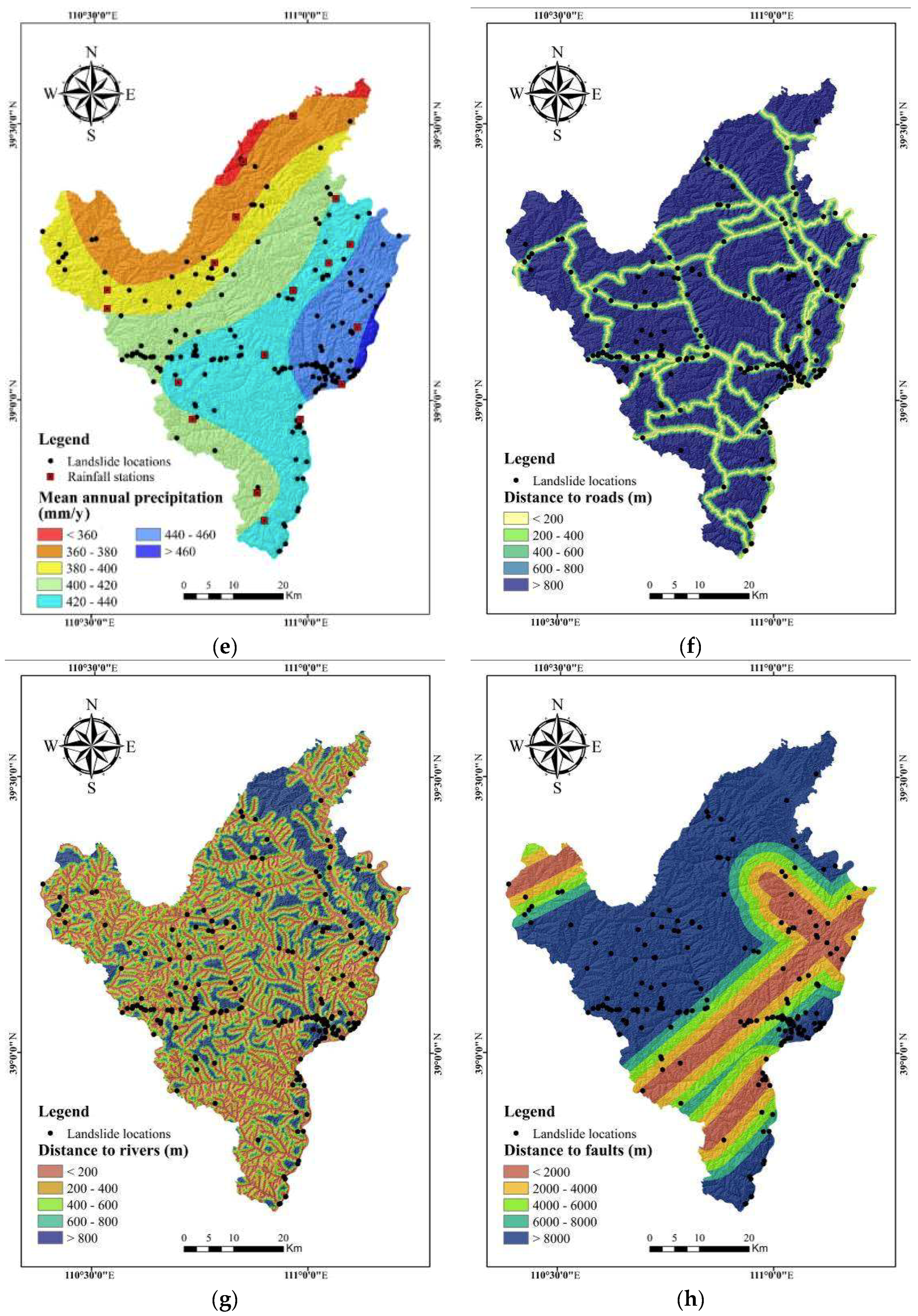
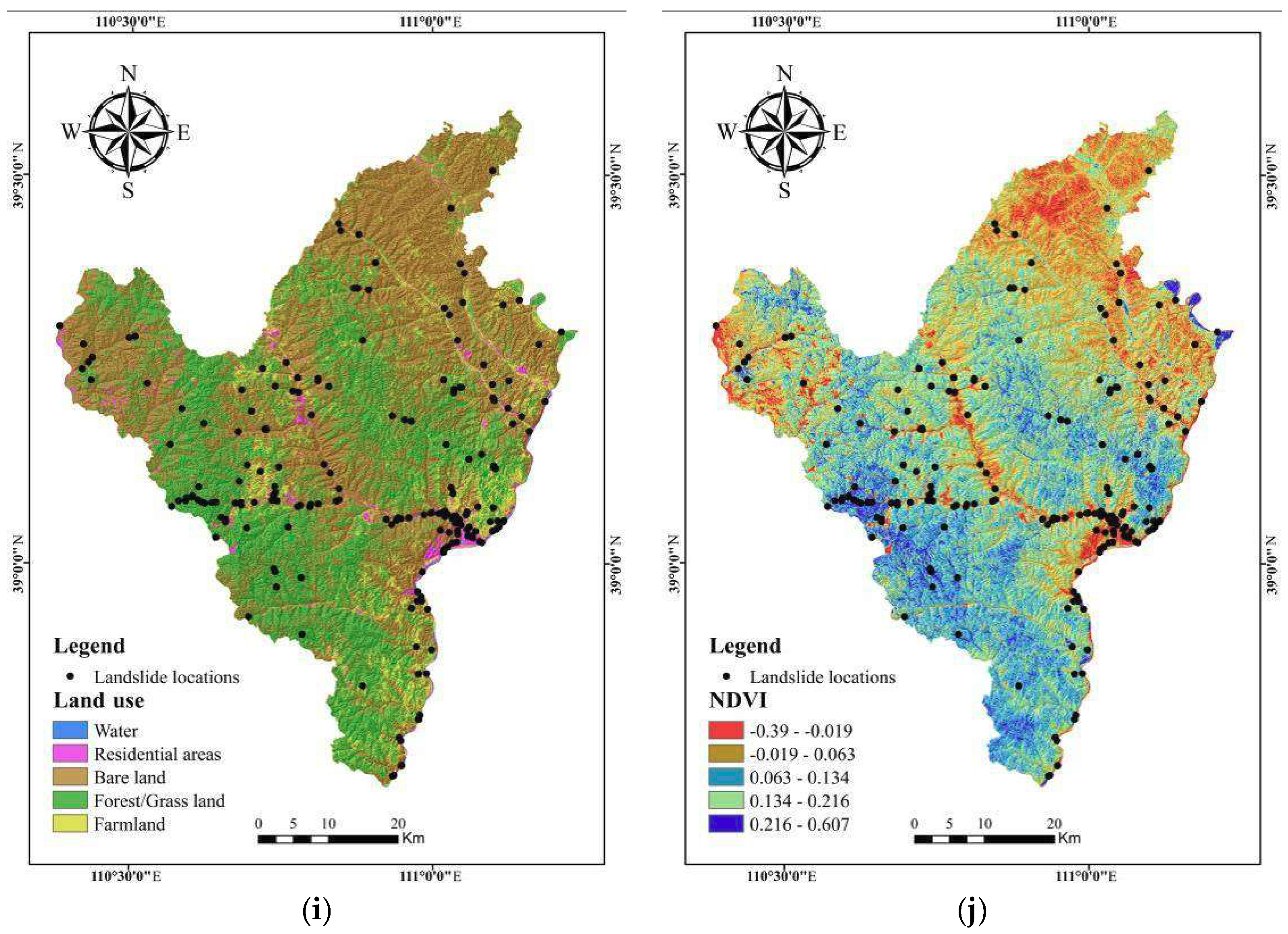
3.2. Landslide Explanatory Variables
4. Methodologies
4.1. Multicollinearity Diagnosis
4.2. Index of Entropy (IOE) Method
4.3. Integration of Logistic Regression and Index of Entropy Model
4.4. Integration of Support Vector Machine and Index of Entropy Model
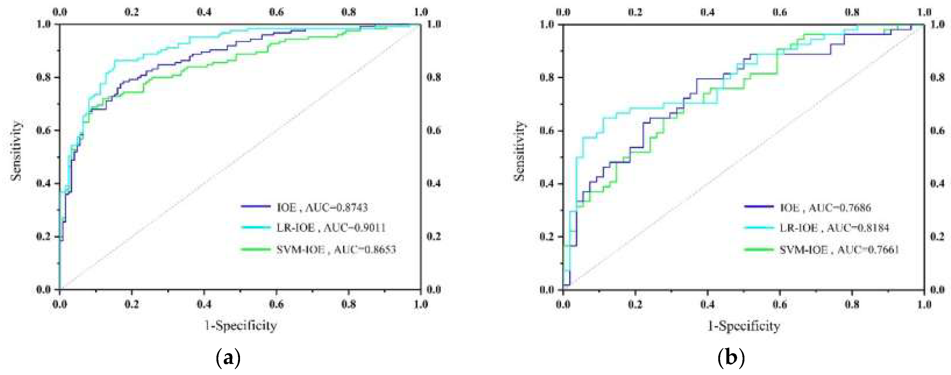
4.5. The ROC Curve
5. Results
5.1. Assessment of Explanatory Variables
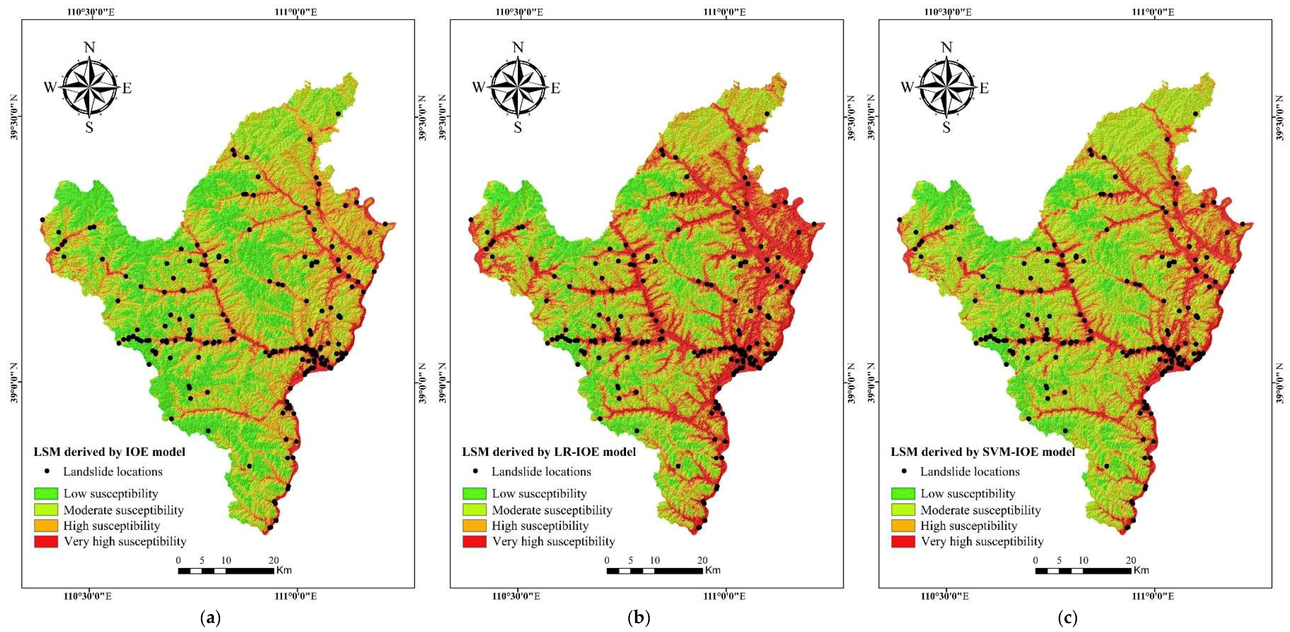
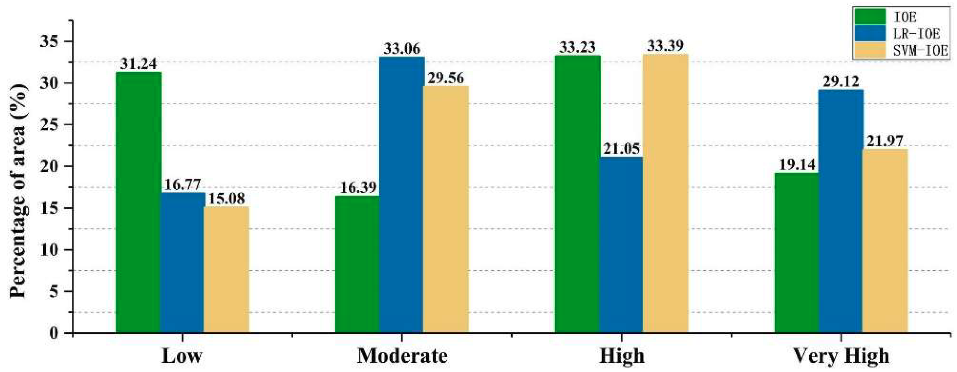
5.2. Result of IOE Model
5.3. Result of LR–IOE Model
5.4. Result of SVM–IOE Model
5.5. Validation of Landslide Susceptibility Maps
6. Discussion
7. Conclusions
Author Contributions
Funding
Acknowledgments
Conflicts of Interest
References
- Akgun, A.; Erkan, O. Landslide susceptibility mapping by geographical information system-based multivariate statistical and deterministic models: In an artificial reservoir area at northern Turkey. Arab. J. Geosci. 2016, 9, 1–15. [Google Scholar] [CrossRef]
- Petley, D. Global patterns of loss of life from landslides. Geology 2012, 40, 927–930. [Google Scholar] [CrossRef]
- National Statistics on Geological Disasters in 2017. Available online: www.jianzai.gov.cn (accessed on 25 October 2018).
- Brabb, E.E. Innovative approaches to landslide hazard mapping. In Proceedings of the IV International Symposium on Landslides, Toronto, Canada, 23–31 August 1985; Volume 1, pp. 307–324. [Google Scholar]
- Yin, K. The computer-assisted mapping of landslide hazard zonation. Hydrogeol. Eng. Geol 1993, 5, 21–23. [Google Scholar]
- Brabb, E.E. The San Mateo County California Gis Project for Predicting the Consequences of Hazardous Geologic Processes. In Geographical Information Systems in Assessing Natural Hazards; Springer: Dordrecht, The Netherlands, 1995. [Google Scholar]
- Pourghasemi, H.R.; Pradhan, B.; Gokceoglu, C. Application of fuzzy logic and analytical hierarchy process (AHP) to landslide susceptibility mapping at Haraz watershed, Iran. Nat. Hazards 2012, 63, 965–996. [Google Scholar] [CrossRef]
- Yilmaz, I. Landslide susceptibility mapping using frequency ratio, logistic regression, artificial neural networks and their comparison: A case study from Kat landslides (Tokat-Turkey). Comput. Geosci. 2009, 35, 1125–1138. [Google Scholar] [CrossRef]
- Pradhan, B. Landslide susceptibility mapping of a catchment area using frequency ratio, fuzzy logic and multivariate logistic regression approaches. J. Indian Soc. Remote Sens. 2010, 38, 301–320. [Google Scholar] [CrossRef]
- Akinci, H.; Doğan, S.; Kilicoğlu, C.; Temiz, M.S. Production of landslide susceptibility map of Samsun (Turkey) city center by using frequency ratio method. Int. J. Phys. Sci. 2011, 6, 1015–1025. [Google Scholar]
- Mondal, S.; Maiti, R. Integrating the analytical hierarchy process (AHP) and the frequency ratio (FR) model in landslide susceptibility mapping of Shiv-Khola watershed, Darjeeling Himalaya. Int. J. Disaster Risk Sci. 2013, 4, 200–212. [Google Scholar] [CrossRef]
- Vakhshoori, V.; Zare, M. Landslide susceptibility mapping by comparing weight of evidence, fuzzy logic, and frequency ratio methods. Geomatics 2016, 7, 1–21. [Google Scholar] [CrossRef] [Green Version]
- Dev, T.; Tae, I.; Ha, D. GIS-based landslide susceptibility mapping of Bhotang, Nepal using frequency ratio and statistical index methods. J. Korean Soc. Surv. Geod. Photogramm. Cartogr. 2017, 35, 357–364. [Google Scholar]
- Devkota, K.C.; Regmi, A.D.; Pourghasemi, H.R.; Yoshida, K.; Pradhan, B.; Ryu, I.C.; Dhital, M.R.; Althuwaynee, O.F. Landslide susceptibility mapping using certainty factor, index of entropy and logistic regression models in GIS and their comparison at Mugling-Narayanghat road section in Nepal Himalaya. Nat. Hazards 2013, 65, 135–165. [Google Scholar] [CrossRef] [Green Version]
- Pourghasemi, H.R.; Pradhan, B.; Gokceoglu, C.; Mohammadi, M.; Moradi, H.R. Application of weights-of-evidence and certainty factor models and their comparison in landslide susceptibility mapping at Haraz watershed, Iran. Arab. J. Geosci. 2013, 6, 2351–2365. [Google Scholar] [CrossRef] [Green Version]
- Wang, Q.; Li, W.; Chen, W.; Bai, H. GIS-based assessment of landslide susceptibility using certainty factor and index of entropy models for the Qianyang County of Baoji City, China. J. Earth Syst. Sci. 2015, 124, 1–17. [Google Scholar] [CrossRef]
- Hong, H.; Chen, W.; Xu, C.; Youssef, A.M.; Pradhan, B.; Bui, D.T. Rainfall-induced landslide susceptibility assessment at the Chongren area (China) using frequency ratio, certainty factor, and index of entropy. Geocarto Int. 2017, 32, 139–154. [Google Scholar] [CrossRef]
- Bui, D.T.; Lofman, O.; Revhaug, I.; Dick, O. Landslide susceptibility analysis in the Hoa Binh province of Vietnam using statistical index and logistic regression. Nat. Hazards 2011, 59, 1413–1444. [Google Scholar] [CrossRef]
- Pourghasemi, H.R.; Moradi, H.R.; Aghda, S.M.F. Landslide susceptibility mapping by binary logistic regression, analytical hierarchy process, and statistical index models and assessment of their performances. Nat. Hazards 2013, 69, 749–779. [Google Scholar] [CrossRef]
- Polykretis, C.; Chalkias, C. Comparison and evaluation of landslide susceptibility maps obtained from weight of evidence, logistic regression, and artificial neural network models. Nat. Hazards 2018, 93, 1–26. [Google Scholar] [CrossRef]
- Ilia, I.; Tsangaratos, P. Applying weight of evidence method and sensitivity analysis to produce a landslide susceptibility map. Landslides 2016, 13, 379–397. [Google Scholar] [CrossRef]
- Chen, W.; Li, H.; Hou, E.; Wang, S.; Wang, G.; Panahi, M.; Li, T.; Peng, T.; Guo, C.; Niu, C. GIS-based groundwater potential analysis using novel ensemble weights-of-evidence with logistic regression and functional tree models. Sci. Total Environ. 2018, 634, 853. [Google Scholar] [CrossRef] [PubMed]
- Pourghasemi, H.R.; Mohammady, M.; Pradhan, B. Landslide susceptibility mapping using index of entropy and conditional probability models in GIS: Safarood Basin, Iran. Catena 2012, 97, 71–84. [Google Scholar] [CrossRef]
- Razavizadeh, S.; Solaimani, K.; Massironi, M.; Kavian, A. Mapping landslide susceptibility with frequency ratio, statistical index, and weights of evidence models: A case study in northern Iran. Environ. Earth Sci. 2017, 76, 499. [Google Scholar] [CrossRef]
- Manzo, G.; Tofani, V.; Segoni, S.; Battistini, A.; Catani, F. GIS techniques for regional-scale landslide susceptibility assessment: The Sicily (Italy) case study. Int. J. Geogr. Inf. Sci. 2013, 27, 1433–1452. [Google Scholar] [CrossRef]
- Chen, W.; Shahabi, H.; Shirzadi, A.; Hong, H.Y.; Akgun, A.; Tian, Y.Y.; Liu, J.Z.; Zhu, A.X.; Li, S.J. Novel hybrid artificial intelligence approach of bivariate statistical-methods-based kernel logistic regression classifier for landslide susceptibility modeling. Bull. Eng. Geol. Environ. 2018, 1–23. [Google Scholar] [CrossRef]
- Trigila, A.; Iadanza, C.; Esposito, C.; Scarascia-Mugnozza, G. Comparison of logistic regression and random forests techniques for shallow landslide susceptibility assessment in Giampilieri (NE Sicily, Italy). Geomorphology 2015, 249, 119–136. [Google Scholar] [CrossRef]
- Saro, L.; Woo, J.S.; Kwanyoung, O.; Moungjin, L. The spatial prediction of landslide susceptibility applying artificial neural network and logistic regression models: A case study of Inje, Korea. Open Geosci. 2016, 8, 117–132. [Google Scholar] [CrossRef]
- Tsangaratos, P.; Ilia, I. Comparison of a logistic regression and naïve bayes classifier in landslide susceptibility assessments: The influence of models complexity and training dataset size. Catena 2016, 145, 164–179. [Google Scholar] [CrossRef]
- Mandal, S.; Mandal, K. Modeling and mapping landslide susceptibility zones using GIS based multivariate binary logistic regression (LR) model in the Rorachu river basin of eastern Sikkim Himalaya, India. Model. Earth Syst. Environ. 2018, 4, 69–88. [Google Scholar] [CrossRef]
- Lin, H.M.; Chang, S.K.; Wu, J.H.; Juang, C.H. Neural network-based model for assessing failure potential of highway slopes in the Alishan, Taiwan Area: Pre- and post-earthquake investigation. Eng. Geol. 2009, 104, 280–289. [Google Scholar] [CrossRef]
- Conforti, M.; Pascale, S.; Robustelli, G.; Sdao, F. Evaluation of prediction capability of the artificial neural networks for mapping landslide susceptibility in the Turbolo river catchment (northern Calabria, Italy). Catena 2014, 113, 236–250. [Google Scholar] [CrossRef]
- Aditian, A.; Kubota, T. Causative factors optimization using artificial neural network for GIS-based landslide susceptibility assessments in Ambon, Indonesia. Int. J. Eros. Control Eng. 2017, 10, 120–129. [Google Scholar] [CrossRef]
- Oh, H.J.; Pradhan, B. Application of a neuro-fuzzy model to landslide-susceptibility mapping for shallow landslides in a tropical hilly area. Comput. Geosci. 2011, 37, 1264–1276. [Google Scholar] [CrossRef]
- Lee, M.J.; Park, I.; Lee, S. Forecasting and validation of landslide susceptibility using an integration of frequency ratio and neuro-fuzzy models: A case study of Seorak mountain area in Korea. Environ. Earth Sci. 2015, 74, 413–429. [Google Scholar] [CrossRef]
- Chen, W.; Pourghasemi, H.R.; Panahi, M.; Kornejady, A.; Wang, J.; Xie, X. Spatial prediction of landslide susceptibility using an adaptive neuro-fuzzy inference system combined with frequency ratio, generalized additive model, and support vector machine techniques. Geomorphology 2017, 297, 69–85. [Google Scholar] [CrossRef]
- Chen, W.; Panahi, M.; Tsangaratos, P.; Shahabi, H.; Ilia, I.; Panahi, S.; Li, S.; Jaafari, A.; Ahmad, B.B. Applying population-based evolutionary algorithms and a neuro-fuzzy system for modeling landslide susceptibility. Catena 2019, 172, 212–231. [Google Scholar] [CrossRef]
- Anbalagan, R.; Kumar, R.; Lakshmanan, K.; Parida, S.; Neethu, S. Landslide hazard zonation mapping using frequency ratio and fuzzy logic approach, a case study of Lachung valley, Sikkim. Geoenviron. Disasters 2015, 2, 1–17. [Google Scholar] [CrossRef]
- Tsangaratos, P.; Loupasakis, C.; Nikolakopoulos, K.; Angelitsa, V.; Ilia, I. Developing a landslide susceptibility map based on remote sensing, fuzzy logic and expert knowledge of the island of Lefkada, Greece. Environ. Earth Sci. 2018, 77, 363. [Google Scholar] [CrossRef]
- Pradhan, B. A comparative study on the predictive ability of the decision tree, support vector machine and neuro-fuzzy models in landslide susceptibility mapping using GIS. Comput. Geosci. 2013, 51, 350–365. [Google Scholar] [CrossRef] [Green Version]
- Bui, D.T.; Pradhan, B.; Lofman, O.; Revhaug, I. Landslide susceptibility assessment in Vietnam using support vector machines, decision tree, and naı¨ve bayes models. Math. Probl. Eng. 2012, 2012. [Google Scholar]
- Lombardo, L.; Cama, M.; Conoscenti, C.; Märker, M.; Rotigliano, E. Binary logistic regression versus stochastic gradient boosted decision trees in assessing landslide susceptibility for multiple-occurring landslide events: Application to the 2009 storm event in Messina (Sicily, southern Italy). Nat. Hazards 2015, 79, 1621–1648. [Google Scholar] [CrossRef]
- Hong, H.; Pradhan, B.; Xu, C.; Bui, D.T. Spatial prediction of landslide hazard at the Yihuang area (China) using two-class kernel logistic regression, alternating decision tree and support vector machines. Catena 2015, 133, 266–281. [Google Scholar] [CrossRef]
- Chen, W.; Xie, X.; Peng, J.; Wang, J.; Duan, Z.; Hong, H. GIS-based landslide susceptibility modelling: A comparative assessment of kernel logistic regression, Naïve-Bayes tree, and alternating decision tree models. Geomat. Nat. Hazards Risk 2017, 8, 950–973. [Google Scholar] [CrossRef]
- Colkesen, I.; Sahin, E.K.; Kavzoglu, T. Susceptibility mapping of shallow landslides using kernel-based gaussian process, support vector machines and logistic regression. J. Afr. Earth Sci. 2016, 118, 53–64. [Google Scholar] [CrossRef]
- Lee, S.; Hong, S.M.; Jung, H.S. A support vector machine for landslide susceptibility mapping in Gangwon province, Korea. Sustainability 2017, 9, 48. [Google Scholar] [CrossRef]
- Huang, Y.; Zhao, L. Review on landslide susceptibility mapping using support vector machines. Catena 2018, 165, 520–529. [Google Scholar] [CrossRef]
- Chen, W.; Shahabi, H.; Shirzadi, A.; Li, T.; Guo, C.; Hong, H.; Li, W.; Pan, D.; Hui, J.; Ma, M. A Novel Ensemble Approach of Bivariate Statistical Based Logistic Model Tree Classifier for Landslide Susceptibility Assessment. Geocarto Int. 2018, 1–32. [Google Scholar] [CrossRef]
- Chen, W.; Xie, X.; Peng, J.; Himan, S.; Hong, H.; Bui, D.T. GIS-based landslide susceptibility evaluation using a novel hybrid integration approach of bivariate statistical based random forest method. Catena 2018, 164, 135–149. [Google Scholar] [CrossRef]
- Eeckhaut, M.V.D. Statistical modelling of Europe-wide landslide susceptibility using limited landslide inventory data. Landslides 2012, 9, 357–369. [Google Scholar] [CrossRef]
- Trigila, A.; Frattini, P.; Casagli, N.; Catani, F.; Crosta, G.; Esposito, C.; Iadanza, C.; Lagomarsino, D.; Mugnozza, G.S.; Segoni, S. Landslide Susceptibility Mapping at National Scale: The Italian Case Study. In Landslide Science and Practice; Springer: Berlin, Germany, 2015; pp. 287–295. [Google Scholar]
- Aghdam, I.N.; Pradhan, B.; Panahi, M. Landslide susceptibility assessment using a novel hybrid model of statistical bivariate methods (FR and WOE) and adaptive neuro-fuzzy inference system (ANFIS) at southern Zagros mountains in Iran. Environ. Earth Sci. 2017, 76, 237. [Google Scholar] [CrossRef]
- Moosavi, V.; Niazi, Y. Development of hybrid wavelet packet-statistical models (WP-SM) for landslide susceptibility mapping. Landslides 2016, 13, 1–18. [Google Scholar] [CrossRef]
- Pham, B.T.; Jaafari, A.; Prakash, I.; Bui, D.T. A novel hybrid intelligent model of support vector machines and the multiboost ensemble for landslide susceptibility modeling. Bull. Eng. Geol. Environ. 2018, 47, 1–22. [Google Scholar] [CrossRef]
- Guzzetti, F.; Mondini, A.C.; Cardinali, M.; Fiorucci, F.; Santangelo, M.; Chang, K.T. Landslide inventory maps: New tools for an old problem. Earth Sci. Rev. 2012, 112, 42–66. [Google Scholar] [CrossRef]
- Geospatial Data Cloud. Available online: https://http://www.gscloud.cn/ (accessed on 25 September 2018).
- Dou, J.; Yamagishi, H.; Pourghasemi, H.R.; Yunus, A.P.; Song, X.; Xu, Y. An integrated artificial neural network model for the landslide susceptibility assessment of Osado island, Japan. Nat. Hazards 2015, 78, 1749–1776. [Google Scholar] [CrossRef]
- Chen, W.; Peng, J.; Hong, H.; Shahabi, H.; Pradhan, B.; Liu, J. Landslide susceptibility modelling using GIS-based machine learning techniques for Chongren county, Jiangxi province, China. Sci. Total Environ. 2018, 626, 230. [Google Scholar] [CrossRef] [PubMed]
- Nakamura, H.; Kubota, T. Landslide susceptibility from the viewpoint of its slope angle and geology. J. Jpn. Landslide Soc. 2010, 23, 6–12_1. [Google Scholar] [CrossRef]
- Westen, C.J.V.; Rengers, N.; Soeters, R. Use of geomorphological information in indirect landslide susceptibility assessment. Nat. Hazards 2003, 30, 399–419. [Google Scholar] [CrossRef]
- Dahal, R.K.; Hasegawa, S.; Nonomura, A.; Yamanaka, M.; Masuda, T.; Nishino, K. GIS-based weights-of-evidence modelling of rainfall-induced landslides in small catchments for landslide susceptibility mapping. Environ. Geol. 2008, 54, 311–324. [Google Scholar] [CrossRef]
- Youssef, A.M. Landslide susceptibility delineation in the Ar-Rayth area, Jizan, kingdom of Saudi Arabia, using analytical hierarchy process, frequency ratio, and logistic regression models. Environ. Earth Sci. 2015, 73, 1–20. [Google Scholar] [CrossRef]
- Chang, S.K.; Lee, D.H.; Wu, J.H.; Juang, C.H. Rainfall-based criteria for assessing slump rate of mountainous highway slopes: A case study of slopes along Highway 18 in Alishan, Taiwan. Eng. Geol. 2011, 118, 63–74. [Google Scholar] [CrossRef]
- Erener, A.; Mutlu, A.; Düzgün, H.S. A comparative study for landslide susceptibility mapping using GIS-based multi-criteria decision analysis (MCDA), logistic regression (LR) and association rule mining (ARM). Eng. Geol. 2016, 203, 45–55. [Google Scholar] [CrossRef]
- Bourenane, H.; Guettouche, M.S.; Bouhadad, Y.; Braham, M. Landslide hazard mapping in the Constantine city, northeast Algeria using frequency ratio, weighting factor, logistic regression, weights of evidence, and analytical hierarchy process methods. Arab. J. Geosci. 2016, 9, 1–24. [Google Scholar] [CrossRef]
- Jaafari, A.; Najafi, A.; Pourghasemi, H.R.; Rezaeian, J.; Sattarian, A. GIS-based frequency ratio and index of entropy models for landslide susceptibility assessment in the Caspian forest, northern Iran. Int. J. Environ. Sci. Technol. 2014, 11, 909–926. [Google Scholar] [CrossRef] [Green Version]
- Youssef, A.M.; Pourghasemi, H.R.; Pourtaghi, Z.S.; Alkatheeri, M.M. Landslide susceptibility mapping using random forest, boosted regression tree, classification and regression tree, and general linear models and comparison of their performance at Wadi Tayyah basin, Asir region, Saudi Arabia. Landslides 2016, 13, 839–856. [Google Scholar] [CrossRef]
- Su, Q.; Zhang, J.; Zhao, S.; Wang, L.; Liu, J.; Guo, J. Comparative assessment of three nonlinear approaches for landslide susceptibility mapping in a coal mine area. ISPRS Int. J. Geo-Inf. 2017, 6, 228. [Google Scholar] [CrossRef]
- Jiang, P.; Chen, J. Displacement prediction of landslide based on generalized regression neural networks with k -fold cross-validation. Neurocomputing 2016, 198, 40–47. [Google Scholar] [CrossRef]
- Bui, D.T.; Tuan, T.A.; Klempe, H.; Pradhan, B.; Revhaug, I. Spatial prediction models for shallow landslide hazards: A comparative assessment of the efficacy of support vector machines, artificial neural networks, kernel logistic regression, and logistic model tree. Landslides 2016, 13, 361–378. [Google Scholar]
- Menard, S. Applied Logistic Regression Analysis. Technometrics 2002, 38, 192. [Google Scholar]
- Bai, S.B.; Wang, J.; Lü, G.N.; Zhou, P.G.; Hou, S.S.; Xu, S.N. GIS-based logistic regression for landslide susceptibility mapping of the Zhongxian segment in the Three Gorges area, China. Geomorphology 2010, 115, 23–31. [Google Scholar] [CrossRef]
- Al-Abadi, A.M.; Al-Temmeme, A.A.; Al-Ghanimy, M.A. A gis-based combining of frequency ratio and index of entropy approaches for mapping groundwater availability zones at Badra–Al al-Gharbi–Teeb areas, Iraq. Sustain. Water Resour. Manag. 2016, 2, 265–283. [Google Scholar] [CrossRef]
- Bednarik, M.; Magulová, B.; Matys, M.; Marschalko, M. Landslide susceptibility assessment of the Kra’ovany–Liptovský Mikuláš railway case study. Phys. Chem. Earth 2010, 35, 162–171. [Google Scholar] [CrossRef]
- Atkinson, P.M.; Massari, R. Generalised linear modelling of susceptibility to landsliding in the central Apennines, Italy. Comput. Geosci. 1998, 24, 373–385. [Google Scholar] [CrossRef]
- Vapnik, V.N. Statistics for Engineering and Information Science; Springer: New York, NY, USA, 2000. [Google Scholar]
- Xu, C.; Dai, F.; Xu, X.; Yuan, H.L. GIS-based support vector machine modeling of earthquake-triggered landslide susceptibility in the Jianjiang river watershed, China. Geomorphology 2012, 145–146, 70–80. [Google Scholar] [CrossRef]
- Chen, W.; Yan, X.; Zhao, Z.; Hong, H.; Bui, D.T.; Pradhan, B. Spatial prediction of landslide susceptibility using data mining-based kernel logistic regression, naive Bayes and RBFNetwork models for the Long County area (China). Bull. Eng. Geol. Environ. 2018, 1–20. [Google Scholar] [CrossRef]
- Chen, W.; Shirzadic, A.; Shahabi, H.; Ahmade, B.B.; Shuai, Z.; Hong, H.; Ning, Z. A novel hybrid artificial intelligence approach based on the rotation forest ensemble and na€ıve Bayes tree classifiers for a landslide susceptibility assessment in Langao County, China. Geomatics Nat. Hazards Risk 2017, 8, 1–23. [Google Scholar] [CrossRef]
- Chen, W.; Zhang, S.; Li, R.; Himan, S. Performance evaluation of the GIS-based data mining techniques of best-first decision tree, random forest, and naïve bayes tree for landslide susceptibility modeling method. Sci. Total Environ. 2018, 644, 1006–1018. [Google Scholar] [CrossRef]


| Category | Geological Age | Code | Main Lithology |
|---|---|---|---|
| A | Holocene | Q4 | Sand, gravel, loess |
| Pleistocene | Q3 | Loess, gravel | |
| B | Pliocene | N2j | Sandy clay |
| Pliocene | N2b | Quartz sand, clay | |
| C | Middle Jurassic | J2y | Siltstone, sandstone, mudstone, shale, coal seam |
| Late Jurassic | J1f | Mudstone, glutenite | |
| D | Early Triassic | T3w | Mudstone, shale, coal seam |
| Early Triassic | T2-3y | Glutenite, mudstone, shale, siltstone | |
| Middle Triassic | T2z | Sandstone, mudstone | |
| Late Triassic | T1h | Medium-fine sandstone, siltstone, mudstone | |
| Late Triassic | T1l | Sandstone, mudstone | |
| E | Early Permian | P2s | Glutenite, sandstone, mudstone |
| Early Permian | P2sh | Mudstone, silty mudstone, sandstone, clay minerals, siliceous | |
| Late Permian | P1sh | Feldspar quartz sandstone, conglomerate, sandstone, mudstone, shale | |
| Late Permian | P1s | Mudstone, shale, sandstone, coal seam | |
| F | Carboniferous | C2t | Calcaremaceous sandstone, coal seam, mudstone |
| Explanatory Variables | Slope Aspect | Slope Angle | Altitude | Lithology | Mean Annual Precipitation | Distance to Roads | Distance to Rivers | Distance to Faults | Land Use |
|---|---|---|---|---|---|---|---|---|---|
| Slope aspect | 1 | ||||||||
| Slope angle | 0.037 | 1 | |||||||
| Altitude | 0.116 | 0.003 | 1 | ||||||
| Lithology | 0.165 | 0.170 | 0.010 | 1 | |||||
| Mean annual precipitation | 0.140 | 0.100 | −0.021 | 0.025 | 1 | ||||
| Distance to roads | 0.280 | 0.067 | 0.079 | 0.048 | 0.205 | 1 | |||
| Distance to rivers | 0.368 | 0.104 | 0.112 | −0.010 | 0.004 | 0.160 | 1 | ||
| Distance to faults | 0.320 | 0.054 | −0.070 | 0.075 | 0.024 | 0.034 | 0.119 | 1 | |
| Land use | 0.123 | −0.116 | 0.087 | 0.053 | 0.287 | 0.050 | 0.084 | 0.019 | 1 |
| NDVI | 0.038 | 0.011 | −0.009 | 0.179 | 0.146 | −0.065 | −0.055 | 0.047 | 0.082 |
| Explanatory Variables | VIF | Tolerances |
|---|---|---|
| Slope angle | 0.657 | 1.523 |
| Slope aspect | 0.962 | 1.040 |
| Altitude | 0.790 | 1.265 |
| Distance to rivers | 0.687 | 1.455 |
| Distance to roads | 0.573 | 1.746 |
| Distance to faults | 0.909 | 1.100 |
| NDVI | 0.770 | 1.298 |
| Land use | 0.910 | 1.099 |
| Lithology | 0.519 | 1.926 |
| Mean annual precipitation | 0.611 | 1.637 |
| Explanatory Variables | Classes | No. of Pixels in Domain | % Percentage of Domain | No. of Landslide | % Percentage of Landslides | FRij | Sij | Mj | Mjmax | Ij | Wj | Bi |
|---|---|---|---|---|---|---|---|---|---|---|---|---|
| Slope aspect | Flat | 736 | 0.021 | 0 | 0.000 | 0.000 | 0.000 | 2.870 | 3.170 | 0.095 | 0.084 | 0.061 |
| North | 436,175 | 12.234 | 9 | 6.569 | 0.537 | 0.067 | ||||||
| Northeast | 478,233 | 13.413 | 21 | 15.328 | 1.143 | 0.143 | ||||||
| East | 453,979 | 12.733 | 9 | 6.569 | 0.516 | 0.065 | ||||||
| Southeast | 435,974 | 12.228 | 32 | 23.358 | 1.910 | 0.239 | ||||||
| South | 492,245 | 13.806 | 15 | 10.949 | 0.793 | 0.099 | ||||||
| Southwest | 471,646 | 13.229 | 25 | 18.248 | 1.379 | 0.173 | ||||||
| West | 413,514 | 11.598 | 13 | 9.489 | 0.818 | 0.103 | ||||||
| Northwest | 382,820 | 10.737 | 13 | 9.489 | 0.884 | 0.111 | ||||||
| Slope angle (°) | 0–6.65 | 434,598 | 12.190 | 16 | 11.679 | 0.958 | 0.135 | 2.445 | 2.585 | 0.054 | 0.064 | 0.043 |
| 6.65–11.40 | 954,012 | 26.758 | 31 | 22.628 | 0.846 | 0.119 | ||||||
| 11.40–16.39 | 937,524 | 26.296 | 25 | 18.248 | 0.694 | 0.098 | ||||||
| 16.39–22.09 | 640,546 | 17.966 | 28 | 20.438 | 1.138 | 0.161 | ||||||
| 22.09–29.45 | 349,550 | 9.804 | 14 | 10.219 | 1.042 | 0.147 | ||||||
| 29.45–60.57 | 249,092 | 6.987 | 23 | 16.788 | 2.403 | 0.339 | ||||||
| Altitude (m) | 761–903 | 71,702 | 2.011 | 26 | 18.978 | 9.437 | 0.675 | 1.577 | 2.807 | 0.438 | 0.874 | −0.252 |
| 903–984 | 354,938 | 9.955 | 26 | 18.978 | 1.906 | 0.136 | ||||||
| 984–1054 | 796,328 | 22.335 | 27 | 19.708 | 0.882 | 0.063 | ||||||
| 1054–1124 | 851,004 | 23.869 | 26 | 18.978 | 0.795 | 0.057 | ||||||
| 1124–1194 | 989,546 | 27.755 | 28 | 20.438 | 0.736 | 0.053 | ||||||
| 1194–1262 | 487,438 | 13.672 | 4 | 2.920 | 0.214 | 0.015 | ||||||
| 1262–1423 | 14,366 | 0.403 | 0 | 0.000 | 0.000 | 0.000 | ||||||
| Lithology | Category A | 80,805 | 2.266 | 1 | 0.730 | 0.322 | 0.109 | 1.963 | 2.585 | 0.240 | 0.119 | −0.013 |
| Category B | 650,270 | 18.239 | 14 | 10.219 | 0.560 | 0.189 | ||||||
| Category C | 2,029,316 | 56.918 | 115 | 83.942 | 1.475 | 0.497 | ||||||
| Category D | 736,194 | 20.649 | 6 | 4.380 | 0.212 | 0.072 | ||||||
| Category E | 65,704 | 1.843 | 1 | 0.730 | 0.396 | 0.134 | ||||||
| Category F | 3033 | 0.085 | 0 | 0.000 | 0.000 | 0.000 | ||||||
| Mean annual precipitation (mm/y) | <360 | 63,468 | 1.780 | 2 | 1.460 | 0.820 | 0.081 | 2.357 | 2.807 | 0.160 | 0.232 | 0.239 |
| 360–380 | 630,456 | 17.683 | 5 | 3.650 | 0.206 | 0.020 | ||||||
| 380–400 | 537,282 | 15.070 | 20 | 14.599 | 0.969 | 0.096 | ||||||
| 400–420 | 850,900 | 23.866 | 22 | 16.058 | 0.673 | 0.066 | ||||||
| 420–440 | 999,895 | 28.045 | 44 | 32.117 | 1.145 | 0.113 | ||||||
| 440–460 | 451,402 | 12.661 | 39 | 28.467 | 2.248 | 0.222 | ||||||
| >460 | 31,919 | 0.895 | 5 | 3.650 | 4.077 | 0.042 | ||||||
| Distance to roads (m) | <200 | 385,498 | 10.812 | 77 | 56.204 | 5.198 | 0.617 | 1.609 | 2.322 | 0.307 | 0.517 | −0.533 |
| 200–400 | 311,580 | 8.739 | 20 | 14.599 | 1.670 | 0.198 | ||||||
| 400–600 | 282,125 | 7.913 | 9 | 6.569 | 0.830 | 0.099 | ||||||
| 600–800 | 248,289 | 6.964 | 4 | 2.920 | 0.419 | 0.050 | ||||||
| >800 | 2,337,830 | 65.571 | 27 | 19.708 | 0.301 | 0.036 | ||||||
| Distance to rivers (m) | <200 | 1,108,722 | 31.097 | 86 | 62.774 | 2.019 | 0.501 | 1.956 | 2.322 | 0.158 | 0.127 | −0.269 |
| 200–400 | 881,383 | 24.721 | 26 | 18.978 | 0.768 | 0.191 | ||||||
| 400–600 | 642,145 | 18.011 | 12 | 8.759 | 0.486 | 0.121 | ||||||
| 600–800 | 389,497 | 10.925 | 7 | 5.109 | 0.468 | 0.116 | ||||||
| >800 | 543,575 | 15.246 | 6 | 4.380 | 0.287 | 0.071 | ||||||
| Distance to faults (m) | <2000 | 526,624 | 14.771 | 19 | 13.869 | 0.939 | 0.190 | 2.251 | 2.322 | 0.030 | 0.030 | 0.110 |
| 2000–4000 | 459,271 | 12.882 | 10 | 7.299 | 0.567 | 0.115 | ||||||
| 4000–6000 | 431,651 | 12.107 | 14 | 10.219 | 0.844 | 0.171 | ||||||
| 6000–8000 | 344,339 | 9.658 | 20 | 14.599 | 1.512 | 0.307 | ||||||
| >8000 | 1,803,437 | 50.583 | 74 | 54.015 | 1.068 | 0.217 | ||||||
| Land use | Water | 13,266 | 0.372 | 0 | 0.000 | 0.000 | 0.000 | 1.258 | 2.322 | 0.458 | 0.974 | 0.061 |
| Residential areas | 86,117 | 2.415 | 25 | 18.248 | 7.555 | 0.711 | ||||||
| Bare land | 178,0712 | 49.945 | 71 | 51.825 | 1.038 | 0.098 | ||||||
| Forest/Grassland | 1,317,845 | 36.963 | 17 | 12.409 | 0.336 | 0.032 | ||||||
| Farmland | 367,382 | 10.304 | 24 | 17.518 | 1.700 | 0.160 | ||||||
| NDVI | −0.39 to −0.019 | 278,430 | 7.809 | 40 | 19.197 | 3.739 | 0.577 | 1.779 | 2.322 | 0.234 | 0.303 | −0.354 |
| −0.019 to 0.063 | 988,700 | 27.731 | 38 | 27.737 | 1.000 | 0.154 | ||||||
| 0.063–0.134 | 1,233,777 | 34.605 | 43 | 31.387 | 0.907 | 0.140 | ||||||
| 0.134–0.216 | 837,512 | 23.491 | 12 | 8.759 | 0.373 | 0.058 | ||||||
| 0.216–0.607 | 226,903 | 6.364 | 4 | 2.920 | 0.459 | 0.071 |
© 2018 by the authors. Licensee MDPI, Basel, Switzerland. This article is an open access article distributed under the terms and conditions of the Creative Commons Attribution (CC BY) license (http://creativecommons.org/licenses/by/4.0/).
Share and Cite
Zhang, T.; Han, L.; Chen, W.; Shahabi, H. Hybrid Integration Approach of Entropy with Logistic Regression and Support Vector Machine for Landslide Susceptibility Modeling. Entropy 2018, 20, 884. https://0-doi-org.brum.beds.ac.uk/10.3390/e20110884
Zhang T, Han L, Chen W, Shahabi H. Hybrid Integration Approach of Entropy with Logistic Regression and Support Vector Machine for Landslide Susceptibility Modeling. Entropy. 2018; 20(11):884. https://0-doi-org.brum.beds.ac.uk/10.3390/e20110884
Chicago/Turabian StyleZhang, Tingyu, Ling Han, Wei Chen, and Himan Shahabi. 2018. "Hybrid Integration Approach of Entropy with Logistic Regression and Support Vector Machine for Landslide Susceptibility Modeling" Entropy 20, no. 11: 884. https://0-doi-org.brum.beds.ac.uk/10.3390/e20110884