Entropy Analysis of 3D Non-Newtonian MHD Nanofluid Flow with Nonlinear Thermal Radiation Past over Exponential Stretched Surface

 , , and
Abstract
:1. Introduction
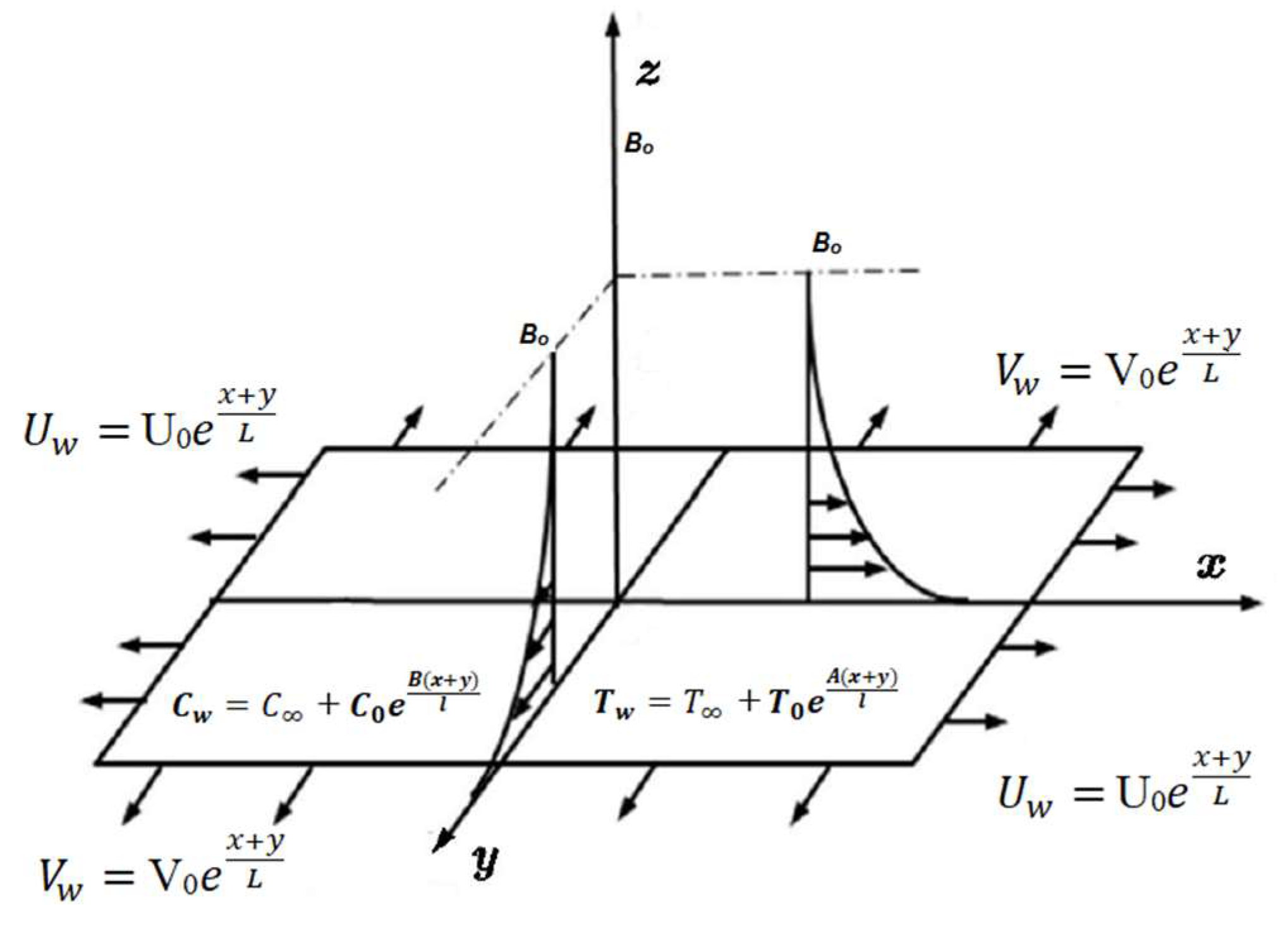
2. Mathematical Modeling
Skin Friction Coefficient and Local Nusselt and Sherwood Numbers
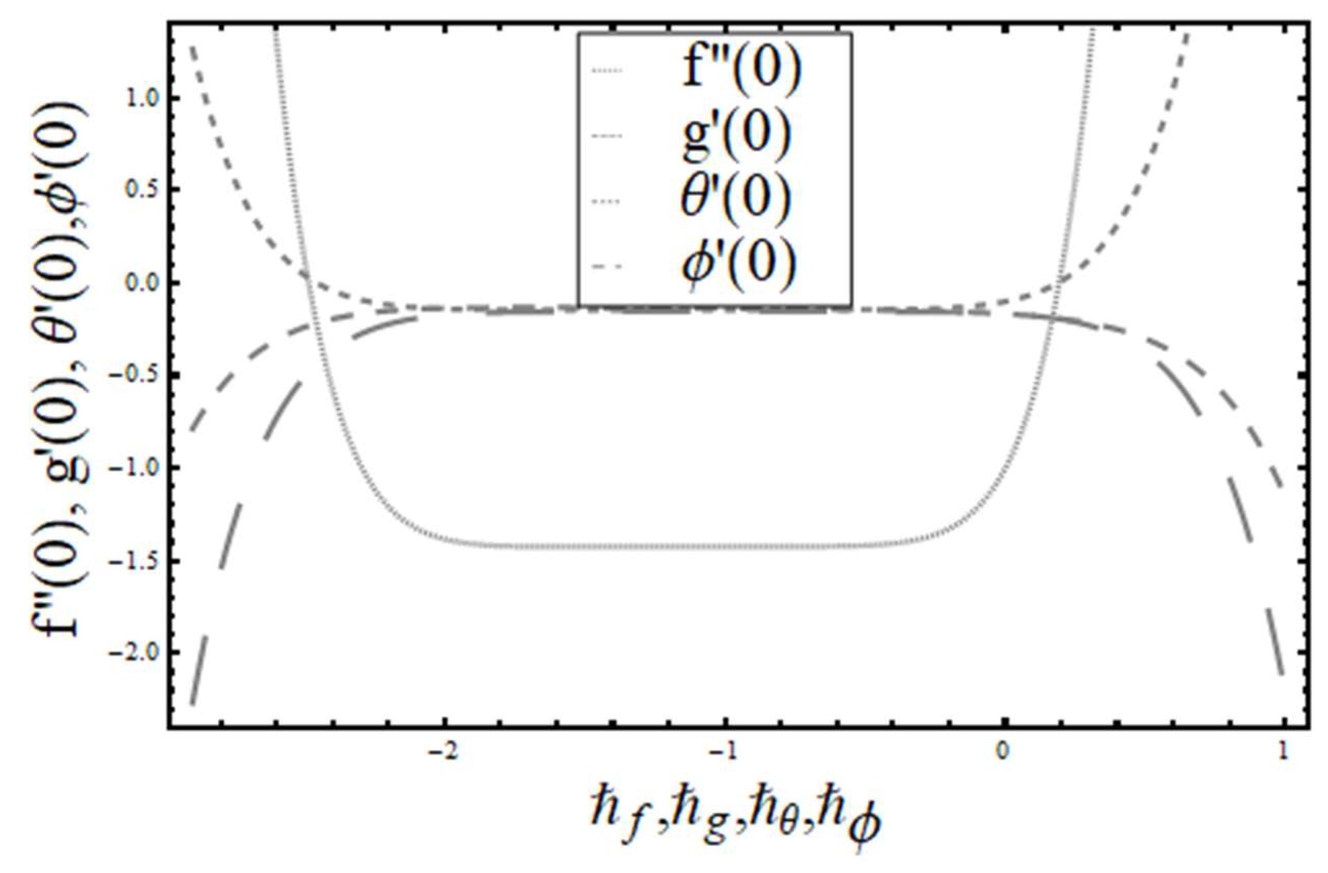
3. Convergence Analysis
3.1. Homotopic Solutions
3.2. Deformation Problems at Zeroth Order
3.3. The m-th Order Problem
4. Entropy Analysis
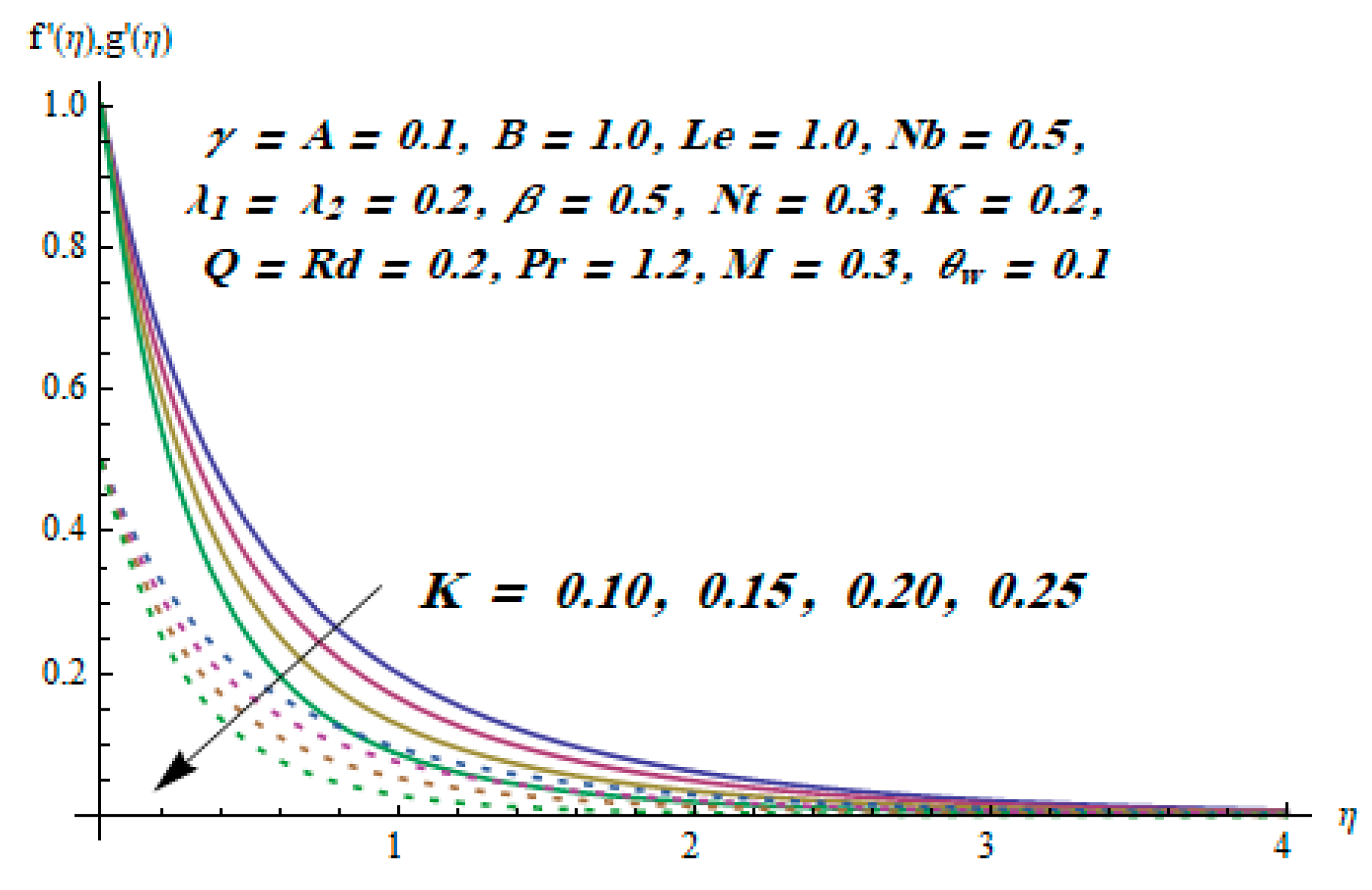
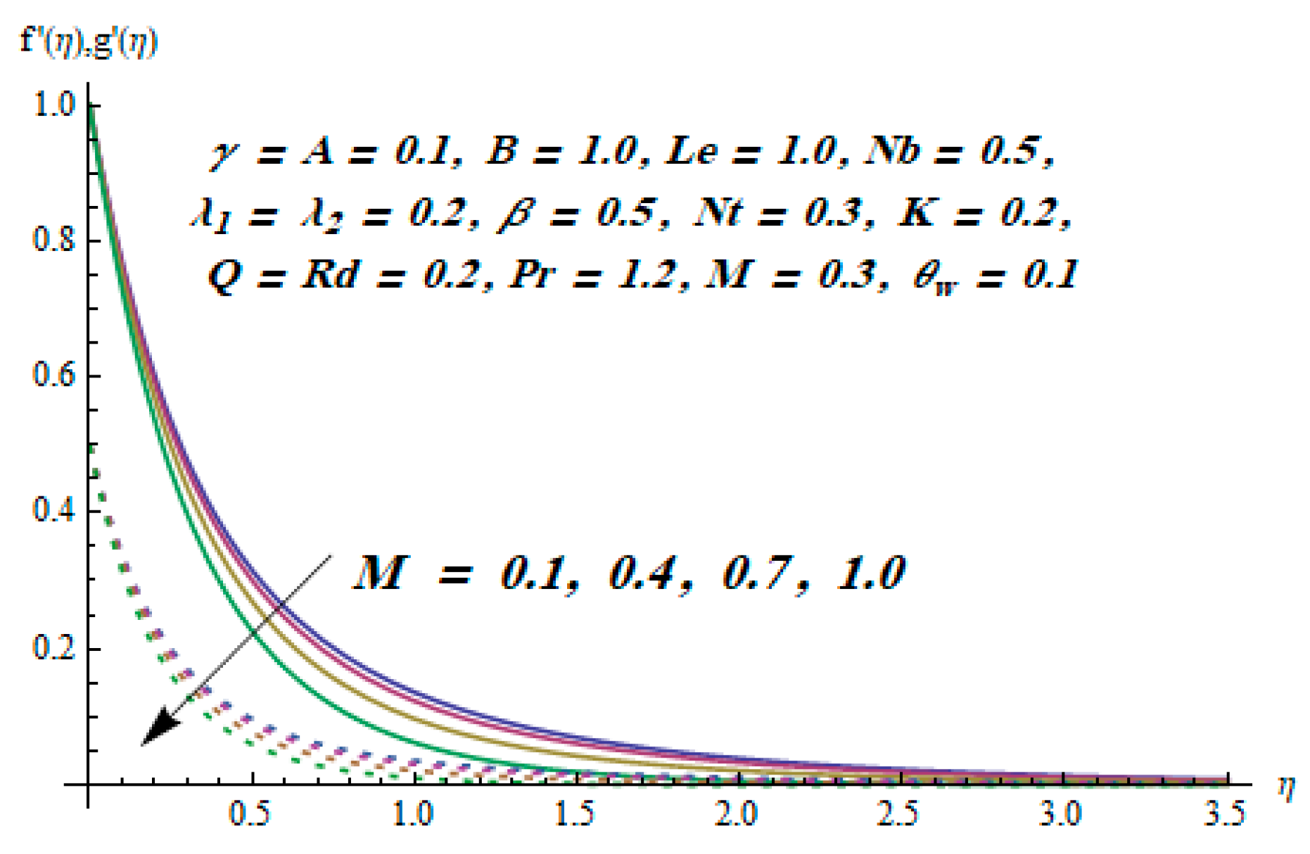
5. Results and Discussion
6. Concluding Remarks
- The velocity components were declining functions of the viscoelastic parameter.
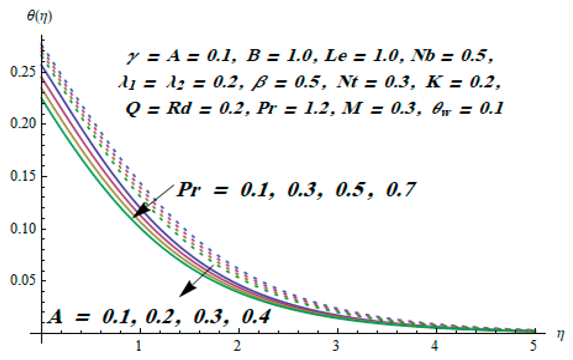
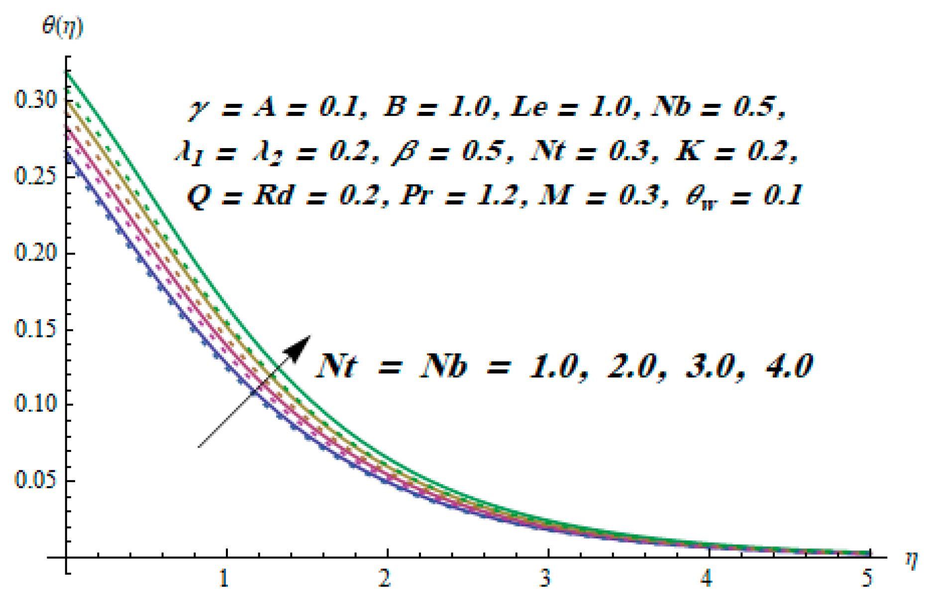
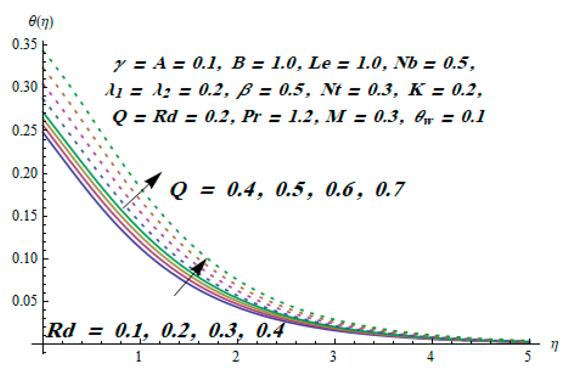
- The temperature field improved with an increase in radiation parameter.
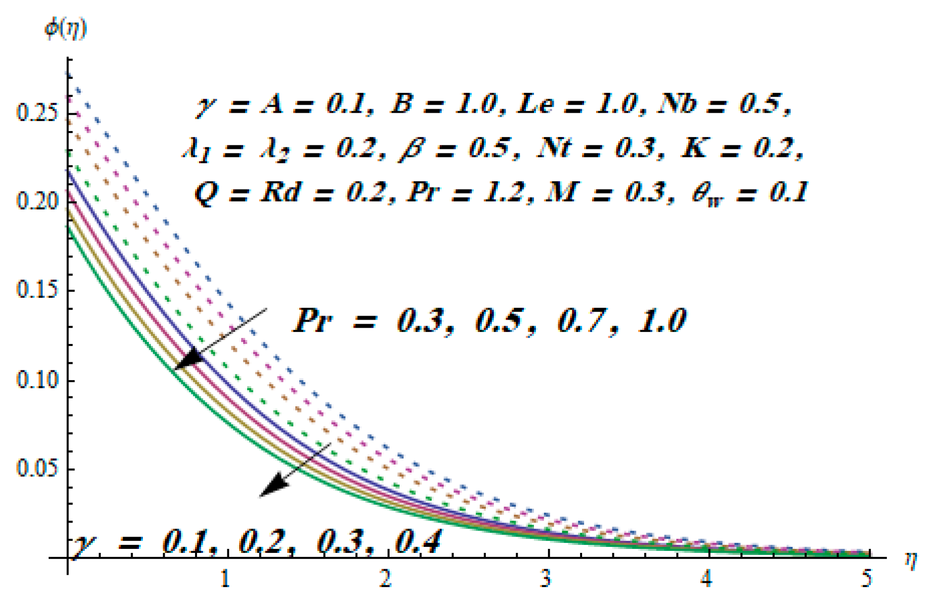
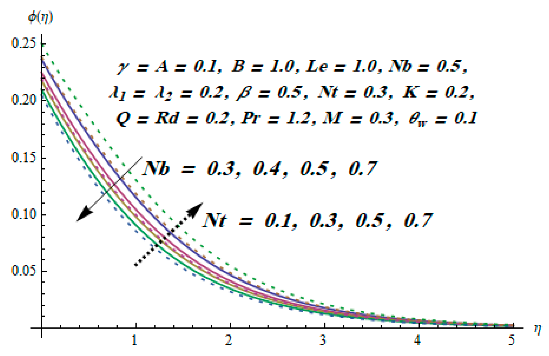
- Thermophoresis and Brownian motion parameters had an opposite effect on concentration distribution.
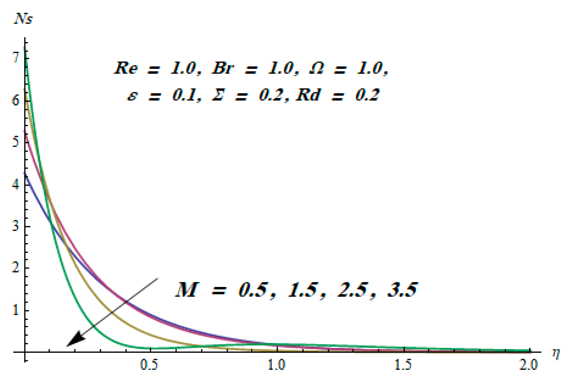
- With growing values of the magnetic parameter, both velocity components declined.
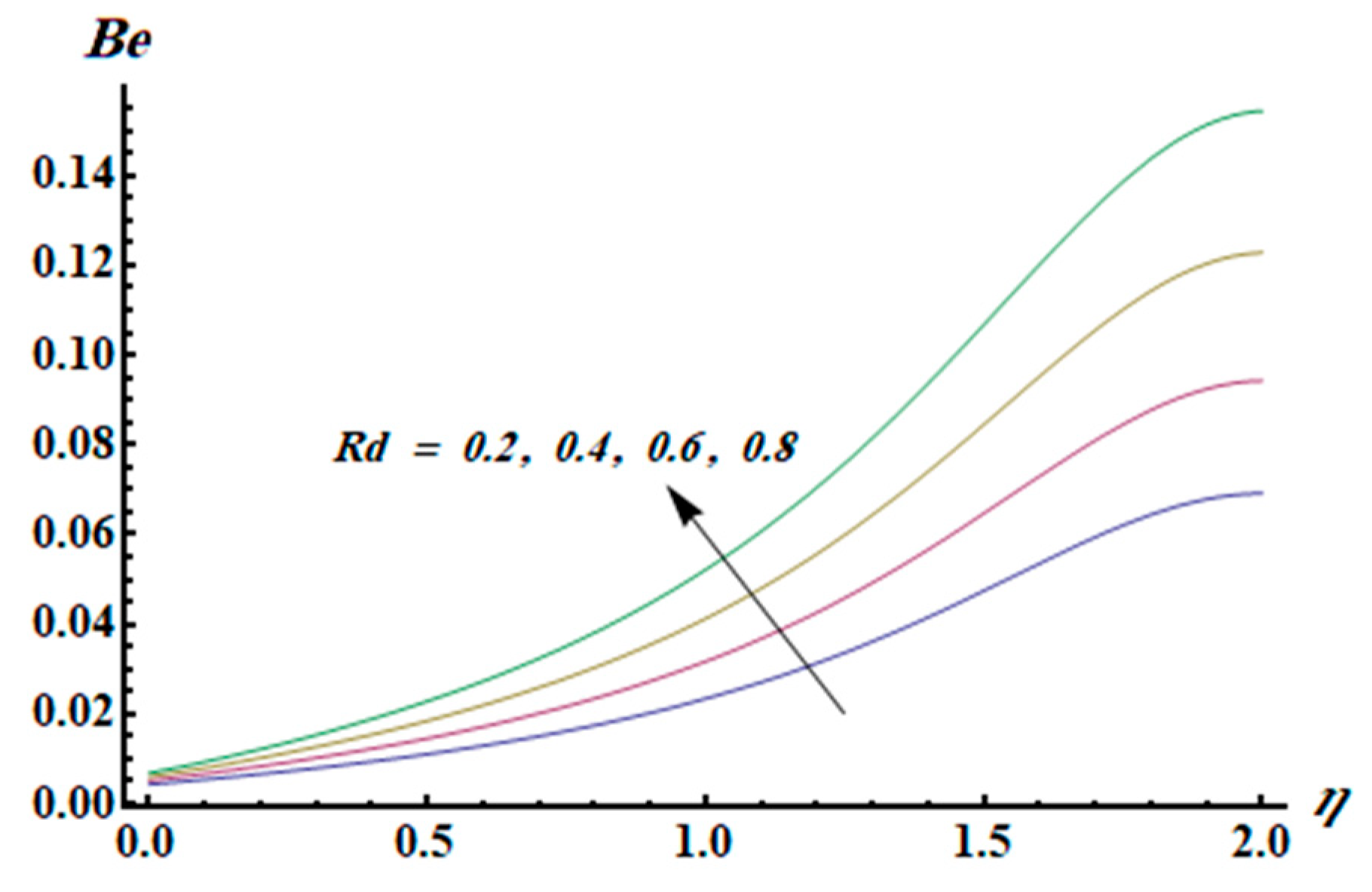
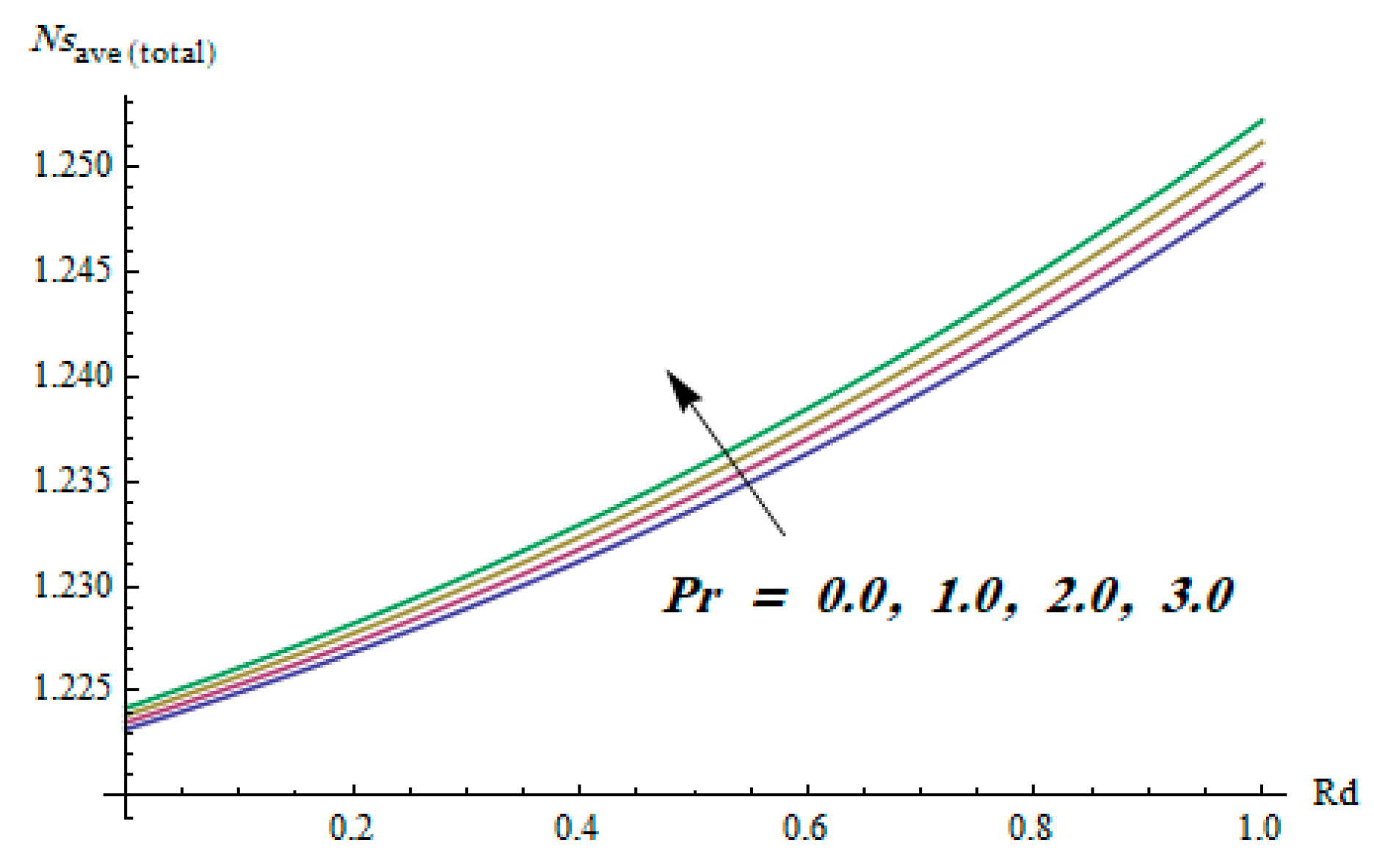
- The Bejan number is an increasing function of the thermal radiation parameter.
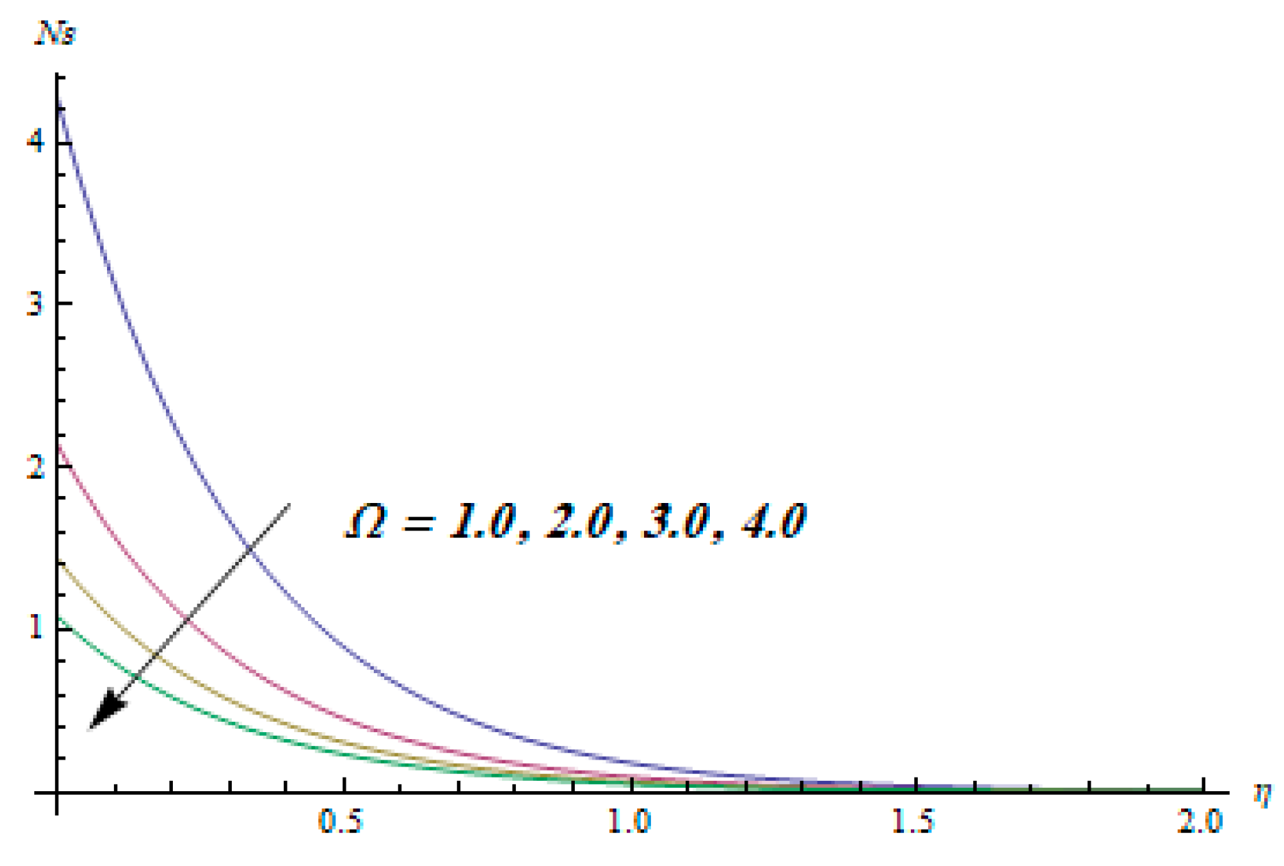
- Entropy generation decreased for escalating values of the temperature difference parameter.
Author Contributions
Funding
Conflicts of Interest
Nomenclature
| a, b, c, d, e | Dimensional constants |
| η | Similarity variable |
| A | Temperature exponent |
| B | Concentration exponent |
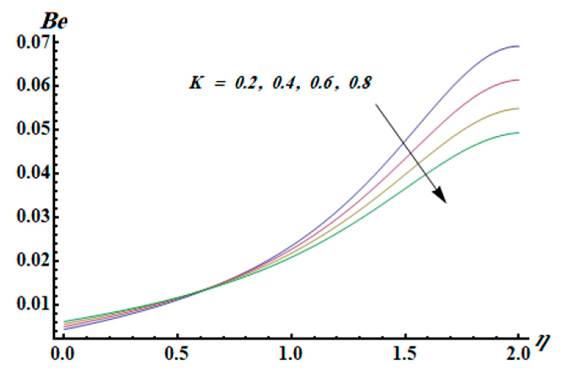
| Be | Bejan number |
| β0 | Magnetic field strength |
| C | Concentration of fluid |
| Cf | Skin friction |
| cp | Specific heat |
| Cw | Concentration on wall |
| C∞ | Ambient concentration |
| C0 | Reference concentration |
| Br | Brinkman number |
| DB | Brownian diffusion coefficient |
| DT | Thermophoretic diffusion coefficient |
| f, g | Dimensionless velocities |
| Effective heat capacity of nanoparticles | |
| k | Thermal conductivity |
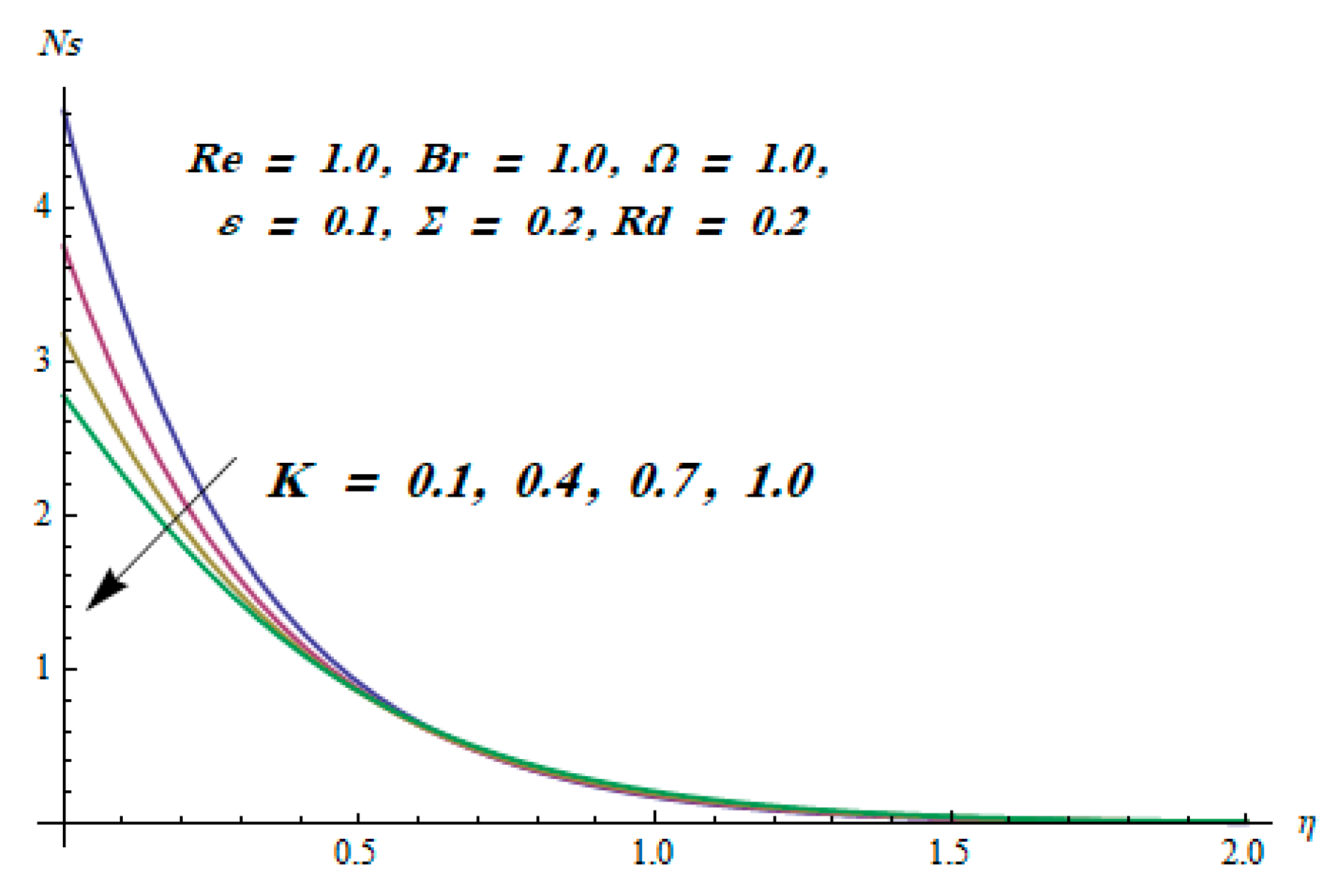
| K | Viscoelastic parameter |
| ko | Elastic parameter |
| K* | Mean absorption coefficient |
| α | Effective heat capacity of fluid |
| Le | Lewis number |
| Nb | Brownian motion parameter |
| Nt | Thermophoresis parameter |
| Nux | Nusselt number |
| M | Magnetic parameter |
| Pr | Prandtl number |
| Q | Heat absorption |
| Rd | Thermal radiation parameter |
| Re | Reynolds number |
| SG | Volumetric entropy generation |
| Nux | Local Nusselt number |
| NS | Entropy generation rate |
| Cfx, Cfy | Skin friction coefficients |
| Shx | Sherwood number |
| T | Temperature of fluid |
| Tw | Wall temperature |
| Constants | |
| T∞ | Ambient temperature |
| Ue | Stretching velocity |
| Uw | Linear stretching velocity |
| (u, v, w) | Velocity components |
| (x, y, z) | Coordinate axes |
| M | Hartmann number |
| Kinematic viscosity | |
| λ1 | Relaxation time |
| Λ2 | Ratio of relaxation to retardation time |
| ρ | Density of fluid |
| σ | Electrical conductivity |
| σ* | Stefan–Boltzmann constant |
| μ | Dynamic viscosity |
| τ | Ratio of nanoparticle |
| τw | Skin friction coefficient |
| Ω | Dimensionless temperature difference |
| ε | Dimensionless nanoparticle volume difference |
| Σ | Nanoparticle mass transfer parameter |
| θ | Dimensionless temperature |
| ϕ | Dimensionless concentration |
| α1 | Normal stress moduli |
| Kc | Chemical reaction coefficient |
| Reference length |
References
- Saidur, R.; Leong, K.Y.; Mohammad, H. A review on applications and challenges of nanofluids. Renew. Sustain. Energy Rev. 2011, 15, 1646–1668. [Google Scholar] [CrossRef]
- Xiao, B.; Zhang, X.; Wang, W.; Long, G.; Chen, H.; Kang, H.; Ren, W. A fractal model for water flow through unsaturated porous rocks. Fractals 2018, 26, 1840015. [Google Scholar] [CrossRef]
- Long, G.; Xu, G. The effects of perforation erosion on practical hydraulic-fracturing applications. SPE J. 2017, 22, 645–659. [Google Scholar] [CrossRef]
- Wong, K.V.; De Leon, O. Applications of nanofluids: Current and future. Adv. Mech. Eng. 2010, 2, 519659. [Google Scholar] [CrossRef]
- Choi, S.U.S.; Estman, J.A. Enhancing thermal conductivity of fluids with nanoparticles. ASME-Publications-Fed 1995, 231, 99–106. [Google Scholar]
- Buongiorno, J. Convective transport in nanofluids. J. Heat Transf. 2006, 128, 240–250. [Google Scholar] [CrossRef]
- Khan, W.A.; Pop, I. Boundary-layer flow of a nanofluid past a stretching sheet. Int. J. Heat Mass Transf. 2010, 53, 2477–2483. [Google Scholar] [CrossRef]
- Makinde, O.D.; Aziz, A. Boundary layer flow of a nanofluid past a stretching sheet with a convective boundary condition. Int. J. Therm. Sci. 2011, 50, 1326–1332. [Google Scholar] [CrossRef]
- Sheikholeslami, M.; Shafee, A.; Ramzan, M.; Li, Z. Investigation of Lorentz forces and radiation impacts on nanofluid treatment in a porous semi annulus via Darcy law. J. Mol. Liquids 2018, 272, 8–14. [Google Scholar] [CrossRef]
- Li, Z.; Sheikholeslami, M.; Shafee, A.; Ramzan, M.; Kandasamy, R.; Al-Mdallal, Q.M. Influence of adding nanoparticles on solidification in a heat storage system considering radiation effect. J. Mol. Liquids 2018, 273, 589–605. [Google Scholar] [CrossRef]
- Muhammad, T.; Lu, D.-C.; Mahanthesh, B.; Eid, M.R.; Ramzan, M.; Dar, A. Significance of Darcy-Forchheimer porous medium in nanofluid through carbon nanotubes. Commun. Theor. Phys. 2018, 70, 361. [Google Scholar] [CrossRef]
- Lu, D.; Ramzan, M.; Ahmad, S.; Chung, J.D.; Farooq, U. A numerical treatment of MHD radiative flow of Micropolar nanofluid with homogeneous-heterogeneous reactions past a nonlinear stretched surface. Sci. Rep. 2018, 8, 12431. [Google Scholar] [CrossRef]
- Ramzan, M.; Ullah, N.; Chung, J.D.; Lu, D.; Farooq, U. Buoyancy effects on the radiative magneto Micropolar nanofluid flow with double stratification, activation energy and binary chemical reaction. Sci. Rep. 2017, 7, 12901. [Google Scholar] [CrossRef] [Green Version]
- Lu, D.C.; Farooq, U.; Hayat, T.; Rashidi, M.M.; Ramzan, M. Computational analysis of three-layer fluid model including a nanomaterial layer. Int. J. Heat Mass Transf. 2018, 122, 222–228. [Google Scholar] [CrossRef]
- Li, Z.; Ramzan, M.; Shafee, A.; Saleem, S.; Al-Mdallal, Q.M.; Chamkha, A.J. Numerical approach for nanofluid transportation due to electric force in a porous enclosure. Microsyst. Technol. 2018, 1–14. [Google Scholar] [CrossRef]
- Liang, M.; Liu, Y.; Xiao, B.; Yang, S.; Wang, Z.; Han, H. An analytical model for the transverse permeability of gas diffusion layer with electrical double layer effects in proton exchange membrane fuel cells. Int. J. Hydrogen Energy 2018, 43, 17880–17888. [Google Scholar] [CrossRef]
- Zhang, D.; Shen, Y.; Zhou, Z.; Qu, J.; Zhou, L.; Wang, J.; Zhang, F. Convection Heat Transfer Performance of Fractal Tube Bank under cross flow. Fractals 2018. [Google Scholar] [CrossRef]
- Xiao, B.; Chen, H.; Xiao, S.; Cai, J. Research on relative permeability of nanofibers with capillary pressure effect by means of fractal-monte carlo technique. J. Nanosci. Nanotechnol. 2017, 17, 6811–6817. [Google Scholar] [CrossRef]
- Sheikholeslami, M. Numerical investigation for CuO-H2O nanofluid flow in a porous channel with magnetic field using mesoscopic method. J. Mol. Liquids 2018, 249, 739–746. [Google Scholar] [CrossRef]
- Lu, D.; Ramzan, M.; ul Huda, N.; Chung, J.D.; Farooq, U. Nonlinear radiation effect on MHD Carreau nanofluid flow over a radially stretching surface with zero mass flux at the surface. Sci. Rep. 2018, 8, 3709. [Google Scholar] [CrossRef]
- Dogonchi, A.S.; Ganji, D.D. Impact of Cattaneo–Christov heat flux on MHD nanofluid flow and heat transfer between parallel plates considering thermal radiation effect. J. Taiwan Inst. Chem. Eng. 2017, 80, 52–63. [Google Scholar] [CrossRef]
- Sheikholeslami, M. Lattice Boltzmann method simulation for MHD non-Darcy nanofluid free convection. Phys. B Condens. Matter 2017, 516, 55–71. [Google Scholar] [CrossRef]
- Ramzan, M.; Bilal, M.; Chung, J.D.; Mann, A.B. On MHD radiative Jeffery nanofluid flow with convective heat and mass boundary conditions. Neural Comput. Appl. 2017, 30, 2739–2748. [Google Scholar] [CrossRef]
- Ramzan, M.; Bilal, M.; Chung, J.D.; Lu, D.C.; Farooq, U. Impact of generalized Fourier’s and Fick’s laws on MHD 3D second grade nanofluid flow with variable thermal conductivity and convective heat and mass conditions. Phys. Fluids 2017, 29, 093102. [Google Scholar] [CrossRef]
- Ramzan, M.; Bilal, M.; Chung, J.D. MHD stagnation point Cattaneo–Christov heat flux in Williamson fluid flow with homogeneous–heterogeneous reactions and convective boundary condition—A numerical approach. J. Mol. Liquids 2017, 225, 856–862. [Google Scholar] [CrossRef]
- Ramzan, M.; Chung, J.D.; Ullah, N. Partial slip effect in the flow of MHD micropolar nanofluid flow due to a rotating disk—A numerical approach. Res. Phys. 2017, 7, 3557–3566. [Google Scholar] [CrossRef]
- Ramzan, M.; Bilal, M.; Chung, J.D. Effects of thermal and solutal stratification on Jeffrey magneto-nanofluid along an inclined stretching cylinder with thermal radiation and heat generation/absorption. Int. J. Mech. Sci. 2017, 131, 317–324. [Google Scholar] [CrossRef]
- Bejan, A. A study of entropy generation in fundamental convective heat transfer. J. Heat Transf. 1979, 101, 718–725. [Google Scholar] [CrossRef]
- Reveillere, A.; Baytas, A.C. Minimum entropy generation for laminar boundary layer flow over a permeable plate. Int. J. Exergy 2010, 7, 164–177. [Google Scholar] [CrossRef]
- López, A.; Ibáñez, G.; Pantoja, J.; Moreira, J.; Lastres, O. Entropy generation analysis of MHD nanofluid flow in a porous vertical microchannel with nonlinear thermal radiation, slip flow and convective-radiative boundary conditions. Int. J. Heat Mass Transf. 2017, 107, 982–994. [Google Scholar] [CrossRef]
- Sheikholeslami, M. New computational approach for exergy and entropy analysis of nanofluid under the impact of Lorentz force through a porous media. Comput. Methods Appl. Mech. Eng. 2018, 344, 319–333. [Google Scholar] [CrossRef]
- Bondareva, N.S.; Sheremet, M.A.; Oztop, H.F.; Abu-Hamdeh, N. Entropy generation due to natural convection of a nanofluid in a partially open triangular cavity. Adv. Powder Technol. 2017, 28, 244–255. [Google Scholar] [CrossRef]
- Sheremet, M.; Pop, I.; Öztop, H.F.; Abu-Hamdeh, N. Natural convection of nanofluid inside a wavy cavity with a non-uniform heating: Entropy generation analysis. Int. J. Numer. Methods Heat Fluid Flow 2017, 27, 958–980. [Google Scholar] [CrossRef]
- Sheremet, M.A.; Grosan, T.; Pop, I. Natural convection and entropy generation in a square cavity with variable temperature side walls filled with a nanofluid: Buongiorno’s mathematical model. Entropy 2017, 19, 337. [Google Scholar] [CrossRef]
- Bhatti, M.M.; Sheikholeslami, M.; Zeeshan, A. Entropy analysis on electro-kinetically modulated peristaltic propulsion of magnetized nanofluid flow through a microchannel. Entropy 2017, 19, 481. [Google Scholar] [CrossRef]
- Farooq, U.; Afridi, M.; Qasim, M.; Lu, D. Transpiration and Viscous Dissipation Effects on Entropy Generation in Hybrid Nanofluid Flow over a Nonlinear Radially Stretching Disk. Entropy 2018, 20, 668. [Google Scholar] [CrossRef]
- Hayat, T.; Aziz, A.; Muhammad, T.; Alsaedi, A. Model and comparative study for flow of viscoelastic nanofluids with Cattaneo-Christov double diffusion. PLoS ONE 2017, 12, e0168824. [Google Scholar] [CrossRef]
- Hayat, T.; Ashraf, B.; Shehzad, S.A.; Alsaedi, A.; Bayomi, N. Three-dimensional mixed convection flow of viscoelastic nanofluid over an exponentially stretching surface. Int. J. Numer. Methods Heat Fluid Flow 2015, 25, 333–357. [Google Scholar] [CrossRef]
- Farooq, M.; Khan, M.I.; Waqas, M.; Hayat, T.; Alsaedi, A.; Khan, M.I. MHD stagnation point flow of viscoelastic nanofluid with non-linear radiation effects. J. Mol. Liquids 2016, 221, 1097–1103. [Google Scholar] [CrossRef]
- Ramzan, M.; Yousaf, F. Boundary layer flow of three-dimensional viscoelastic nanofluid past a bi-directional stretching sheet with Newtonian heating. AIP Adv. 2015, 5, 057132. [Google Scholar] [CrossRef] [Green Version]
- Ramzan, M.; Bilal, M. Three-dimensional flow of an elastico-viscous nanofluid with chemical reaction and magnetic field effects. J. Mol. Liquids 2016, 215, 212–220. [Google Scholar] [CrossRef]
- Ramzan, M.; Inam, S.; Shehzad, S.A. Three dimensional boundary layer flow of a viscoelastic nanofluid with Soret and Dufour effects. Alex. Eng. J. 2016, 55, 311–319. [Google Scholar] [CrossRef]
- Alsaedi, A.; Hayat, T.; Muhammad, T.; Shehzad, S.A. MHD three-dimensional flow of viscoelastic fluid over an exponentially stretching surface with variable thermal conductivity. Comput. Math. Math. Phy. 2016, 56, 1665–1678. [Google Scholar] [CrossRef]
- Mustafa, M.; Ahmad, R.; Hayat, T.; Alsaedi, A. Rotating flow of viscoelastic fluid with nonlinear thermal radiation: A numerical study. Neural Comput. Appl. 2018, 29, 493–499. [Google Scholar] [CrossRef]
- Hayat, T.; Qayyum, S.; Shehzad, S.A.; Alsaedi, A. Cattaneo-Christov double-diffusion theory for three-dimensional flow of viscoelastic nanofluid with the effect of heat generation/absorption. Res. Phys. 2018, 8, 489–495. [Google Scholar] [CrossRef]
- Hayat, T.; Shah, F.; Hussain, Z.; Alsaedi, A. Outcomes of double stratification in Darcy–Forchheimer MHD flow of viscoelastic nanofluid. J. Braz. Soc. Mech. Sci. Eng. 2018, 40, 145. [Google Scholar] [CrossRef]
- Srinivasacharya, D.; Shafeeurrahman, M. Entropy Generation Due to MHD Mixed Convection of Nanofluid Between Two Concentric Cylinders with Radiation and Joule Heating Effects. J. Nanofluids 2017, 6, 1227–1237. [Google Scholar] [CrossRef]
- Noghrehabadi, A.; Saffarian, M.R.; Pourrajab, R.; Ghalambaz, M. Entropy analysis for nanofluid flow over a stretching sheet in the presence of heat generation/absorption and partial slip. J. Mech. Sci. Technol. 2013, 27, 927–937. [Google Scholar] [CrossRef]
- Abelman, S.; Zaib, A. Entropy generation of nanofluid flow over a convectively heated stretching sheet with stagnation point flow having nimonic 80a nanoparticles: Buongiorno model. In Proceedings of the 13th International Conference on Heat Transfer, Fluid Mechanics and Thermodynamics, Portoroz, Slovenia, 17–19 July 2017. [Google Scholar]
- Shit, G.C.; Haldar, R.; Mandal, S. Entropy generation on MHD flow and convective heat transfer in a porous medium of exponentially stretching surface saturated by nanofluids. Adv. Powder Technol. 2017, 28, 1519–1530. [Google Scholar] [CrossRef]
- Turkyilmazoglu, M. Determination of the correct range of physical parameters in the approximate analytical solutions of nonlinear equations using the Adomian decomposition method. Mediterr. J. Math. 2016, 13, 4019–4037. [Google Scholar] [CrossRef]
- Liu, I.-C.; Wang, H.-H.; Peng, Y.-F. Flow and heat transfer for three-dimensional flow over an exponentially stretching surface. Chem. Eng. Commun. 2013, 200, 253–268. [Google Scholar] [CrossRef]


| Order of Approximation | ||||
|---|---|---|---|---|
| 1 | 1.19588 | 0.12037 | 0.16113 | 0.16180 |
| 3 | 1.37115 | 0.13887 | 0.15382 | 0.15745 |
| 7 | 1.42903 | 0.14518 | 0.14911 | 0.15586 |
| 10 | 1.45762 | 0.14852 | 0.14206 | 0.15476 |
| 13 | 1.46000 | 0.14883 | 0.13937 | 0.15471 |
| 14 | 1.46000 | 0.14883 | 0.13798 | 0.15460 |
| 15 | 1.46000 | 0.14883 | 0.13796 | 0.15460 |
| 18 | 1.46000 | 0.14883 | 0.13796 | 0.15460 |
| λ | Nb | Nt | Le | Pr | M | K | Rd | A | Q | ||
|---|---|---|---|---|---|---|---|---|---|---|---|
| 0.1 | - | - | - | - | - | - | - | - | - | 0.13878 | 0.12199 |
| 0.2 | - | - | - | - | - | - | - | - | - | 0.1388 | 0.12157 |
| 0.5 | - | - | - | - | - | - | - | - | - | 0.1421 | 0.12032 |
| - | 0.5 | - | - | - | - | - | - | - | - | 0.13878 | 0.12199 |
| - | 1.0 | - | - | - | - | - | - | - | - | 0.13772 | 0.11917 |
| - | 1.5 | - | - | - | - | - | - | - | - | 0.13770 | 0.11823 |
| - | - | 0.0 | - | - | - | - | - | - | - | 0.13878 | 0.11635 |
| - | - | 0.2 | - | - | - | - | - | - | - | 0.13878 | 0.12199 |
| - | - | 0.5 | - | - | - | - | - | - | - | 0.13878 | 0.12576 |
| - | - | - | 1.0 | - | - | - | - | - | - | 0.14447 | 0.12981 |
| - | - | - | 1.5 | - | - | - | - | - | - | 0.13878 | 0.12199 |
| - | - | - | 2.0 | - | - | - | - | - | - | 0.12572 | 0.11010 |
| - | - | - | - | 1.0 | - | - | - | - | - | 0.13878 | 0.12199 |
| - | - | - | - | 1.2 | - | - | - | - | - | 0.13775 | 0.08889 |
| - | - | - | - | 1.5 | - | - | - | - | - | 0.13774 | 0.06499 |
| - | - | - | - | - | 0.0 | - | - | - | - | 0.13878 | 0.12199 |
| - | - | - | - | - | 0.2 | - | - | - | - | 0.13878 | 0.12199 |
| - | - | - | - | - | 0.3 | - | - | - | - | 0.13878 | 0.12199 |
| - | - | - | - | - | - | 0.0 | - | - | - | 0.13878 | 0.12199 |
| - | - | - | - | - | - | 0.02 | - | - | - | 0.13878 | 0.12199 |
| - | - | - | - | - | - | 0.04 | - | - | - | 0.13878 | 0.12199 |
| - | - | - | - | - | - | - | 0.2 | - | - | 0.13878 | 0.12199 |
| - | - | - | - | - | - | - | 0.4 | - | - | 0.14392 | 0.12146 |
| - | - | - | - | - | - | - | 0.5 | - | - | 0.14480 | 0.12123 |
| - | - | - | - | - | - | - | - | 0.1 | - | 0.13878 | 0.12199 |
| - | - | - | - | - | - | - | - | 0.5 | - | 0.13878 | 0.12199 |
| - | - | - | - | - | - | - | - | 0.7 | - | 0.13878 | 0.12199 |
| - | - | - | - | - | - | - | - | - | 0.2 | 0.13878 | 0.12199 |
| - | - | - | - | - | - | - | - | - | 0.4 | 0.14962 | 0.12199 |
| - | - | - | - | - | - | - | - | - | 0.5 | 0.15679 | 0.12199 |
| λ | M | K | ||
|---|---|---|---|---|
| 0.1 | - | - | 1.6768 | 0.2237 |
| 0.2 | - | - | 1.7698 | 0.4089 |
| 0.5 | - | - | 2.0571 | 1.0804 |
| - | 0.3 | - | 1.6768 | 0.2237 |
| - | 0.5 | - | 1.7422 | 0.2325 |
| - | 1.0 | - | 2.0212 | 0.2697 |
| - | - | 0.02 | 1.6768 | 0.2237 |
| - | - | 0.03 | 1.9607 | 0.2675 |
| - | - | 0.04 | 1.8168 | 0.3138 |
| β | Pr | A | Liu et al. [52] | Present Study |
|---|---|---|---|---|
| 0.0 | 0.7 | 0.0 | −0.42583804 | −0.4258120 |
| 2.0 | −1.02143617 | −1.0214514 | ||
| 5.0 | −1.64165922 | −1.6416620 | ||
| 0.25 | 0.7 | 0.0 | −0.47609996 | −0.4761032 |
| 2.0 | −1.14199997 | −1.1420014 | ||
| 5.0 | −1.83543073 | −1.8354210 | ||
| 0.50 | 0.7 | 0.0 | −0.52154103 | −0.5215267 |
| 2.0 | −1.25099820 | −1.2509991 | ||
| 5.0 | −2.01061361 | −2.0106021 | ||
| 0.75 | 0.7 | 0.0 | −0.56332861 | −0.5633148 |
| 2.0 | −1.35123246 | −1.3512221 | ||
| 5.0 | −2.17171091 | −2.1717006 | ||
| 1.0 | 0.7 | 0.0 | −0.60222359 | −0.6022167 |
| 2.0 | −1.44452826 | −1.4445214 | ||
| 5.0 | −2.32165661 | −2.3216340 |
© 2018 by the authors. Licensee MDPI, Basel, Switzerland. This article is an open access article distributed under the terms and conditions of the Creative Commons Attribution (CC BY) license (http://creativecommons.org/licenses/by/4.0/).
Share and Cite
Suleman, M.; Ramzan, M.; Zulfiqar, M.; Bilal, M.; Shafee, A.; Chung, J.D.; Lu, D.; Farooq, U. Entropy Analysis of 3D Non-Newtonian MHD Nanofluid Flow with Nonlinear Thermal Radiation Past over Exponential Stretched Surface. Entropy 2018, 20, 930. https://0-doi-org.brum.beds.ac.uk/10.3390/e20120930
Suleman M, Ramzan M, Zulfiqar M, Bilal M, Shafee A, Chung JD, Lu D, Farooq U. Entropy Analysis of 3D Non-Newtonian MHD Nanofluid Flow with Nonlinear Thermal Radiation Past over Exponential Stretched Surface. Entropy. 2018; 20(12):930. https://0-doi-org.brum.beds.ac.uk/10.3390/e20120930
Chicago/Turabian StyleSuleman, Muhammad, Muhammad Ramzan, Madiha Zulfiqar, Muhammad Bilal, Ahmad Shafee, Jae Dong Chung, Dianchen Lu, and Umer Farooq. 2018. "Entropy Analysis of 3D Non-Newtonian MHD Nanofluid Flow with Nonlinear Thermal Radiation Past over Exponential Stretched Surface" Entropy 20, no. 12: 930. https://0-doi-org.brum.beds.ac.uk/10.3390/e20120930