Semi-Supervised Minimum Error Entropy Principle with Distributed Method

Abstract

The minimum error entropy principle (MEE) is an alternative of the classical least squares for its robustness to non-Gaussian noise. This paper studies the gradient descent algorithm for MEE with a semi-supervised approach and distributed method, and shows that using the additional information of unlabeled data can enhance the learning ability of the distributed MEE algorithm. Our result proves that the mean squared error of the distributed gradient descent MEE algorithm can be minimax optimal for regression if the number of local machines increases polynomially as the total datasize.

1. Introduction

The minimum error entropy (MEE) principle is an important criterion proposed in information theoretical learning (ITL) [1] and was firstly addressed for adaptive system training by Erdogmus and Principe [2]. It has been applied to blind source separation, maximally informative subspace projections, clustering, feature selection, blind deconvolution, minimum cross-entropy for model selection, and some other topics [3,4,5,6,7,8]. Taking entropy as a measure of the error, the MEE principle can extract the information contained in data fully and produce robustness to outliers in the implementation of algorithms.

Let $X\in {\mathcal{R}}^n$ be an explanatory variable with values taken in a compact metric space $(\mathcal{X},d),$Y be a real response variable with $Y\in \mathcal{Y}\subset \mathcal{R}$, and $g:\mathcal{X}\to \mathcal{Y}$ be a prediction function. For a given set of labeled examples $D={\left\{(x_i,y_i)\right\}}_{i=1}^N\subset \mathcal{X}\times \mathcal{Y}$ (N denotes the sample size) and a windowing function $G:\mathbb{R}\to {\mathbb{R}}_{+},$ the MEE principle is to find a minimizer of the empirical quadratic entropy:

$$\begin{array}{c}\hfill {\displaystyle \widehat{H}\left(g\right)=-log\left\{\frac{h^2}{N^2}\sum _{\begin{array}{c}(x_i,y_i)\in D\\ (x_j,y_j)\in D\end{array}}G\left(\frac{{[(y_i-g\left(x_i\right))-(y_j-g\left(x_j\right))]}^2}{h^2}\right)\right\},}\end{array}$$

where $h>0$ is the scaling parameter. Its goal is to solve the problem $y=g_{\rho }\left(x\right)+\epsilon$, where $\epsilon$ is the noise and $g_{\rho }\left(x\right)$ is the target function. Taking a function $f(x_i,x_j):=g\left(x_i\right)-g\left(x_j\right),$ MEE belongs to pairwise learning problems, which involves with the intersections of example pairs. Since logarithmic function is monotonic, we only consider the empirical information error of MEE:

$$\begin{array}{c}\hfill {\displaystyle R\left(f\right)=-\frac{h^2}{N^2}\sum _{\begin{array}{c}(x_i,y_i)\in D\\ (x_j,y_j)\in D\end{array}}G\left(\frac{{[y_i-y_j-f(x_i,x_j)]}^2}{h^2}\right),}\end{array}$$

(1)

in the optimization process. Borrowing the idea from Reference [9], we introduced the Mercer kernel $K(·,·):{\mathcal{X}}^2\times {\mathcal{X}}^2\to \mathbb{R},({\mathcal{X}}^2:=\mathcal{X}\times \mathcal{X})$ and employed the reproducing kernel Hilbert space (RKHS) ${\mathcal{H}}_K$ as our hypothesis space. With $K,$ ${\mathcal{H}}_K$ is defined as the linear span of the functions set $\{K_{(x,u)}:=K\left((x,u),(·,·)\right),\forall (x,u)\in {\mathcal{X}}^2\},$ which is equipped with the inner product ${\langle ·,·\rangle }_K$ and the reproducing property ${\langle K_{(x,u)},K_{(x^{\prime },u^{\prime })}\rangle }_K=K((x,u),(x^{\prime },u^{\prime })),\forall (x,u),(x^{\prime },u^{\prime })\in {\mathcal{X}}^2.$ For the G nonconvex, we usually solve Equation (1) using the kernel-based gradient descent method as follows. It starts with $f_{1,D}=0$ and is updated by:

$$\begin{array}{c}\hfill f_{t+1,D}=f_{t,D}-\eta \times \nabla \mathcal{R}\left(f_{t,D}\right),\end{array}$$

(2)

in the t-th step, where $\eta >0$ is a step size, ∇ is the gradient operator and:

$${\displaystyle \nabla \mathcal{R}\left(f_{t,D}\right)=-\frac{1}{N^2}\sum _{\begin{array}{c}(x_i,y_i)\in D\\ (x_j,y_j)\in D\end{array}}{G}^{\prime }\left(\frac{{[y_i-y_j-f_{t,D}(x_i,x_j)]}^2}{h^2}\right)[f_{t,D}(x_i,x_j)-y_i+y_j]K_{(x_i,x_j)},}$$

as we know that the example pairs will grow quadratically with the increasing example size N, which will bring the computational burden in the MEE implementation. Thus, it is necessary to reduce the algorithmic complexity by the distributed method based on a divide-and-conquer strategy [10]. Semi-supervised learning (SSL) [11] has attracted extensive attention as an emerging field in machine learning research and data mining. Actually, in many practical problems, few data are given, but a large number of unlabeled data are available, since labeling data requires a lot of time, effort or money. In this paper, we study a distributed MEE algorithm in the framework of SSL and show that the learning ability of the MEE algorithm can be enhanced by the distributed method and the combination of labeled data with unlabeled data.

There are mainly three contributions in this paper. The first one is that we derive the explicit learning rate of the gradient descent method for distributed MEE in the context of SSL, which is comparable to the minimax optimal rate of the least squares in regression. This implies that the MEE algorithm can be an alternative of the least squares in SSL in the sense that both of them have the same prediction power. The second one is that we provide the theoretical upper bound for the number of local machines guaranteeing the optimal rate in the distributed computation. The last one is that we extend the range of the target function allowed in the distributed MEE algorithm.

In

Table 1. List of notations used throughout the paper.

Notation	Meaning of the Notation
X	the explanatory variable
Y	the response variable
$\mathcal{X}$	$X\in \mathcal{X}$, a compact subset of an Euclidian space ${\mathbb{R}}^n$
$\mathcal{Y}$	$Y\in \mathcal{Y}$, a subset of $\mathbb{R}$
$\rho (·,·)$	a Boreal measure on $\mathcal{X}\times \mathcal{Y}$
${\rho }_{\mathcal{X}}$	the marginal probability measure of $\rho$ on $\mathcal{X}$
$\rho (y|x)$	the conditional probability measure of $y\in \mathcal{Y}$ given $X=x$
$g_{\rho }\left(x\right)$	the mean regression function $g_{\rho }\left(x\right)={\int }_{\mathcal{Y}}yd\rho (y|x)$
$f_{\rho }(x,u)$	the target function of MEE induced by $f_{\rho }(x,u)=g_{\rho }\left(x\right)-g_{\rho }\left(u\right)$
K	a reproducing kernel on $\mathcal{X}\times \mathcal{X}$
D	the labeled data set $D=\{(x_1,y_1),\dots ,(x_N,y_N)\}$
N	the size of labeled data set D
$\lceil N/4\rceil$	the largest integer not exceeding $N/4$
$|D|$	the cardinality of $D,$ $|D|=N$
$D^{*}$	the unlabeled data set $D^{*}=\{x_1,\dots ,x_S\}$
S	the size of unlabeled data set $D^{*}$
$|D^{*}|$	the cardinality of $D^{*},$ $|D^{*}|=S$
$\tilde{D}$	training data set used in the distributed MEE algorithm, consisting of D and $D^{*}$
$|\tilde{D}|$	the cardinality of $\tilde{D},$ $|\tilde{D}|=N+S$
m	the number of local machines
${\tilde{D}}_l$	the lth subset of $\tilde{D},$ $1\le l\le m$
G	the loss function of MEE algorithm
$L_K$	the integral operator associated with K
$L_{K,\tilde{D}}$	the empirical operator of $L_K$ on $\tilde{D}$
$f_{t+1,D}$	the function output by the kernel gradient descent MEE algorithm
	with data D and kernel K after t iterations
$f_{t+1,D_l}$	the function output by the kernel gradient MEE algorithm
	with data $D_l$ and kernel K after t iterations
${\overline{f}}_{t+1,\tilde{D}}$	the global output averaging over local outputs $f_{t+1,{\tilde{D}}_l},l=1,\dots ,m$

, we summarize some notations used in this paper.

2. Algorithms and Main Results

We considered MEE for the regression problem. To allow noise in sampling processes, we assumed that a Borel measure $\rho (·,·)$ is defined on the product space $\mathcal{X}\times \mathcal{Y}.$ Let $\rho (y|x)$ be the conditional distribution of $y\in \mathcal{Y}$ for any given $x\in \mathcal{X}$, and ${\rho }_{\mathcal{X}}(·)$ the marginal distribution on $\mathcal{X}.$ For the semi-supervised MEE algorithm, our goal was to estimate the regression function $g_{\rho }\left(x\right)={\int }_{\mathcal{Y}}yd\rho (y|x),x\in \mathcal{X}$, from labeled examples $D={\left\{(x_i,y_i)\right\}}_{i=1}^N$ and unlabeled examples $D^{*}={\left\{x_j\right\}}_{j=1}^S$ drawn from the distribution $\rho$ and ${\rho }_{\mathcal{X}}$, respectively.

Based on the divide-and-conquer strategy, both D and $D^{*}$ are partitioned equally into m subsets, $D={\sum }_{l=1}^m\bigcup D_l$ and $D^{*}={\sum }_{l=1}^m\bigcup D_l^{*}.$ Here, we denote the size of subsets $|D_l|=n$ and $|D_l^{*}|=s$, $1\le l\le m,$ i.e., $N=mn,S=ms.$ We construct a new dataset $\tilde{D}={\sum }_{l=1}^m\bigcup {\tilde{D}}_l$ by:

$$\begin{array}{c}\hfill {\tilde{D}}_l=D_l\cup D_l^{*}={\left\{(x_k,y_k)\right\}}_{k=1}^{n+s},\end{array}$$

where:

$$x_k=\left\{\begin{array}{cc}{x}_k,\hfill & \mathrm{if}(x_k,y_k)\in D_l,\hfill \\ x_k,\hfill & \mathrm{if}{x}_k\in D_l^{*},\hfill \end{array}\right.\mathrm{and}{y}_k=\left\{\begin{array}{cc}\frac{n+s}{n}{y}_k,\hfill & \mathrm{if}(x_k,y_k)\in D_l,\hfill \\ 0,\hfill & \mathrm{if}{x}_k\in D_l^{*}.\hfill \end{array}\right.$$

Based on the gradient descent algorithm (Equation (2)), we can get a set of local estimators $\left\{f_{t,{\tilde{D}}_l}\right\}$ for each subset ${\tilde{D}}_l,1\le l\le m.$ Then, the global estimator averaging over these local estimators is given by:

$$\begin{array}{c}\hfill {\overline{f}}_{t,\tilde{D}}=\frac{1}{m}\sum _{l=1}^m{f}_{t,{\tilde{D}}_l}.\end{array}$$

(3)

In the pairwise setting, our target function $f_{\rho }(x,x^{\prime })=g_{\rho }\left(x\right)-g_{\rho }\left(x^{\prime }\right),x,x^{\prime }\in \mathcal{X},$ which is the difference of the regression function $g_{\rho }.$ Denote by $L_{{\rho }_{{\mathcal{X}}^2}}^2$ the space of square integrable functions on the product space ${\mathcal{X}}^2$:

$$\begin{array}{c}\hfill L_{{\rho }_{{\mathcal{X}}^2}}^2:=\left\{f:{\mathcal{X}}^2\to \mathcal{R}:{\parallel f\parallel }_{L^2}={\left(\int {\int }_{{\mathcal{X}}^2}{|f(x,x^{\prime })|}^{2}d{\rho }_{\mathcal{X}}\left(x\right)d{\rho }_{\mathcal{X}}\left(x^{\prime }\right)\right)}^{\frac{1}{2}}<\infty \right\}.\end{array}$$

The goodness of ${\overline{f}}_{t,\tilde{D}}$ is usually measured by the mean squared error $\parallel {\overline{f}}_{t,\tilde{D}}-f_{\rho }{\parallel }_{L^2}^2.$

Throughout the paper, we assumed that ${\displaystyle \underset{(x,x^{\prime })\in {\mathcal{X}}^2}{sup}\sqrt{K((x,x^{\prime }),(x,x^{\prime }))}\le 1}$ and for some constant $M>0,$ $|y|\le M$ almost surely. Without generality, windowing function G is assumed to be differentiable and satisfies $G^{\prime }\left(0\right)=-1,$ $G^{\prime }\left(u\right)<0$ for $u>0,$ $C_G:={sup}_{u\in (0,\infty )}|G^{\prime }\left(u\right)|<\infty$ and there exists some p such that $c_p>0$ and:

$$\begin{array}{c}\hfill |G^{\prime }\left(u\right)-G^{\prime }\left(0\right)|\le c_p{|u|}^p,\forall u>0.\end{array}$$

(4)

It is easy to check that the Gaussian kernel $G\left(u\right)=exp\{-u\}$ satisfies the assumptions above with $p=1.$

Before we present our main results, define an integral operator $L_K:L_{{\rho }_{{\mathcal{X}}^2}}^2⟶L_{{\rho }_{{\mathcal{X}}^2}}^2$ associated with the kernel K by:

$$\begin{array}{c}\hfill L_K\left(f\right):={\int }_{\mathcal{X}}{\int }_{\mathcal{X}}f(x,x^{\prime })K_{(x,x^{\prime })}d{\rho }_{\mathcal{X}}\left(x\right)d{\rho }_{\mathcal{X}}\left(x^{\prime }\right),\forall f\in L_{{\rho }_{{\mathcal{X}}^2}}^2.\end{array}$$

Our error analysis for the distributed MEE algorithm (Equation (3)) is stated in terms of the following regularity condition:

$$\begin{array}{c}\hfill f_{\rho }=L_K^r\left(\varphi \right)forsomer>0,\varphi \in L_{{\rho }_{{\mathcal{X}}^2}}^2,\end{array}$$

(5)

where $L_K^r$ denotes the r-th power of $L_K$ on $L_{{\rho }_{{\mathcal{X}}^2}}^2$ and is well defined, since the operator $L_K$ is positive and compact with the Mercer kernel $K.$ We use the effective dimension [12,13] $\mathcal{N}\left(\lambda \right)$ to measure the complexity of ${\mathcal{H}}_K$ with respect to ${\rho }_{\mathcal{X}},$ which is defined to be the trace of the operator ${(\lambda I+L_K)}^{-1}{L}_K$ as:

$$\begin{array}{c}\hfill \mathcal{N}\left(\lambda \right)=Tr\left({(\lambda I+L_K)}^{-1}{L}_K\right),\lambda >0.\end{array}$$

To obtain optimal learning rates, we need to quantify $\mathcal{N}\left(\lambda \right)$ of ${\mathcal{H}}_K$. A suitable assumption is: that

$$\begin{array}{c}\hfill \mathcal{N}\left(\lambda \right)\le C_0{\lambda }^{-\beta },forsome{C}_0>0and0<\beta \le 1.\end{array}$$

(6)

Remark 1.

When $\beta =1,$ Equation (6) always holds with $C_0=Tr\left(L_K\right).$ For $0<\beta <1,$ when ${\mathcal{H}}_K$ is a Sobolev space $W^{\alpha }\left(\mathcal{X}\right)$ on $\mathcal{X}\subset {\mathcal{R}}^d$ with all derivative of order up to $\alpha >\frac{d}{2},$ then Equation (6) is satisfied with $\beta =\frac{d}{2\alpha }$ [14]. Moreover, if the eigenvalues ${\left\{{\gamma }_i\right\}}_{i=1}^{\infty }$ of the operator $L_K$ decays as ${\gamma }_i=O\left(i^{-b}\right)$ for some $b>1,$ then $\mathcal{N}\left(\lambda \right)=O\left({\lambda }^{-\frac{1}{b}}\right).$ The eigenvalues assumption is typical in the analysis of the performances of kernel methods estimators and recently used in References [13,15,16] to establish the optimal learning rate in the least square problems.

The following theorem shows that the distributed gradient descent algorithm (Equation (3)) can achieve the optimal rate by providing the iteration time T and the maximal number of local machines, whose proof can be found in Section 3.

Theorem 1. (Main Result)

Assume Equations (5) and (6) hold for$r+\beta \ge \frac{1}{2}.$Let the iteration time$T={\lceil N/4\rceil }^{\frac{1}{2r+\beta }}$and$S+N\ge N^{\frac{\beta +1}{2r+\beta }}$:

$$\begin{array}{c}\hfill m<\frac{min\{{(N+S)}^{\frac{1}{2}}{N}^{-\frac{\beta +1}{4r+2\beta }},{(N+S)}^{\frac{1}{3}}{N}^{-\frac{2-2r-\beta }{6r+3\beta }}\}}{{log}^{6}N},\end{array}$$

(7)

then for any $0<\delta <1,$ with confidence at least $1-\delta$:

$$\begin{array}{c}\hfill \parallel {\overline{f}}_{T+1,\tilde{D}}-f_{\rho }{\parallel }_{L^2}\le C^{\prime }max\left\{N^{-\frac{r}{2r+\beta }},h^{-2p}{(N+S)}^{2p+1}{N}^{\frac{p+\frac{3}{2}}{2r+\beta }-(2p+1)}\right\}{log}^4\frac{24}{\delta },\end{array}$$

(8)

where $C^{\prime }$ is a constant independent of $N,S,\delta ,h$ and $\lceil N/4\rceil$ denotes the largest number not exceeding $N/4.$

Corollary 1.

Under the same conditions of Theorem 1, if the scaling parameter:

$$\begin{array}{c}\hfill h>{(N+S)}^{\frac{2p+1}{2p}}{N}^{\frac{r+p+\frac{3}{2}}{2p(2r+\beta )}}{N}^{-\frac{2p+1}{2p}},\end{array}$$

then for any $0<\delta <1,$ with confidence at least $1-\delta$:

$$\begin{array}{c}\hfill \parallel {\overline{f}}_{T+1,\tilde{D}}-f_{\rho }{\parallel }_{L^2}\le C^{\prime }{N}^{-\frac{r}{2r+\beta }}{log}^4\frac{24}{\delta }.\end{array}$$

(9)

Remark 2.

The rate $O\left(N^{-\frac{r}{2r+\beta }}\right)$ in Equation (9) is optimal in the minimax sense for kernel regression problems [13]. When $m=1,$ the result of Equation (9) shows that the kernel gradient descent MEE algorithm (Equation (2)) on a single big data set can achieve the minimax optimal rate for regression. Thus, MEE is a nice alternative of the classical least squares. Meanwhile, the upper bound (Equation (7)) for the number of local machines implies that the performance of the distributed MEE algorithm (Equation (3)) can be as good as the standard MEE algorithm (2) (acting on the whole data set $\tilde{D}$), provided that the subset ${\tilde{D}}_l$’s size $n+s$ is not too small.

Remark 3.

If no unlabeled data is engaged in the algorithm (Equation (3)), then $S=0$ and the upper bound (Equation (7)) for the number of local machines m that ensures the optimal rate is about $O\left(N^{\frac{r-\frac{1}{2}}{2r+\beta }}\right).$ So, when the regularity parameter r in Equation (5) is close to $\frac{1}{2},$ the upper bound $O\left(N^{\frac{r-\frac{1}{2}}{2r+\beta }}\right)$ reduces to a constant and then the distributed algorithm (Equation (3)) will not be feasible in real applications. A similar phenomenon is observed in various distributed algorithms [15,16,17,18]. When the size of unlabeled data $S>0,$ we see from Equation (7) that the upper bound of m keeps growing with the increase of S when the size of labeled data N is fixed. For example, let $\beta >\frac{1}{2}$ and $S=N^{\frac{1}{2r+\beta }}$, then the upper bound in Equation (7) is $O\left(N^{\frac{r}{2r+\beta }}\right)$ and will not be a constant when $r\to \frac{1}{2}.$ Hence, with sufficient unlabeled data $D^{*}$, the distributed algorithm (Equation (3)) will allow more local machines in the distributed method.

Remark 4.

A series of distributed works [15,16,17,18,19] were carried out when the target function $f_{\rho }$ lies in the space ${\mathcal{H}}_K,$ i.e., the regularization parameter $r>\frac{1}{2}.$ As a byproduct, our work in Theorem 1 does not impose the restriction $r>\frac{1}{2}$ on the distributed algorithm (Equation (3)).

3. Proof of Main Result

In this section we prove our main results in Theorem 1. To this end, we introduce the data-free gradient descent method in ${\mathcal{H}}_K$ for the least squares, defined as $f_1=0$ and:

$$\begin{array}{c}\hfill f_{t+1}=f_t-{\eta }_t{\int }_{\mathcal{X}}{\int }_{\mathcal{X}}(f_t(x,x^{\prime })-f_{\rho }(x,x^{\prime }))K_{(x,x^{\prime })}d{\rho }_{\mathcal{X}}\left(x\right)d{\rho }_{\mathcal{X}}\left(x^{\prime }\right),t\ge 1.\end{array}$$

Recalling the definition of $L_K$, it can be written as:

$$\begin{array}{c}\hfill f_{t+1}=f_t-{\eta }_t{L}_K(f_t-f_{\rho })=(I-{\eta }_t{L}_K)f_t+{\eta }_t{L}_K\left(f_{\rho }\right),t\ge 1.\end{array}$$

(10)

Following the standard decomposition technique in leaning theory, we split the error ${\overline{f}}_{t+1,\tilde{D}}-f_{\rho }$ into the sample error ${\overline{f}}_{t+1,\tilde{D}}-f_{t+1}$ and the approximation error $f_{t+1}-f_{\rho }.$

3.1. Approximation Error

Firstly, we estimate the approximation error $\parallel f_{t+1}-f_{\rho }{\parallel }_{L^2}.$ It has been proven in Reference [20] and shown in the lemmas as follows.

Lemma 1.

Define $\left\{f_t\right\}$ by Equation (10) with $0<\eta \le 1.$ If Equation (5) holds with $r>0$, there are:

$$\begin{array}{c}\hfill \parallel f_t-f_{\rho }{\parallel }_{L^2}\le c_{\varphi ,r}{t}^{-r},\end{array}$$

and when $r\ge \frac{1}{2}$:

$$\begin{array}{c}\hfill \parallel f_t-f_{\rho }{\parallel }_K\le c_{\varphi ,r}{t}^{-(r-\frac{1}{2})},\end{array}$$

where $c_{\varphi ,r}=max\left\{{\parallel \varphi \parallel }_{L^2}{(2r/e)}^r,{\parallel \varphi \parallel }_{L^2}{[(2r-1)/e]}^{r-\frac{1}{2}}\right\}$.

Moreover, we derive the uniform bound of the sequence $\left\{f_t\right\}$ by Equation (10) when $0<r<\frac{1}{2}$, which is useful in our analysis. Here and in the sequel, denote ${\pi }_{i+1}^t\left(L\right)$ as the polynomial operator associated with an operator L defined by ${\pi }_{i+1}^t\left(L\right):={\prod }_{j=i+1}^t(I-\eta L)$ and ${\pi }_{t+1}^t:=I.$ We use the conventional notation ${\sum }_{j=T+1}^T:=1.$

Lemma 2.

Define $\left\{f_t\right\}$ by Equation (10) with $0<\eta \le 1.$ If Equation (5) holds with $0<r<\frac{1}{2}$, there are:

$$\begin{array}{c}\hfill \parallel f_t{\parallel }_K\le d_{\varphi ,\eta ,r}{t}^{\frac{1}{2}-r},\end{array}$$

(11)

where $d_{\varphi ,\eta ,r}$ is defined in the proof.

Proof. 

Using Equation (10) iteratively from t to $1,$ then we have that:

$$\begin{array}{c}\hfill f_{t+1}=\sum _{i=1}^t\eta {\pi }_{i+1}^t\left(L_K\right)L_K\left(f_{\rho }\right),forallt\ge 1.\end{array}$$

With Equation (5):

$$\begin{array}{cc}\hfill \parallel f_{t+1}{\parallel }_K& ={∥\sum _{i=1}^t\eta {\pi }_{i+1}^t\left(L_K\right)L_K\left(f_{\rho }\right)∥}_K={∥\sum _{i=1}^t\eta {\pi }_{i+1}^t\left(L_K\right)L_K{L}_K^r\left(\varphi \right)∥}_K\hfill \\ & =∥\sum _{i=1}^t\eta {\pi }_{i+1}^t\left(L_K\right)L_K^{r+\frac{1}{2}}∥\parallel L_K^{\frac{1}{2}}{\varphi \parallel }_K=∥\sum _{i=1}^t\eta {\pi }_{i+1}^t\left(L_K\right)L_K^{r+\frac{1}{2}}∥{\parallel \varphi \parallel }_{L^2}.\hfill \end{array}$$

(12)

Let ${\left\{{\sigma }_k\right\}}_{k=1}^{\infty }$ be the eigenvalues of the operator $L_K$ and $0\le {\sigma }_k\le 1,k\ge 1$, since $L_K$ is positive and $\parallel L_K{\parallel }_{{\mathcal{H}}_K\to {\mathcal{H}}_K}\le 1$, then the norm:

$$\begin{array}{c}∥\sum _{i=1}^t\eta {\pi }_{i+1}^t\left(L_K\right)L_K^{r+\frac{1}{2}}∥=\underset{k\ge 1}{sup}\left|\sum _{i=1}^t\eta {\pi }_{i+1}^t\left({\sigma }_k\right){\sigma }_k^{r+\frac{1}{2}}\right|\le \eta \underset{a>0}{sup}\left|\sum _{i=1}^{t-1}{\pi }_{i+1}^t\left(a\right)a^{r+\frac{1}{2}}\right|+∥\eta L_K^{r+\frac{1}{2}}∥\hfill \\ \le \eta \underset{a>0}{sup}\left\{\sum _{i=1}^{t-1}\left[exp\left\{-\eta a(t-i)\right\}\right]a^{r+\frac{1}{2}}\right\}+\eta \hfill \\ \le \sum _{i=1}^{t-1}\underset{a>0}{sup}\left\{\eta \left[exp\left\{-\eta a(t-i)\right\}\right]a^{r+\frac{1}{2}}\right\}+\eta .\hfill \end{array}$$

For each $i\le t-1,$ by a simple calculation, we have:

$$\begin{array}{c}\underset{a>0}{sup}\left\{\left[exp\left\{-\eta a(t-i)\right\}\right]a^{r+\frac{1}{2}}\right\}=\left\{\left[exp\left\{-\eta a(t-i)\right\}\right]a^{r+\frac{1}{2}}\right\}{|}_{a=(r+\frac{1}{2}){\left(\eta (t-i)\right)}^{-1}}\hfill \\ ={\eta }^{\frac{1}{2}-r}{(r+\frac{1}{2})}^{r+\frac{1}{2}}exp\left\{-(r+\frac{1}{2})\right\}{\left(t-i\right)}^{-(r+\frac{1}{2})}\le {\left(t-i\right)}^{-(r+\frac{1}{2})}.\hfill \end{array}$$

Thus, we have:

$$\begin{array}{c}\hfill ∥\sum _{i=1}^t\eta {\pi }_{i+1}^t\left(L_K\right)L_K^{r+\frac{1}{2}}∥\le \eta \sum _{i=1}^{t-1}{\left(t-i\right)}^{-(r+\frac{1}{2})}+\eta =\eta \sum _{i=1}^{t-1}{i}^{-(r+\frac{1}{2})}+\eta .\end{array}$$

By the elementary inequality ${\sum }_{i=1}^t{t}^{-\theta }\le \frac{t^{1-\theta }}{1-\theta }$ with $0<\theta <1,$ it follows that:

$$\begin{array}{c}\hfill ∥\sum _{i=1}^t\eta {\pi }_{i+1}^t\left(L_K\right)L_K^{r+\frac{1}{2}}∥\le \eta \left(\frac{1}{1/2-r}+1\right)t^{\frac{1}{2}-r}=\eta \left(\frac{3/2-r}{1/2-r}\right)t^{\frac{1}{2}-r}.\end{array}$$

Together with Equation (12), then the proof is completed by taking $d_{\varphi ,\eta ,r}:=\eta \left(\frac{3/2-r}{1/2-r}\right){\parallel \varphi \parallel }_{L^2}.$ □

3.2. Sample Error

Define the empirical operator $L_{K,D}:{\mathcal{H}}_K\to {\mathcal{H}}_K$ by:

$$\begin{array}{c}\hfill {\displaystyle L_{K,D}:=\frac{1}{N^2}\sum _{\begin{array}{c}(x_i,y_i)\in D\\ (x_j,y_j)\in D\end{array}}{\langle ·,K_{(x_i,x_j)}\rangle }_K{K}_{(x_i,x_j)},}\end{array}$$

and for any $f\in {\mathcal{H}}_K$:

$$\begin{array}{c}\hfill {\displaystyle L_{K,D}\left(f\right)=\frac{1}{N^2}\sum _{\begin{array}{c}(x_i,y_i)\in D\\ (x_j,y_j)\in D\end{array}}{\langle f,K_{(x_i,x_j)}\rangle }_K{K}_{(x_i,x_j)}=\frac{1}{N^2}\sum _{\begin{array}{c}(x_i,y_i)\in D\\ (x_j,y_j)\in D\end{array}}f(x_i,x_j)K_{(x_i,x_j)}.}\end{array}$$

Then, the MEE gradient descent algorithm (Equation (2)) on $\tilde{D}$ can be written as:

$$\begin{array}{c}\hfill f_{t+1,\tilde{D}}=[I-\eta L_{K,\tilde{D}}]\left(f_{t,\tilde{D}}\right)+\eta f_{\rho ,\tilde{D}}+\eta E_{t,\tilde{D}},\end{array}$$

(13)

where:

$${\displaystyle E_{t,\tilde{D}}=\frac{1}{{(N+S)}^2}\sum _{\begin{array}{c}(x_i,y_i)\in \tilde{D}\\ (x_j,y_j)\in \tilde{D}\end{array}}\left(G^{\prime }\left(\frac{{[y_i-y_j-f_{t,\tilde{D}}(x_i,x_j)]}^2}{h^2}\right)-G^{\prime }\left(0\right)\right)\left(f_{t,\tilde{D}}(x_i,x_j)-y_i+y_j\right)K_{(x_i,x_j)},}$$

(14)

and:

$$\begin{array}{c}\hfill {\displaystyle f_{\rho ,\tilde{D}}=\frac{1}{{(N+S)}^2}\sum _{\begin{array}{c}(x_i,y_i)\in \tilde{D}\\ (x_j,y_j)\in \tilde{D}\end{array}}(y_i-y_j)K_{(x_i,x_j)}.}\end{array}$$

In the sequel, denote:

$$\begin{array}{c}{\mathcal{B}}_{\tilde{D},\lambda }=∥{(L_{K,\tilde{D}}+\lambda I)}^{-1}(L_K+\lambda )∥,\hfill \\ {\mathcal{C}}_{\tilde{D},\lambda }=∥{(L_K+\lambda I)}^{-\frac{1}{2}}(L_K-L_{K,\tilde{D}})∥,\hfill \\ {\mathcal{D}}_{\tilde{D},\lambda }=∥\frac{1}{m}\sum _{l=1}^m{(L_K+\lambda I)}^{-\frac{1}{2}}(L_K-L_{K,{\tilde{D}}_l})∥,\hfill \\ {\mathcal{F}}_{\tilde{D},\lambda }={∥\frac{1}{m}\sum _{l=1}^m{(L_K+\lambda I)}^{-\frac{1}{2}}[f_{\rho ,{\tilde{D}}_l}-L_K\left(f_{\rho }\right)]∥}_K,\hfill \\ {\mathcal{G}}_{\tilde{D},\lambda }={∥{(L_K+\lambda I)}^{-\frac{1}{2}}(L_K{f}_{\rho }-f_{\rho ,\tilde{D}})∥}_K.\hfill \end{array}$$

With these preliminaries in place, we now turn to the estimates of the sample error ${\overline{f}}_{t+1,\tilde{D}}-f_{t+1}$ presented in the following Lemma, whose proof can be found in the Appendix. Here and in the sequel, we use the conventional notation ${\sum }_{i=1}^t{\left(t-i\right)}^{-1}:={\sum }_{i=1}^{t-1}{\left(t-i\right)}^{-1}+1.$

Lemma 3.

Let $\lambda >0$ and $0<\eta <min\{C_G^{-1},1\},$ for any $f^{*}\in {\mathcal{H}}_K,$ there holds:

$$\begin{array}{c}\hfill \parallel {\overline{f}}_{T+1,\tilde{D}}-f_{T+1}{\parallel }_{L^2}\le term1+term2+c_{p,M}{|N+S|}^{2p+1}{N}^{-(2p+1)}{T}^{p+3/2}{h}^{-2p},\end{array}$$

(15)

where the constant $c_{p,M}=2^{4p+2}{c}_p{C}_G^{2p+1}{M}^{2p+1}$:

$$\begin{array}{cc}\hfill term1& =\underset{1\le l\le m}{sup}\sum _{i=1}^T\left({(T-i)}^{-1}+\eta \lambda \right){\mathcal{C}}_{{\tilde{D}}_l,\lambda }\times \{\sum _{s=1}^{i-1}\left({(i-s-1)}^{-1}+\lambda \eta \right){\parallel f_s-f^{*}\parallel }_K{\mathcal{B}}_{{\tilde{D}}_l,\lambda }{\mathcal{C}}_{{\tilde{D}}_l,\lambda }{\lambda }^{-\frac{1}{2}}\hfill \\ & +(1+\lambda \eta i){\mathcal{B}}_{{\tilde{D}}_l,\lambda }({\mathcal{C}}_{{\tilde{D}}_l,\lambda }\parallel f^{*}{\parallel }_K+{\mathcal{G}}_{{\tilde{D}}_l,\lambda }){\lambda }^{-\frac{1}{2}}+c_{p,M}{|N+S|}^{2p+1}{N}^{-(2p+1)}{i}^{p+1/2}{h}^{-2p}\},\hfill \end{array}$$

and:

$$\begin{array}{c}\hfill term2=\sum _{i=1}^T\left({(T-i)}^{-1}+\eta \lambda \right){\mathcal{D}}_{\tilde{D},\lambda }\parallel f_i-f^{*}{\parallel }_K+(1+\lambda \eta T)({\mathcal{D}}_{\tilde{D},\lambda }\parallel f^{*}{\parallel }_K+{\mathcal{F}}_{\tilde{D},\lambda }).\end{array}$$

With the help of Lemma above, to bound the sample error $\parallel {\overline{f}}_{T+1,\tilde{D}}-f_{T+1}{\parallel }_{L^2},$ we first need to estimate the quantities the quantities ${\mathcal{B}}_{\tilde{D},\lambda },$ ${\mathcal{C}}_{\tilde{D},\lambda },$ ${\mathcal{D}}_{\tilde{D},\lambda }$ ${\mathcal{F}}_{\tilde{D}\lambda }$ and ${\mathcal{G}}_{\tilde{D},\lambda }.$ Denote ${\mathcal{A}}_{D,\lambda }:=\frac{1}{\lceil |D|/4\rceil \sqrt{\lambda }}+\sqrt{\frac{\mathcal{N}\left(\lambda \right)}{\lceil |D|/4\rceil }}$ ($|D|$ is the cardinality of D). In previous work [19,21,22,23], we have foundnd that each of the following inequality holds with confidence at least $1-\delta$:

$$\begin{array}{c}{\mathcal{B}}_{\tilde{D},\lambda }\le 2{\left(\frac{2{\mathcal{A}}_{\tilde{D},\lambda }log\frac{2}{\delta }}{\sqrt{\lambda }}\right)}^2+2,{\mathcal{C}}_{\tilde{D},\lambda }\le 2{\mathcal{A}}_{\tilde{D},\lambda }log\frac{2}{\delta },{\mathcal{D}}_{{\tilde{D}}_{,}\lambda }\le 2{\mathcal{A}}_{\tilde{D},\lambda }log\frac{2}{\delta }\hfill \\ {\mathcal{F}}_{\tilde{D},\lambda }\le 16M{\mathcal{A}}_{D,\lambda }log\frac{4}{\delta },and{\mathcal{G}}_{\tilde{D},\lambda }\le 16M{\mathcal{A}}_{D,\lambda }log\frac{4}{\delta }.\hfill \end{array}$$

(16)

By Lemma 3, we also see that the function $f^{*}$ is crucial to determine $\parallel {\overline{f}}_{T+1,\tilde{D}}-f_{T+1}\parallel .$ To get a tight bound for the learning error, we should choose an appropriate $f^{*}\in {\mathcal{H}}_{\tilde{K}}$ according to the regularity of the target function. When $r\ge \frac{1}{2},$ $f_{\rho }\in {\mathcal{H}}_K$ and we take $f^{*}=f_{\rho }.$ When $0<r<\frac{1}{2},$ $f_{\rho }$ is out of the space ${\mathcal{H}}_K$ and we let $f^{*}=0.$

Now, we give the first main result when the target function $f_{\rho }$ is out of ${\mathcal{H}}_K$ with $0<r<\frac{1}{2}.$

Theorem 2.

Assume Equation (5) for $0<r<\frac{1}{2}.$ Let $0<\eta <min\{1,C_G^{-1}\},$ $T\in \mathbb{N}$ and $\lambda =T^{-1}.$ Then, for any $0<\delta <1$, with probability at least $1-\delta ,$ there holds:

$$\begin{array}{cc}\hfill \parallel {\overline{f}}_{T+1,\tilde{D}}-f_{\rho }{\parallel }_{L^2}& \le C^{*}\{T^{-r}+{log}^2\left(T\right){\mathcal{J}}_{D,\tilde{D},\lambda }{log}^4\frac{24m}{\delta }+\left(log\left(T\right){\mathcal{A}}_{\tilde{D},\lambda }{\lambda }^{r-\frac{1}{2}}+{\mathcal{A}}_{D,\lambda }\right)log\frac{16}{\delta }\hfill \\ & {+|N+S|}^{2p+1}{N}^{-(2p+1)}{h}^{-2p}\left(T^{p+3/2}+T^{p+\frac{1}{2}}log\left(T\right)\underset{1\le l\le k}{sup}{\mathcal{A}}_{{\tilde{D}}_l,\lambda }\right)log\frac{2}{\delta }\},\hfill \end{array}$$

(17)

where $C^{*}$ is a constant given in the proof, ${\displaystyle {\mathcal{J}}_{D,\tilde{D},\lambda }=\underset{1\le l\le m}{sup}\left({\left(\frac{{\mathcal{A}}_{{\tilde{D}}_l,\lambda }}{\sqrt{\lambda }}\right)}^2+1\right)({\mathcal{A}}_{{\tilde{D}}_l,\lambda }^2{\lambda }^{r-1}+{\mathcal{A}}_{{\tilde{D}}_l,\lambda }{\mathcal{A}}_{D_l,\lambda }{\lambda }^{-\frac{1}{2}}).}$

Proof. 

Decompose $\parallel {\overline{f}}_{T+1,\tilde{D}}-f_{\rho }{\parallel }_{L^2}$ into:

$$\begin{array}{c}\hfill \parallel {\overline{f}}_{T+1,\tilde{D}}-f_{\rho }{\parallel }_{L^2}\le \parallel {\overline{f}}_{T+1,\tilde{D}}-f_{T+1}{\parallel }_{L^2}+{\parallel f_{T+1}-f_{\rho }\parallel }_{L^2}.\end{array}$$

The estimate of $\parallel f_{T+1}-f_{\rho }{\parallel }_{L^2}$ is presented in Lemma 1. We only need to handle $\parallel {\overline{f}}_{T+1,\tilde{D}}-f_{T+1}{\parallel }_{L^2}$ by Lemma 3.

For any $0<s\le T-1$ and $\lambda =T^{-1}$, by Equation (11), we have $\parallel f_s{\parallel }_K\le d_{\varphi ,\eta ,r}{s}^{\frac{1}{2}-r}\le d_{\varphi ,\eta ,r}{\lambda }^{r-\frac{1}{2}}$. Take $f^{*}=0$ in Lemma 3, then:

$$\begin{array}{cc}\hfill term1& \le (1+d_{\varphi ,\eta ,r}+c_{p,M})\underset{1\le l\le m}{sup}\sum _{i=1}^T\left({(T-i)}^{-1}+\eta \lambda \right){\mathcal{C}}_{{\tilde{D}}_l,\lambda }\times \{\sum _{s=1}^{i-1}\left({(i-s-1)}^{-1}+\lambda \eta \right){\mathcal{B}}_{{\tilde{D}}_l,\lambda }{\mathcal{C}}_{{\tilde{D}}_l,\lambda }{\lambda }^{r-1}\hfill \\ & +(1+\lambda \eta i){\mathcal{B}}_{{\tilde{D}}_l,\lambda }({\mathcal{C}}_{{\tilde{D}}_l,\lambda }{\lambda }^{r-\frac{1}{2}}+{\mathcal{G}}_{{\tilde{D}}_l,\lambda }){\lambda }^{-\frac{1}{2}}+{|N+S|}^{2p+1}{N}^{-(2p+1)}{i}^{p+1/2}{h}^{-2p}\},\hfill \end{array}$$

and:

$$\begin{array}{cc}\hfill term2& \le (1+d_{\varphi ,\eta ,r})\left\{\sum _{i=1}^T\left({(T-i)}^{-1}+\eta \lambda \right){\mathcal{D}}_{\tilde{D},\lambda }{\lambda }^{r-\frac{1}{2}}+(1+\lambda \eta T)({\mathcal{D}}_{\tilde{D},\lambda }{\lambda }^{r-\frac{1}{2}}+{\mathcal{F}}_{\tilde{D},\lambda })\right\}.\hfill \end{array}$$

Noticing the elementary inequality ${\displaystyle \sum _{s=1}^i{i}^{-1}\le 2log\left(i\right),}$ then:

$$\begin{array}{c}\hfill \sum _{s=1}^{i-1}\left({(i-s-1)}^{-1}+\lambda \eta \right)\le \sum _{s=1}^{i-1}\left({(i-s-1)}^{-1}+T^{-1}\right)\le 4log\left(i\right),\end{array}$$

$$\begin{array}{c}\sum _{i=1}^T\left({(T-i)}^{-1}+\eta \lambda \right)\sum _{s=1}^{i-1}\left({(i-s-1)}^{-1}+\lambda \eta \right)\le 4\sum _{i=1}^T\left({(T-i)}^{-1}+T^{-1}\right)log\left(i\right)\hfill \\ \le 16\sum _{i=1}^T\frac{log\left(i\right)}{T-i}\le 16log\left(T\right)\sum _{i=1}^T\frac{1}{T-i}=16log\left(T\right)\sum _{i=1}^{T-1}{i}^{-1}\le 32{log}^2\left(T\right),\hfill \end{array}$$

$$\begin{array}{c}\sum _{i=1}^T\left({(T-i)}^{-1}+\eta \lambda \right)(1+\lambda \eta i)\le \sum _{i=1}^T\left({(T-i)}^{-1}+\eta T^{-1}\right)(1+T^{-1}\eta i)\hfill \\ \le 2\sum _{i=1}^T\left({(T-i)}^{-1}+1\right)\le 8log\left(T\right),\hfill \end{array}$$

and:

$$\begin{array}{c}\hfill \sum _{i=1}^T\left({(T-i)}^{-1}+\eta \lambda \right)\le 4log\left(T\right),\end{array}$$

$$\begin{array}{c}\sum _{i=1}^T\left({(T-i)}^{-1}+\eta \lambda \right)i^{p+1/2}\le \sum _{i=1}^T\left({(T-i)}^{-1}+\eta \lambda \right)T^{p+1/2}\le 4T^{p+1/2}log\left(T\right).\hfill \end{array}$$

Plugging the above inequalities into term 1 and term 2, then:

$$\begin{array}{cc}\hfill term1\le & \underset{1\le l\le m}{sup}{C}_1({log}^2\left(T\right){\mathcal{B}}_{{\tilde{D}}_l,\lambda }{\mathcal{C}}_{{\tilde{D}}_l,\lambda }^2{\lambda }^{r-1}+log\left(T\right){\mathcal{B}}_{{\tilde{D}}_l,\lambda }{\mathcal{C}}_{{\tilde{D}}_l,\lambda }^2{\lambda }^{r-1}\hfill \\ & +log\left(T\right){\mathcal{B}}_{{\tilde{D}}_l,\lambda }{\mathcal{C}}_{{\tilde{D}}_l,\lambda }{\mathcal{G}}_{{\tilde{D}}_l,\lambda }{\lambda }^{-\frac{1}{2}}+{|N+S|}^{2p+1}{N}^{-(2p+1)}{T}^{p+1/2}log\left(T\right){\mathcal{C}}_{{\tilde{D}}_l,\lambda }{h}^{-2p}),\hfill \end{array}$$

(18)

and:

$$\begin{array}{c}\hfill term2\le C_2(log\left(T\right){\mathcal{D}}_{\tilde{D},\lambda }{\lambda }^{r-\frac{1}{2}}+{\mathcal{F}}_{\tilde{D},\lambda }),\end{array}$$

(19)

where $C_1=32(1+d_{\varphi ,\eta ,r}+c_{p,M})$ and $C_2=6(1+d_{\varphi ,\eta ,r})$.

By Equation (16), for any fixed $l,$ there exist three subsets with measure at least $1-\delta$ such that:

$$\begin{array}{c}\hfill {\mathcal{B}}_{{\tilde{D}}_l,\lambda }\le 2{\left(\frac{2{\mathcal{A}}_{{\tilde{D}}_l,\lambda }log\frac{2}{\delta }}{\sqrt{\lambda }}\right)}^2+2,{\mathcal{C}}_{{\tilde{D}}_l,\lambda }\le 2{\mathcal{A}}_{{\tilde{D}}_l,\lambda }log\frac{2}{\delta },\end{array}$$

and:

$$\begin{array}{c}\hfill {\mathcal{G}}_{{\tilde{D}}_l,\lambda }\le 16M{\mathcal{A}}_{D_l,\lambda }log\frac{4}{\delta }.\end{array}$$

Thus, for any fixed $l,$ with confidence at least $1-3\delta ,$ there holds:

$$\begin{array}{c}\hfill {\mathcal{B}}_{{\tilde{D}}_l,\lambda }{\mathcal{C}}_{{\tilde{D}}_l,\lambda }^2{\lambda }^{r-1}\le 32\left({\left(\frac{{\mathcal{A}}_{{\tilde{D}}_l,\lambda }}{\sqrt{\lambda }}\right)}^2+1\right){\mathcal{A}}_{{\tilde{D}}_l,\lambda }^2{\lambda }^{r-1}{log}^4\frac{2}{\delta },\end{array}$$

and:

$$\begin{array}{c}\hfill {\mathcal{B}}_{{\tilde{D}}_l,\lambda }{\mathcal{C}}_{{\tilde{D}}_l,\lambda }{\mathcal{G}}_{{\tilde{D}}_l,\lambda }{\lambda }^{-\frac{1}{2}}\le 256M\left({\left(\frac{{\mathcal{A}}_{{\tilde{D}}_l,\lambda }}{\sqrt{\lambda }}\right)}^2+1\right){\mathcal{A}}_{{\tilde{D}}_l,\lambda }{\mathcal{A}}_{D_l,\lambda }{\lambda }^{-\frac{1}{2}}{log}^3\frac{2}{\delta }log\frac{4}{\delta }.\end{array}$$

Therefore, with confidence at least $1-3m\delta ,$ there holds:

$$\begin{array}{c}\hfill \underset{1\le l\le m}{sup}{\mathcal{B}}_{{\tilde{D}}_l,\lambda }{\mathcal{C}}_{{\tilde{D}}_l,\lambda }^2{\lambda }^{r-1}\le 32\left({\left(\frac{{\mathcal{A}}_{{\tilde{D}}_l,\lambda }}{\sqrt{\lambda }}\right)}^2+1\right){\mathcal{A}}_{{\tilde{D}}_l,\lambda }^2{\lambda }^{r-1}{log}^4\frac{2}{\delta },\end{array}$$

and:

$$\begin{array}{c}\hfill \underset{1\le l\le m}{sup}{\mathcal{B}}_{{\tilde{D}}_l,\lambda }{\mathcal{C}}_{{\tilde{D}}_l,\lambda }{\mathcal{G}}_{{\tilde{D}}_l,\lambda }{\lambda }^{-\frac{1}{2}}\le 256M\left({\left(\frac{{\mathcal{A}}_{{\tilde{D}}_l,\lambda }}{\sqrt{\lambda }}\right)}^2+1\right){\mathcal{A}}_{{\tilde{D}}_l,\lambda }{\mathcal{A}}_{D_l,\lambda }{\lambda }^{-\frac{1}{2}}{log}^3\frac{2}{\delta }log\frac{4}{\delta }.\end{array}$$

Thus, by Equation (18), it follows that with confidence at least $1-\delta /2$ by scaling $3m\delta$ to $\delta /2$, there holds:

$$\begin{array}{cc}\hfill term1& \le C_3\underset{1\le l\le m}{sup}({log}^2\left(T\right)\left({\left(\frac{{\mathcal{A}}_{{\tilde{D}}_l,\lambda }}{\sqrt{\lambda }}\right)}^2+1\right)({\mathcal{A}}_{{\tilde{D}}_l,\lambda }^2{\lambda }^{r-1}+{\mathcal{A}}_{{\tilde{D}}_l,\lambda }{\mathcal{A}}_{D_l,\lambda }{\lambda }^{-\frac{1}{2}}){log}^4\frac{24m}{\delta }\hfill \\ & {+|N+S|}^{2p+1}{N}^{-(2p+1)}{T}^{p+1/2}log\left(T\right){\mathcal{A}}_{{\tilde{D}}_l,\lambda }{h}^{-2p}),\hfill \end{array}$$

where $C_3=C_1(256M+64).$

Similarly, with confidence at least $1-2\delta$ such that:

$$\begin{array}{c}\hfill {\mathcal{D}}_{\tilde{D},\lambda }\le 2{\mathcal{A}}_{\tilde{D},\lambda }log\frac{2}{\delta },and{\mathcal{F}}_{\tilde{D},\lambda }\le 16M{\mathcal{A}}_{D,\lambda }log\frac{4}{\delta }.\end{array}$$

By Equation (19), it follows that with confidence at least $1-\delta /2$ by scaling $2\delta$ to $\delta /2$:

$$\begin{array}{c}\hfill term2\le C_4\left(log\left(T\right){\mathcal{A}}_{\tilde{D},\lambda }{\lambda }^{r-\frac{1}{2}}+{\mathcal{A}}_{D,\lambda }\right)log\frac{16}{\delta },\end{array}$$

where $C_4=C_2(16M+2).$ Together with Lemma 1, we obtain the desired bound (Equation (17)) with $C^{*}=c_{\varphi ,r}+C_3+C_4+c_{p,M}.$ □

Next, we give the result when the target function $f_{\rho }$ is in ${\mathcal{H}}_K$ with $r\ge \frac{1}{2}.$

Theorem 3.

Assume Equation (1) for $r\ge \frac{1}{2}.$ Let $0<\eta <min\{1,C_G^{-1}\},$ $T\in \mathbb{N}$ and $\lambda =T^{-1}.$ Then, for any $0<\delta <1$, with probability at least $1-\delta ,$ there holds:

$$\begin{array}{cc}\hfill \parallel {\overline{f}}_{T+1,\tilde{D}}-f_{\rho }{\parallel }_{L^2}& \le C^{*}\{T^{-r}+{log}^2\left(T\right){\mathcal{K}}_{D,\tilde{D},\lambda }{log}^4\frac{24m}{\delta }+\left(log\left(T\right){\mathcal{A}}_{\tilde{D},\lambda }+{\mathcal{A}}_{D,\lambda }\right)log\frac{16}{\delta }\hfill \\ & {+|N+S|}^{2p+1}{N}^{-(2p+1)}{h}^{-2p}\left(T^{p+3/2}+T^{p+\frac{1}{2}}log\left(T\right)\underset{1\le l\le k}{sup}{\mathcal{A}}_{{\tilde{D}}_l,\lambda }\right)log\frac{2}{\delta }\},\hfill \end{array}$$

(20)

where ${\mathcal{K}}_{D,\tilde{D},\lambda }={sup}_{1\le l\le m}\left({\left(\frac{{\mathcal{A}}_{{\tilde{D}}_l,\lambda }}{\sqrt{\lambda }}\right)}^2+1\right)({\mathcal{A}}_{{\tilde{D}}_l,\lambda }^2+{\mathcal{A}}_{{\tilde{D}}_l,\lambda }{\mathcal{A}}_{D_l,\lambda }){\lambda }^{-\frac{1}{2}}$ and $C^{*}$ is a constant given in the proof.

The proof is similar to that of Theorem 2. Here we omit it.

With these preliminaries in place, we can prove our main result in Theorem 1.

Proof of Theorem 1.

We first prove Equation (8) by Theorem 2 when $0<r<\frac{1}{2}.$ Let $T={\lceil |D|/4\rceil }^{\frac{1}{2r+\beta }}$ and $\lambda =T^{-1}$. Notice that $|D|=N,$ $|\tilde{D}|=N+S$ and $m|D_l|=|D|,m|{\tilde{D}}_l|=|\tilde{D}|$ for $1\le l\le m,$ with $r+\beta >\frac{1}{2}$ and Equation (7), we obtain that:

$$\begin{array}{cc}\hfill {\mathcal{A}}_{D,\lambda }& ={\lceil |D|/4\rceil }^{-1+\frac{1}{4r+2\beta }}+\sqrt{C_0}{\lceil |D|/4\rceil }^{-\frac{1}{2}+\frac{\beta }{4r+2\beta }}\hfill \\ & \le (\sqrt{C_0}+1){\lceil |D|/4\rceil }^{-\frac{r}{2r+\beta }}\le \sqrt{5}(\sqrt{C_0}+1){|D|}^{-\frac{r}{2r+\beta }}\hfill \\ & =\sqrt{5}(\sqrt{C_0}+1)N^{-\frac{r}{2r+\beta }},\hfill \end{array}$$

$$\begin{array}{cc}\hfill {\mathcal{A}}_{\tilde{D},\lambda }& =\lceil |\tilde{D}{|/4\rceil }^{-1}{[|D|/4]}^{\frac{1}{4r+2\beta }}+\sqrt{C_0}\lceil |\tilde{D}{|/4\rceil }^{-\frac{1}{2}}{\lceil |D|/4\rceil }^{\frac{\beta }{4r+2\beta }}\hfill \\ & \le \sqrt{5}(\sqrt{C_0}+1)(|\tilde{D}{|}^{-1}{|D|}^{\frac{1}{4r+2\beta }}+|\tilde{D}{|}^{-\frac{1}{2}}{|D|}^{\frac{\beta }{4r+2\beta }})\hfill \\ & =\sqrt{5}(\sqrt{C_0}+1){(|N+S|}^{-1}{N}^{\frac{1}{4r+2\beta }}{+|N+S|}^{-\frac{1}{2}}{N}^{\frac{\beta }{4r+2\beta }}),\hfill \end{array}$$

$$\begin{array}{cc}\hfill {\mathcal{A}}_{D_l,\lambda }& =\lceil |D_l{|/4\rceil }^{-1}{\lceil |D|/4\rceil }^{\frac{1}{4r+2\beta }}+\sqrt{C_0}\lceil |D_l{|/4\rceil }^{-\frac{1}{2}}{\lceil |D|/4\rceil }^{\frac{\beta }{4r+2\beta }}\hfill \\ & \le \sqrt{5}(\sqrt{C_0}+1){(m|D|}^{-1+\frac{1}{4r+2\beta }}+m^{\frac{1}{2}}{|D|}^{-\frac{1}{2}+\frac{\beta }{4r+2\beta }})\hfill \\ & =\sqrt{5}(\sqrt{C_0}+1)(m{N}^{-1+\frac{1}{4r+2\beta }}+m^{\frac{1}{2}}{N}^{-\frac{1}{2}+\frac{\beta }{4r+2\beta }}),\hfill \end{array}$$

and:

$$\begin{array}{cc}\hfill {\mathcal{A}}_{{\tilde{D}}_l,\lambda }& \le \sqrt{5}(\sqrt{C_0}+1)(|{\tilde{D}}_l{|}^{-1}{|D|}^{\frac{1}{4r+2\beta }}+|{\tilde{D}}_l{|}^{-\frac{1}{2}}{|D|}^{\frac{\beta }{4r+2\beta }})\hfill \\ & =\sqrt{5}(\sqrt{C_0}+1)(m|\tilde{D}{|}^{-1}{|D|}^{\frac{1}{4r+2\beta }}+m^{\frac{1}{2}}|\tilde{D}{|}^{-\frac{1}{2}}{|D|}^{\frac{\beta }{4r+2\beta }})\hfill \\ & \le 2\sqrt{5}(\sqrt{C_0}+1)m^{\frac{1}{2}}|\tilde{D}{|}^{-\frac{1}{2}}{|D|}^{\frac{\beta }{4r+2\beta }}.\hfill \end{array}$$

Thus:

$$\begin{array}{cc}\hfill \frac{{\mathcal{A}}_{{\tilde{D}}_l,\lambda }}{\sqrt{\lambda }}& \le \sqrt{5}(\sqrt{C_0}+1)(m|\tilde{D}{|}^{-1}{|D|}^{\frac{1}{4r+2\beta }}+m^{\frac{1}{2}}|\tilde{D}{|}^{-\frac{1}{2}}{|D|}^{\frac{\beta }{4r+2\beta }}{)\lceil |D|/4\rceil }^{\frac{1}{2(2r+\beta )}}\hfill \\ & \le 2\sqrt{5}(\sqrt{C_0}+1)m^{\frac{1}{2}}|\tilde{D}{|}^{-\frac{1}{2}}{|D|}^{\frac{\beta +1}{4r+2\beta }}\hfill \\ & =2\sqrt{5}(\sqrt{C_0}+1)m^{\frac{1}{2}}{|N+S|}^{-\frac{1}{2}}{N}^{\frac{\beta +1}{4r+2\beta }}\le 2\sqrt{5}(\sqrt{C_0}+1).\hfill \end{array}$$

It follows for $l=1,\cdots ,m$:

$$\begin{array}{c}\hfill {\left(\frac{{\mathcal{A}}_{{\tilde{D}}_l,\lambda }}{\sqrt{\lambda }}\right)}^2+1\le 20{(\sqrt{C_0}+1)}^2+1,\end{array}$$

$$\begin{array}{cc}\hfill {\mathcal{A}}_{{\tilde{D}}_l,\lambda }^2{\lambda }^{r-1}& \le 10{(\sqrt{C_0}+1)}^2(m^2|\tilde{D}{|}^{-2}{|D|}^{\frac{1}{2r+\beta }}+m|\tilde{D}{|}^{-1}{|D|}^{\frac{s}{2r+\beta }}{)|D|}^{\frac{1-r}{2r+\beta }}\hfill \\ & =10{(\sqrt{C_0}+1)}^2(m^2|\tilde{D}{|}^{-2}{|D|}^{\frac{2}{2r+\beta }}+m|\tilde{D}{|}^{-1}{|D|}^{\frac{1+\beta }{2r+\beta }}{)|D|}^{-\frac{r}{2r+\beta }}\hfill \\ & \le 20{(\sqrt{C_0}+1)}^2{|D|}^{-\frac{r}{2r+s}}/{log}^6|D|\hfill \\ & =20{(\sqrt{C_0}+1)}^2{N}^{-\frac{r}{2r+s}}/{log}^{6}N,\hfill \end{array}$$

$$\begin{array}{cc}\hfill {\mathcal{A}}_{{\tilde{D}}_l,\lambda }{\mathcal{A}}_{D_l,\lambda }{\lambda }^{-\frac{1}{2}}& \le 10{(\sqrt{C_0}+1)}^2{m}^{\frac{1}{2}}|\tilde{D}{|}^{-\frac{1}{2}}{|D|}^{\frac{\beta }{4r+2\beta }}{(m|D|}^{-1+\frac{1}{4r+2\beta }}+m^{\frac{1}{2}}{|D|}^{-\frac{1}{2}+\frac{\beta }{4r+2\beta }}{)|D|}^{\frac{1}{4r+2\beta }}\hfill \\ & \le 10{(\sqrt{C_0}+1)}^2(m^{\frac{3}{2}}|\tilde{D}{|}^{-\frac{1}{2}}{|D|}^{-\frac{\beta +4r-2}{4r+2\beta }}+m|\tilde{D}{|}^{-\frac{1}{2}}{|D|}^{\frac{\beta +1-2r}{4r+2\beta }})\hfill \\ & \le 20{(\sqrt{C_0}+1)}^2{|D|}^{-\frac{r}{2r+\beta }}/{log}^6|D|\hfill \\ & =20{(\sqrt{C_0}+1)}^2{N}^{-\frac{r}{2r+\beta }}/{log}^{6}N.\hfill \end{array}$$

Thus, by the above estimates:

$$\begin{array}{c}\hfill {\mathcal{J}}_{D,\tilde{D},\lambda }\le 40(20{(\sqrt{C_0}+1)}^2+1){(\sqrt{C_0}+1)}^2{N}^{-\frac{r}{2r+\beta }}/{log}^{6}N\end{array}$$

Thus:

$$\begin{array}{c}{log}^2\left(T\right){\mathcal{J}}_{D,\tilde{D},\lambda }{log}^4\frac{24m}{\delta }\le 2^4{log}^2\left(T\right){\mathcal{J}}_{D,\tilde{D},\lambda }\left({log}^{4}m\right){log}^4\frac{24}{\delta }\hfill \\ \le 2^4{(2r+\beta )}^{-2}\left({log}^{2}N\right){\mathcal{J}}_{D,\tilde{D},\lambda }\left({log}^{4}m\right){log}^4\frac{24}{\delta }\hfill \\ \le 2^4{(2r+\beta )}^{-2}\left({log}^{6}N\right){\mathcal{J}}_{D,\tilde{D},\lambda }{log}^4\frac{24}{\delta }\hfill \\ \le 2^{10}{(2r+\beta )}^{-2}(20{(\sqrt{C_0}+1)}^2+1){(\sqrt{C_0}+1)}^2{|D|}^{-\frac{r}{2r+\beta }}{log}^4\frac{24}{\delta }\hfill \\ =2^{10}{(2r+\beta )}^{-2}(20{(\sqrt{C_0}+1)}^2+1){(\sqrt{C_0}+1)}^2{N}^{-\frac{r}{2r+\beta }}{log}^4\frac{24}{\delta },\hfill \end{array}$$

and:

$$\begin{array}{cc}\hfill log\left(T\right){\mathcal{A}}_{\tilde{D},\lambda }{\lambda }^{r-\frac{1}{2}}& \le {(2r+\beta )}^{-1}\sqrt{5}(\sqrt{C_0}+1)log|D|(|\tilde{D}{|}^{-1}{|D|}^{\frac{1}{2r+\beta }}+|\tilde{D}{|}^{-\frac{1}{2}}{|D|}^{\frac{\beta +1}{4r+2\beta }}{)|D|}^{-\frac{r}{2r+\beta }}\hfill \\ & \le 2\sqrt{5}{(2r+\beta )}^{-1}(\sqrt{C_0}+1){|D|}^{-\frac{r}{2r+\beta }}=2\sqrt{5}{(2r+\beta )}^{-1}(\sqrt{C_0}+1)N^{-\frac{r}{2r+\beta }}.\hfill \end{array}$$

Putting the above estimates into Theorem 2, we have the desired conclusion (Equation (8)) with:

$$C^{\prime }=C^{*}\left(2^{10}{(2r+\beta )}^{-2}(20{(\sqrt{C_0}+1)}^2+1){(\sqrt{C_0}+1)}^2+2\sqrt{5}{(2r+\beta )}^{-1}(\sqrt{C_0}+1)+\sqrt{5}(\sqrt{C_0}+2)\right).$$

When $r\ge \frac{1}{2},$ we apply Theorem 3 and take the same proof procedure a above. Then, the conclusion (Equation (8)) can be obtained. The proof is completed. □

4. Simulation and Conclusions

In this section, we provide the simulation to verify our theoretical statements. We assume that the inputs $\left\{x_i\right\}$ are independently drawn according to the uniform distribution on $[0,1].$ Consider the regression model $y_i=g_{\rho }\left(x_i\right)+{\epsilon }_i,i=1,\cdots ,N$, where ${\epsilon }_i$ is the independent Gaussian noise $\mathcal{N}(0,0.1^2)$ and:

$$g_{\rho }\left(x\right)=\left\{\begin{array}{cc}x,\hfill & \mathrm{if}0<x\le 0.5,\hfill \\ 1-x,\hfill & \mathrm{if}0.5<x\le 1.\hfill \end{array}\right.$$

Define the pairwise kernel $K:{\mathcal{X}}^2\times {\mathcal{X}}^2\to \mathbb{R}$ by $K((x,u),(x^{\prime },u^{\prime })):=K_1(x,x^{\prime })+K_1(u,u^{\prime })-K_1(x,u^{\prime })-K_1(x^{\prime },u)$ where:

$$\begin{array}{c}\hfill K_1(x,x^{\prime })=1+min\{x,x^{\prime }\}.\end{array}$$

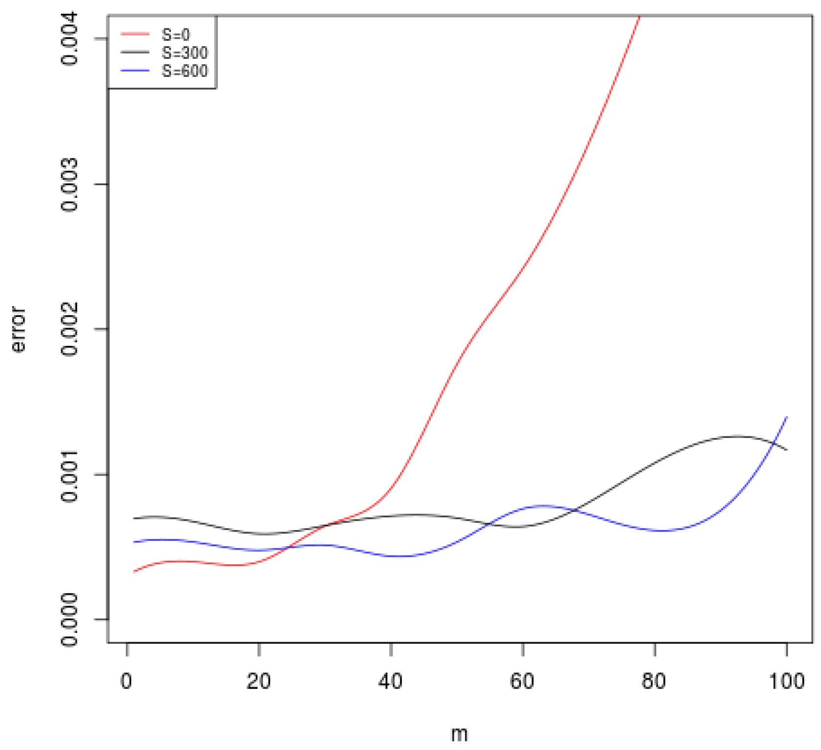
We apply the kernel K to the distributed algorithm (Equation (3)). In Figure 1, we plot the mean squared error of Equation (3) for $N=600$ and $S=0,300,600$ when the number of local machines m varies. Note that $S=0,$ and it is a standard distributed MEE algorithm without unlabeled data. When m becomes large, the red curve increases dramatically. However, when we add 300 or 600 unlabeled data, the error curves begin to increase very slowly. This coincides with our theory that using unlabeled data can enlarge the range of m in the distributed method.

This paper studied the convergence rate of the distribute gradient descent MEE algorithm in a semi-supervised setting. Our results demonstrated that using additional unlabeled data can improve the learning performance of the distributed MEE algorithm, especially in enlarging the range of m to guarantee the learning rate. As we know, there are many gaps between theory and empirical studies. We regard this paper as mainly a theoretical paper and expect that the theoretical analysis give some guidance to real applications.

References

- Principe, J.C. Renyi’s entropy and Kernel perspectives. In Information Theoretic Learning; Springer: New York, NY, USA, 2010. [Google Scholar]
- Erdogmus, D.; Principe, J.C. Comparison of entropy and mean square error criteria in adaptive system training using higher order statistics. In Proceedings of the International Conference on ICA and Signal Separation; Springer: Berlin, Germany, 2000; pp. 75–90. [Google Scholar]
- Erdogmus, D.; Hild, K.; Principe, J.C. Blind source separation using Renyi’s α-marginal entropies. Neurocomputing 2002, 49, 25–38. [Google Scholar] [CrossRef]
- Erdogmus, D.; Principe, J.C. Convergence properties and data efficiency of the minimum error entropy criterion in adaline training. IEEE Trans. Signal Process. 2003, 51, 1966–1978. [Google Scholar] [CrossRef]
- Gokcay, E.; Principe, J.C. Information theoretic clustering. IEEE Trans. Pattern Anal. Mach. Learn. 2002, 24, 158–171. [Google Scholar] [CrossRef]
- Silva, L.M.; Marques, J.; Alexandre, L.A. Neural network classification using Shannon’s entropy. In Proceedings of the European Symposium on Artificial Neural Networks; D-Side: Bruges, Belgium, 2005; pp. 217–222. [Google Scholar]
- Silva, L.M.; Marques, J.; Alexandre, L.A. The MEE principle in data classification: A perceptron-based analysis. Neural Comput. 2010, 22, 2698–2728. [Google Scholar] [CrossRef]
- Choe, Y. Information criterion for minimum cross-entropy model selection. arXiv, 2017; arXiv:1704.04315. [Google Scholar]
- Ying, Y.; Zhou, D.X. Online pairwise learning algorithms. Neural Comput. 2016, 28, 743–777. [Google Scholar] [CrossRef] [PubMed]
- Zhang, Y.; Duchi, J.C.; Wainwright, M.J. Divide and conquer kernel ridge regression: A dis tributed algorithm with minimax optimal rates. J. Mach. Learn. Res. 2013, 30, 592–617. [Google Scholar]
- Chapelle, O.; Zien, A. Semi-Supervised Learning (Adaptive Computation and Machine Learning); The MIT Press: Cambridge, MA, USA, 2006. [Google Scholar]
- Zhang, T. Learning bounds for kernel regression using effective data dimensionality. Neural Comput. 2005, 17, 2077–2098. [Google Scholar] [CrossRef] [PubMed]
- Caponnetto, A.; Vito, E.D. Optimal rates for the regularized least-squares algorithm. Found. Comput. Math. 2007, 7, 331–368. [Google Scholar] [CrossRef]
- Steinwart, I.; Hush, D.R.; Scovel, C. Optimal rates for regularized least squares regression. In Proceedings of the COLT 2009—the Conference on Learning Theory, Montreal, QC, Canada, 18–21 June 2009. [Google Scholar]
- Lin, S.B.; Guo, X.; Zhou, D.X. Distributed learning with regularized least squares. J. Mach. Learn. Res. 2017, 18, 3202–3232. [Google Scholar]
- Guo, Z.C.; Lin, S.B.; Zhou, D.X. Learning theory of distributed spectral algorithms. Inverse Prob. 2017, 33, 074009. [Google Scholar] [CrossRef]
- Guo, Z.C.; Shi, L.; Wu, Q. Learning theory of distributed regression with bias corrected regu-larization kernel network. J. Mach. Learn. Res. 2017, 18, 4237–4261. [Google Scholar]
- M<i>u</i>¨cke, N.; Blanchard, G. Parallelizing spectrally regularized kernel algorithms. J. Mach. Learn. Res. 2018, 19, 1069–1097. [Google Scholar]
- Lin, S.B.; Zhou, D.X. Distributed kernel-based gradient descent algorithms. Constr. Approx. 2018, 47, 249–276. [Google Scholar] [CrossRef]
- Yao, Y.; Rosasco, L.; Caponnetto, A. On early stopping in gradient descent learning. Constr. Approx. 2007, 26, 289–315. [Google Scholar] [CrossRef]
- Chang, X.; Lin, S.B.; Zhou, D.X. Distributed semi-supervised learning with kernel ridge re-gression. J. Mach. Learn. Res. 2017, 18, 1493–1514. [Google Scholar]
- Hu, T.; Wu, Q.; Zhou, D.X. Distributed kernel gradient descent algorithm for minimum error entropy principle. Unpublished work. 2018. [Google Scholar]
- Guo, X.; Hu, T.; Wu, Q. Distributed minimum error entropy algorithms. Unpublished work. 2018. [Google Scholar]
- Wang, B.; Hu, T. Distributed pairwise algorithms with gradient descent methods. Unpublished work. 2018. [Google Scholar]
Figure 1.
The mean square errors for the size of unlabeled data as the number of local machines m varies.