On f-Divergences: Integral Representations, Local Behavior, and Inequalities


Department of Electrical Engineering, Technion-Israel Institute of Technology, Haifa 3200003, Israel
Entropy 2018, 20(5), 383; https://0-doi-org.brum.beds.ac.uk/10.3390/e20050383
Submission received: 15 April 2018
/
Revised: 7 May 2018
/
Accepted: 15 May 2018
/
Published: 19 May 2018
(This article belongs to the Special Issue Entropy and Information Inequalities)
Abstract
:This paper is focused on f-divergences, consisting of three main contributions. The first one introduces integral representations of a general f-divergence by means of the relative information spectrum. The second part provides a new approach for the derivation of f-divergence inequalities, and it exemplifies their utility in the setup of Bayesian binary hypothesis testing. The last part of this paper further studies the local behavior of f-divergences.
1. Introduction
Probability theory, information theory, learning theory, statistical signal processing and other related disciplines, greatly benefit from non-negative measures of dissimilarity (a.k.a. divergence measures) between pairs of probability measures defined on the same measurable space (see, e.g., [1,2,3,4,5,6,7]). An axiomatic characterization of information measures, including divergence measures, was provided by Csiszár [8]. Many useful divergence measures belong to the set of f-divergences, independently introduced by Ali and Silvey [9], Csiszár [10,11,12,13], and Morimoto [14] in the early sixties. The family of f-divergences generalizes the relative entropy (a.k.a. the Kullback- Leibler divergence) while also satisfying the data processing inequality among other pleasing properties (see, e.g., [3] and references therein).
Integral representations of f-divergences serve to study properties of these information measures, and they are also used to establish relations among these divergences. An integral representation of f-divergences, expressed by means of the DeGroot statistical information, was provided in [3] with a simplified proof in [15]. The importance of this integral representation stems from the operational meaning of the DeGroot statistical information [16], which is strongly linked to Bayesian binary hypothesis testing. Some earlier specialized versions of this integral representation were introduced in [17,18,19,20,21], and a variation of it also appears in [22] Section 5.B. Implications of the integral representation of f-divergences, by means of the DeGroot statistical information, include an alternative proof of the data processing inequality, and a study of conditions for the sufficiency or -deficiency of observation channels [3,15].
Since many distance measures of interest fall under the paradigm of an f-divergence [23], bounds among f-divergences are very useful in many instances such as the analysis of rates of convergence and concentration of measure bounds, hypothesis testing, testing goodness of fit, minimax risk in estimation and modeling, strong data processing inequalities and contraction coefficients, etc. Earlier studies developed systematic approaches to obtain f-divergence inequalities while dealing with pairs of probability measures defined on arbitrary alphabets. A list of some notable existing f-divergence inequalities is provided, e.g., in [22] Section 1 and [23] Section 3. State-of-the-art techniques which serve to derive bounds among f-divergences include:
- (1)
- (2)
- Inequalities which rely on a characterization of the exact locus of the joint range of f-divergences [29];
- (3)
- (4)
- Sharp f-divergence inequalities by using numerical tools for maximizing or minimizing an f-divergence subject to a finite number of constraints on other f-divergences [33];
- (5)
- (6)
- (7)
- (8)
- (9)
- Bounds among f-divergences (or functions of f-divergences such as the Rényi divergence) via integral representations of these divergence measures [22] Section 8;
- (10)
- Inequalities which rely on variational representations of f-divergences (e.g., [54] Section 2).
Following earlier studies of the local behavior of f-divergences and their asymptotic properties (see related results by Csiszár and Shields [55] Theorem 4.1, Pardo and Vajda [56] Section 3, and Sason and Vérdu [22] Section 3.F), it is known that the local behavior of f-divergences scales, such as the chi-square divergence (up to a scaling factor which depends on f) provided that the first distribution approaches the reference measure in a certain strong sense. The study of the local behavior of f-divergences is an important aspect of their properties, and we further study it in this work.
This paper considers properties of f-divergences, while first introducing in Section 2 the basic definitions and notation needed, and in particular the various measures of dissimilarity between probability measures used throughout this paper. The presentation of our new results is then structured as follows:
Section 3 is focused on the derivation of new integral representations of f-divergences, expressed as a function of the relative information spectrum of the pair of probability measures, and the convex function f. The novelty of Section 3 is in the unified approach which leads to integral representations of f-divergences by means of the relative information spectrum, where the latter cumulative distribution function plays an important role in information theory and statistical decision theory (see, e.g., [7,54]). Particular integral representations of the type of results introduced in Section 3 have been recently derived by Sason and Verdú in a case-by-case basis for some f-divergences (see [22] Theorems 13 and 32), while lacking the approach which is developed in Section 3 for general f-divergences. In essence, an f-divergence is expressed in Section 3 as an inner product of a simple function of the relative information spectrum (depending only on the probability measures P and Q), and a non-negative weight function which only depends on f. This kind of representation, followed by a generalized result, serves to provide new integral representations of various useful f-divergences. This also enables in Section 3 to characterize the interplay between the DeGroot statistical information (or between another useful family of f-divergence, named the divergence with ) and the relative information spectrum.
Section 4 provides a new approach for the derivation of f-divergence inequalities, where an arbitrary f-divergence is lower bounded by means of the divergence [57] or the DeGroot statistical information [16]. The approach used in Section 4 yields several generalizations of the Bretagnole-Huber inequality [58], which provides a closed-form and simple upper bound on the total variation distance as a function of the relative entropy; the Bretagnole-Huber inequality has been proved to be useful, e.g., in the context of lower bounding the minimax risk in non-parametric estimation (see, e.g., [5] pp. 89–90, 94), and in the problem of density estimation (see, e.g., [6] Section 1.6). Although Vajda’s tight lower bound in [59] is slightly tighter everywhere than the Bretagnole-Huber inequality, our motivation for the generalization of the latter bound is justified later in this paper. The utility of the new inequalities is exemplified in the setup of Bayesian binary hypothesis testing.
Section 5 finally derives new results on the local behavior of f-divergences, i.e., the characterization of their scaling when the pair of probability measures are sufficiently close to each other. The starting point of our analysis in Section 5 relies on the analysis in [56] Section 3, regarding the asymptotic properties of f-divergences.
2. Preliminaries and Notation
We assume throughout that the probability measures P and Q are defined on a common measurable space , and denotes that P is absolutely continuous with respect to Q, namely there is no event such that .
Definition 1.
The relative information provided byaccording to, where, is given by
More generally, even if, let R be an arbitrary dominating probability measure such that(e.g.,); irrespectively of the choice of R, the relative information is defined to be
The following asymmetry property follows from (2):
Definition 2.
The relative information spectrum is the cumulative distribution function
The relative entropy is the expected valued of the relative information when it is distributed according to P:
Throughout this paper, denotes the set of convex functions with . Hence, the function is in ; if , then for all ; and if , then . We next provide a general definition for the family of f-divergences (see [3] p. 4398).
Definition 3
We rely in this paper on the following properties of f-divergences:
Proposition 1.
Let. The following conditions are equivalent:
- (1)
- (2)
- there exists a constantsuch that
Proposition 2.
Let, and letbe the conjugate function, given by
for. Then,; , and for every pair of probability measures,
By an analytic extension of in (12) at , let
Note that the convexity of implies that . In continuation to Definition 3, we get
with the convention in (16) that , We refer in this paper to the following f-divergences:
- (1)
- Relative entropy:with
- (2)
- (3)
- Some of the significance of the Hellinger divergence stems from the following facts:
- -
- The analytic extension of at yields
- -
- The chi-squared divergence [61] is the second order Hellinger divergence (see, e.g., [62] p. 48), i.e.,Note that, due to Proposition 1,where can be defined as
- -
- -
- -
- The Rényi divergence of order is a one-to-one transformation of the Hellinger divergence of the same order [11] (14):
- -
- The Alpha-divergence of order , as it is defined in [64] and ([65] (4)), is a generalized relative entropy which (up to a scaling factor) is equal to the Hellinger divergence of the same order . More explicitly,where denotes the Alpha-divergence of order . Note, however, that the Beta and Gamma-divergences in [65], as well as the generalized divergences in [66,67], are not f-divergences in general.
- (4)
- Specifically, for , letand the total variation distance is expressed as an f-divergence:
- (5)
- Note that
- (6)
- The special case of (41) with gives the Jensen-Shannon divergence (a.k.a. capacitory discrimination):
- (7)
- (8)
- The following relation to the total variation distance holds:and the DeGroot statistical information and the divergence are related as follows [22] (384):
3. New Integral Representations of -Divergences
The main result in this section provides new integral representations of f-divergences as a function of the relative information spectrum (see Definition 2). The reader is referred to other integral representations (see [15] Section 2, [4] Section 5, [22] Section 5.B, and references therein), expressing a general f-divergence by means of the DeGroot statistical information or the divergence.
Lemma 1.
Letbe a strictly convex function at 1. Letbe defined as
wheredenotes the right-hand derivative of f at 1 (due to the convexity of f on, it exists and it is finite). Then, the function g is non-negative, it is strictly monotonically decreasing on, and it is strictly monotonically increasing onwith.
Proof.
For any function , let be given by
and let be the conjugate function, as given in (12). The function g in (54) can be expressed in the form
as it is next verified. For , we get from (12) and (55),
and the substitution for yields (56) in view of (54).
By assumption, is strictly convex at 1, and therefore these properties are inherited to . Since also , it follows from [3] Theorem 3 that both and are non-negative on , and they are also strictly monotonically decreasing on . Hence, from (12), it follows that the function is strictly monotonically increasing on . Finally, the claimed properties of the function g follow from (56), and in view of the fact that the function is non-negative with , strictly monotonically decreasing on and strictly monotonically increasing on . ☐
Lemma 2.
Letbe a strictly convex function at 1, and letbe as in (54). Let
and let and be the two inverse functions of g. Then,
Proof.
In view of Lemma 1, it follows that is strictly monotonically increasing and is strictly monotonically decreasing with .
Let , and let . Then, we have
where (61) relies on Proposition 1; (62) relies on Proposition 2; (64) follows from (3); (65) follows from (56); (66) holds by the definition of the random variable V; (67) holds since, in view of Lemma 1, , and for any non-negative random variable Z; (68) holds in view of the monotonicity properties of g in Lemma 1, the definition of a and b in (58) and (59), and by expressing the event as a union of two disjoint events; (69) holds again by the monotonicity properties of g in Lemma 1, and by the definition of its two inverse functions and as above; in (67)–(69) we are free to substitute > by ≥, and < by ≤; finally, (70) holds by the definition of the relative information spectrum in (4). ☐
Remark 1.
The functionin (54) is invariant to the mapping , for , with an arbitrary . This invariance of g (and, hence, also the invariance of its inverse functions and ) is well expected in view of Proposition 1 and Lemma 2.
Example 1.
Lemma 3.
Proof.
Remark 2.
Unlike Example 1, in general, the inverse functionsandin Lemma 2 are not expressible in closed form, motivating our next integral representation in Theorem 1.
The following theorem provides our main result in this section.
Theorem 1.
The following integral representations of an f-divergence, by means of the relative information spectrum, hold:
- (1)
- Let
- -
- be differentiable on;
- -
- be the non-negative weight function given, for, by
- -
- the functionbe given by
Then, - (2)
- More generally, for an arbitrary, letbe a modified real-valued function defined asThen,
Proof.
We start by proving the special integral representation in (81), and then extend our proof to the general representation in (83).
- (1)
- We first assume an additional requirement that f is strictly convex at 1. In view of Lemma 2,Since by assumption is differentiable on and strictly convex at 1, the function g in (54) is differentiable on . In view of (84) and (85), substituting in (60) for implies thatwhere is given byfor , where (88) follows from (54). Due to the monotonicity properties of g in Lemma 1, (87) implies that for , and for . Hence, the weight function in (79) satisfiesWe now extend the result in (81) when is differentiable on , but not necessarily strictly convex at 1. To that end, let be defined asThis implies that is differentiable on , and it is also strictly convex at 1. In view of the proof of (81) when f is strict convexity of f at 1, the application of this result to the function s in (90) yieldsIn view of (6), (22), (23), (25) and (90),from (79), (89), (90) and the convexity and differentiability of , it follows that the weight function satisfiesfor . Furthermore, by applying the result in (81) to the chi-squared divergence in (25) whose corresponding function for is strictly convex at 1, we obtain
- (2)
Remark 3.
Remark 4.
Remark 5.
An equivalent way to writein (80) is
where . Hence, the function is monotonically increasing in , and it is monotonically decreasing in ; note that this function is in general discontinuous at 1 unless . If , then
Note that if, thenis zero everywhere, which is consistent with the fact that.
Remark 6.
In the proof of Theorem 1-(1), the relaxation of the condition of strict convexity at 1 for a differentiable function is crucial, e.g., for the divergence with . To clarify this claim, note that in view of (32), the function is differentiable if , and with ; however, if , so in not strictly convex at 1 unless .
Remark 7.
Theorem 1-(1) with enables, in some cases, to simplify integral representations of f-divergences. This is next exemplified in the proof of Theorem 2.
Theorem 1 yields integral representations for various f-divergences and related measures; some of these representations were previously derived by Sason and Verdú in [22] in a case by case basis, without the unified approach of Theorem 1. We next provide such integral representations. Note that, for some f-divergences, the function is not differentiable on ; hence, Theorem 1 is not necessarily directly applicable.
Theorem 2.
The following integral representations hold as a function of the relative information spectrum:
- (1)
- Relative entropy [22] (219):
- (2)
- Hellinger divergence of order [22] (434) and (437):
- (3)
- Rényi divergence [22] (426) and (427): For ,
- (4)
- divergence: For
- (5)
- DeGroot statistical information:
- (6)
- Triangular discrimination:
- (7)
- Lin’s measure: For ,where denotes the binary entropy function. Specifically, the Jensen-Shannon divergence admits the integral representation:
- (8)
- Jeffrey’s divergence:
- (9)
- divergence: For ,
Proof.
See Appendix A. ☐
An application of (112) yields the following interplay between the divergence and the relative information spectrum.
Theorem 3.
Let , and let the random variable have no probability masses. Denote
Then,
- is a continuously differentiable function of γ on , and ;
- the sets and determine, respectively, the relative information spectrum on and ;
- for ,
Proof.
We start by proving the first item. By our assumption, is continuous on . Hence, it follows from (112) that is continuously differentiable in ; furthermore, (45) implies that is monotonically decreasing in , which yields .
We next prove the second and third items together. Let and . From (112), for ,
which yields (115). Due to the continuity of , it follows that the set determines the relative information spectrum on .
To prove (116), we have
where (120) holds by switching P and Q in (46); (121) holds since ; (122) holds by switching P and Q in (115) (correspondingly, also and are switched); (123) holds since ; (124) holds by the assumption that has no probability masses, which implies that the sign < can be replaced with ≤ at the term in the right side of (123). Finally, (116) readily follows from (120)–(124), which implies that the set determines on .
A similar application of (107) yields an interplay between DeGroot statistical information and the relative information spectrum.
Theorem 4.
Let , and let the random variable have no probability masses. Denote
Then,
- is a continuously differentiable function of ω on ,and is, respectively, non-negative or non-positive on and ;
- the sets and determine, respectively, the relative information spectrum on and ;
- forforand
Remark 8.
By relaxing the condition in Theorems 3 and 4 where has no probability masses with , it follows from the proof of Theorem 3 that each one of the sets
determines at every point on where this relative information spectrum is continuous. Note that, as a cumulative distribution function, is discontinuous at a countable number of points. Consequently, under the condition that is differentiable on , the integral representations of in Theorem 1 are not affected by the countable number of discontinuities for .
In view of Theorems 1, 3 and 4 and Remark 8, we get the following result.
Corollary 1.
Remark 9.
Corollary 1 is supported by the integral representation of in [3] Theorem 11, expressed as a function of the set of values in , and its analogous representation in [22] Proposition 3 as a function of the set of values in . More explicitly, [3] Theorem 11 states that if , then
where is a certain σ-finite measure defined on the Borel subsets of ; it is also shown in [3] (80) that if is twice differentiable on , then
4. New -Divergence Inequalities
Various approaches for the derivation of f-divergence inequalities were studied in the literature (see Section 1 for references). This section suggests a new approach, leading to a lower bound on an arbitrary f-divergence by means of the divergence of an arbitrary order (see (45)) or the DeGroot statistical information (see (50)). This approach leads to generalizations of the Bretagnole-Huber inequality [58], whose generalizations are later motivated in this section. The utility of the f-divergence inequalities in this section is exemplified in the setup of Bayesian binary hypothesis testing.
In the following, we provide the first main result in this section for the derivation of new f-divergence inequalities by means of the divergence. Generalizing the total variation distance, the divergence in (45)–(47) is an f-divergence whose utility in information theory has been exemplified in [17] Chapter 3, [54],[57] p. 2314 and [69]; the properties of this measure were studied in [22] Section 7 and [54] Section 2.B.
Theorem 5.
Let , and let be the conjugate convex function as defined in (12). Let P and Q be probability measures. Then, for all ,
Proof.
Let and be the densities of P and Q with respect to a dominating measure . Then, for an arbitrary ,
where (139) follows from the convexity of and by invoking Jensen’s inequality.
An application of Theorem 5 gives the following lower bounds on the Hellinger and Rényi divergences with arbitrary positive orders, expressed as a function of the divergence with an arbitrary order .
Corollary 2.
For all and ,
and
Proof.
Corollary 3.
For , the following upper bounds on divergence hold as a function of the relative entropy and divergence:
Remark 10.
From [4] (58),
is a tight lower bound on the chi-squared divergence as a function of the total variation distance. In view of (49), we compare (151) with the specialized version of (149) when . The latter bound is expected to be looser than the tight bound in (151), as a result of the use of Jensen’s inequality in the proof of Theorem 5; however, it is interesting to examine how much we loose in the tightness of this specialized bound with . From (49), the substitution of in (149) gives
and, it can be easily verified that
Inequality (153) forms a counterpart to Pinsker’s inequality:
proved by Csiszár [12] and Kullback [70], with Kemperman [71] independently a bit later. As upper bounds on the total variation distance, (154) outperforms (153) if nats, and (153) outperforms (154) for larger values of .
Remark 12.
In [59] (8), Vajda introduced a lower bound on the relative entropy as a function of the total variation distance:
The lower bound in the right side of (155) is asymptotically tight in the sense that it tends to ∞ if , and the difference between and this lower bound is everywhere upper bounded by (see [59] (9)). The Bretagnole-Huber inequality in (153), on the other hand, is equivalent to
Although it can be verified numerically that the lower bound on the relative entropy in (155) is everywhere slightly tighter than the lower bound in (156) (for ), both lower bounds on are of the same asymptotic tightness in a sense that they both tend to ∞ as and their ratio tends to 1. Apart of their asymptotic tightness, the Bretagnole-Huber inequality in (156) is appealing since it provides a closed-form simple upper bound on as a function of (see (153)), whereas such a closed-form simple upper bound cannot be obtained from (155). In fact, by the substitution and the exponentiation of both sides of (155), we get the inequality whose solution is expressed by the Lambert W function [72]; it can be verified that (155) is equivalent to the following upper bound on the total variation distance as a function of the relative entropy:
where W in the right side of (157) denotes the principal real branch of the Lambert W function. The difference between the upper bounds in (153) and (157) can be verified to be marginal if is large (e.g., if nats, then the upper bounds on are respectively equal to 1.982 and 1.973), though the former upper bound in (153) is clearly more simple and amenable to analysis.
The Bretagnole-Huber inequality in (153) is proved to be useful in the context of lower bounding the minimax risk (see, e.g., [5] pp. 89–90, 94), and the problem of density estimation (see, e.g., [6] Section 1.6). The utility of this inequality motivates its generalization in this section (see Corollaries 2 and 3, and also see later Theorem 7 followed by Example 2).
In [22] Section 7.C, Sason and Verdú generalized Pinsker’s inequality by providing an upper bound on the divergence, for , as a function of the relative entropy. In view of (49) and the optimality of the constant in Pinsker’s inequality (154), it follows that the minimum achievable is quadratic in for small values of . It has been proved in [22] Section 7.C that this situation ceases to be the case for , in which case it is possible to upper bound as a constant times where this constant tends to infinity as we let . We next cite the result in [22] Theorem 30, extending (154) by means of the divergence for , and compare it numerically to the bound in (150).
Theorem 6.
As an immediate consequence of (159), it follows that
which forms a straight-line bound on the divergence as a function of the relative entropy for . Similarly to the comparison of the Bretagnole-Huber inequality (153) and Pinsker’s inequality (154), we exemplify numerically that the extension of Pinsker’s inequality to the divergence in (162) forms a counterpart to the generalized version of the Bretagnole-Huber inequality in (150).
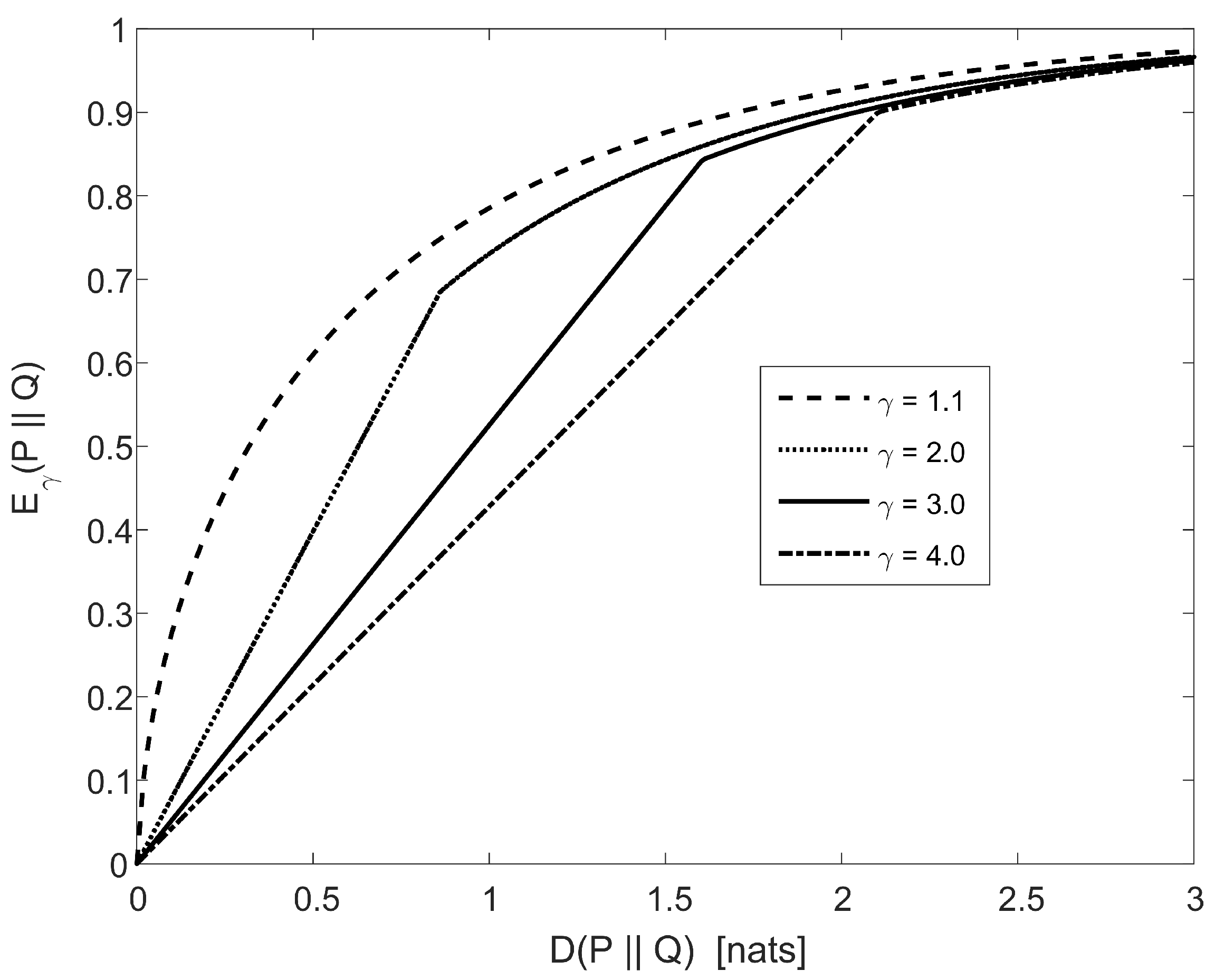
Figure 1 plots an upper bound on the divergence, for , as a function of the relative entropy (or, alternatively, a lower bound on the relative entropy as a function of the divergence). The upper bound on for , as a function of , is composed of the following two components:
It is supported by Figure 1 that is positive and monotonically increasing, and ; e.g., it can be verified that , , , and (see Figure 1).
Bayesian Binary Hypothesis Testing
The DeGroot statistical information [16] has the following meaning: consider two hypotheses and , and let and with . Let P and Q be probability measures, and consider an observation Y where , and . Suppose that one wishes to decide which hypothesis is more likely given the observation Y. The operational meaning of the DeGroot statistical information, denoted by , is that this measure is equal to the minimal difference between the a-priori error probability (without side information) and a posteriori error probability (given the observation Y). This measure was later identified as an f-divergence by Liese and Vajda [3] (see (50) here).
Theorem 7.
The DeGroot statistical information satisfies the following upper bound as a function of the chi-squared divergence:
and the following bounds as a function of the relative entropy:
- (1)
- (2)
Proof.
Remark 13.
Remark 15.
The upper bounds on in (163) and (165) are asymptotically tight when we let and tend to infinity. To verify this, first note that (see [23] Theorem 5)
which implies that also and tend to infinity. In this case, it can be readily verified that the bounds in (163) and (165) are specialized to ; this upper bound, which is equal to the a-priori error probability, is also equal to the DeGroot statistical information since the a-posterior error probability tends to zero in the considered extreme case where P and Q are sufficiently far from each other, so that and are easily distinguishable in high probability when the observation Y is available.
Remark 16.
Due to the one-to-one correspondence between the divergence and DeGroot statistical information in (53), which shows that the two measures are related by a multiplicative scaling factor, the numerical results shown in Figure 1 also apply to the bounds in (164) and (165); i.e., for , the first bound in (164) is tighter than the second bound in (165) for small values of the relative entropy, whereas (165) becomes tighter than (164) for larger values of the relative entropy.
Corollary 4.
- (1)
- for ,
- (2)
- for ,
We end this section by exemplifying the utility of the bounds in Theorem 7.
Example 2.
Let and with , and assume that the observation Y given that the hypothesis is or is Poisson distributed with the positive parameter μ or λ, respectively:
where
Without any loss of generality, let . The bounds on the DeGroot statistical information in Theorem 7 can be expressed in a closed form by relying on the following identities:
To simplify the right side of (174), let , and define
where for , denotes the largest integer that is smaller than or equal to x. It can be verified that
To exemplify the utility of the bounds in Theorem 7, suppose that μ and λ are close, and we wish to obtain a guarantee on how small is. For example, let , , and . The upper bounds on in (163)–(165) are, respectively, equal to , and ; we therefore get an informative guarantee by easily calculable bounds. The exact value of is, on the other hand, hard to compute since (see (175)), and the calculation of the right side of (178) appears to be sensitive to the selected parameters in this setting.
5. Local Behavior of f-Divergences
This section studies the local behavior of f-divergences; the starting point relies on [56] Section 3 which studies the asymptotic properties of f-divergences. The reader is also referred to a related study in [22] Section 4.F.
Lemma 4.
Let
- be a sequence of probability measures on a measurable space ;
- the sequence converge to a probability measure Q in the sense thatwhere for all sufficiently large n;
- have continuous second derivatives at 1 and .
Then
Proof.
The result in (180) follows from [56] Theorem 3, even without the additional restriction in [56] Section 3 which would require that the second derivatives of f and g are locally Lipschitz at a neighborhood of 1. More explicitly, in view of the analysis in [56] p. 1863, we get by relaxing the latter restriction that (cf. [56] (31))
where as we let , and also
Remark 17.
Since f and g in Lemma 4 are assumed to have continuous second derivatives at 1, the left and right derivatives of the weight function in (79) at 1 satisfy, in view of Remark 3,
Lemma 5.
Proof.
Let and be the densities of P and Q with respect to an arbitrary probability measure such that . Then,
☐
Remark 18.
The result in Lemma 5, for the chi-squared divergence, is generalized to the identity
Remark 19.
The result in Lemma 5 can be generalized as follows: let be probability measures, and . Let for an arbitrary probability measure μ, and , , and be the corresponding densities with respect to μ. Calculation shows that
with
We next state the main result in this section.
Theorem 8.
Let
- P and Q be probability measures defined on a measurable space , , and suppose that
- , and be continuous at 1.
Then,
Proof.
Let be a sequence in , which tends to zero. Define the sequence of probability measures
Consequently, (183) implies that
where in (197) is an arbitrary sequence which tends to zero. Hence, it follows from (197) and (200) that
and, by combining (186) and (201), we get
We next prove the result for the limit in the right side of (195). Let be the conjugate function of f, which is given in (12). By the assumption that f has a second continuous derivative, so is and it is easy to verify that the second derivatives of f and coincide at 1. Hence, from (13) and (202),
☐
Remark 20.
Although an f-divergence is in general not symmetric, in the sense that the equality does not necessarily hold for all pairs of probability measures , the reason for the equality in (195) stems from the fact that the second derivatives of f and coincide at 1 when f is twice differentiable.
Remark 21.
The following result refers to the local behavior of Rényi divergences of an arbitrary non-negative order.
Corollary 5.
Acknowledgments
The author is grateful to Sergio Verdú and the two anonymous reviewers, whose suggestions improved the presentation in this paper.
Conflicts of Interest
The author declares no conflict of interest.
Appendix A. Proof of Theorem 2
We prove in the following the integral representations of f-divergences and related measures in Theorem 2.
- (1)
- (2)
- Hellinger divergence: In view of (22), for , the weight function in (79) which corresponds to in (23) can be verified to be equal tofor . In order to simplify the integral representation of the Hellinger divergence , we apply Theorem 1-(1). From (A3), setting in (82) implies that is given byfor . Hence, substituting (80) and (A4) into (83) yieldsThis proves (99). We next consider the following special cases:
- (3)
- (4)
- (5)
- DeGroot statistical information: In view of (50)–(51), since the function is not differentiable at the point for , Theorem 1 cannot be applied directly to get an integral representation of the DeGroot statistical information. To that end, for , consider the family of convex functions given by (see [3] (55))for . These differentiable functions also satisfywhich holds due to the identitiesThe application of Theorem 1-(1) to the set of functions withyieldsfor , andwith as defined in (80), and . From (A15) and (A18), it follows thatfor . In view of (50), (51), (80), (A14), (A19) and (A20), and the monotone convergence theorem,for . We next simplify (A23) as follows:
- -
- if , then and (A23) yields
- -
- (6)
- (7)
- (8)
- (9)
- divergence: Let , and let satisfy ; hence, . From (53), we getThe second line in the right side of (107) yields
Remark A1.
References
- Basseville, M. Divergence measures for statistical data processing—An annotated bibliography. Signal Process. 2013, 93, 621–633. [Google Scholar] [CrossRef]
- Liese, F.; Vajda, I. Convex Statistical Distances. In Teubner-Texte Zur Mathematik; Springer: Leipzig, Germany, 1987; Volume 95. [Google Scholar]
- Liese, F.; Vajda, I. On divergences and informations in statistics and information theory. IEEE Trans. Inf. Theory 2006, 52, 4394–4412. [Google Scholar] [CrossRef]
- Reid, M.D.; Williamson, R.C. Information, divergence and risk for binary experiments. J. Mach. Learn. Res. 2011, 12, 731–817. [Google Scholar]
- Tsybakov, A.B. Introduction to Nonparametric Estimation; Springer: New York, NY, USA, 2009. [Google Scholar]
- Vapnik, V.N. Statistical Learning Theory; John Wiley & Sons: Hoboken, NJ, USA, 1998. [Google Scholar]
- Verdú, S. Information Theory. Unpublished work. 2018. [Google Scholar]
- Csiszár, I. Axiomatic characterization of information measures. Entropy 2008, 10, 261–273. [Google Scholar] [CrossRef]
- Ali, S.M.; Silvey, S.D. A general class of coefficients of divergence of one distribution from another. J. R. Stat. Soc. Ser. B 1966, 28, 131–142. [Google Scholar]
- Csiszár, I. Eine Informationstheoretische Ungleichung und ihre Anwendung auf den Bewis der Ergodizität von Markhoffschen Ketten. Magyer Tud. Akad. Mat. Kutato Int. Koezl. 1963, 8, 85–108. [Google Scholar]
- Csiszár, I. A note on Jensen’s inequality. Stud. Sci. Math. Hung. 1966, 1, 185–188. [Google Scholar]
- Csiszár, I. Information-type measures of difference of probability distributions and indirect observations. Stud. Sci. Math. Hung. 1967, 2, 299–318. [Google Scholar]
- Csiszár, I. On topological properties of f-divergences. Stud. Sci. Math. Hung. 1967, 2, 329–339. [Google Scholar]
- Morimoto, T. Markov processes and the H-theorem. J. Phys. Soc. Jpn. 1963, 18, 328–331. [Google Scholar] [CrossRef]
- Liese, F. φ-divergences, sufficiency, Bayes sufficiency, and deficiency. Kybernetika 2012, 48, 690–713. [Google Scholar]
- DeGroot, M.H. Uncertainty, information and sequential experiments. Ann. Math. Stat. 1962, 33, 404–419. [Google Scholar] [CrossRef]
- Cohen, J.E.; Kemperman, J.H.B.; Zbăganu, G. Comparisons of Stochastic Matrices with Applications in Information Theory, Statistics, Economics and Population; Springer: Berlin, Germany, 1998. [Google Scholar]
- Feldman, D.; Österreicher, F. A note on f-divergences. Stud. Sci. Math. Hung. 1989, 24, 191–200. [Google Scholar]
- Guttenbrunner, C. On applications of the representation of f-divergences as averaged minimal Bayesian risk. In Proceedings of the Transactions of the 11th Prague Conferences on Information Theory, Statistical Decision Functions, and Random Processes, Prague, Czechoslovakia, 26–31 August 1992; pp. 449–456. [Google Scholar]
- Österreicher, F.; Vajda, I. Statistical information and discrimination. IEEE Trans. Inf. Theory 1993, 39, 1036–1039. [Google Scholar] [CrossRef]
- Torgersen, E. Comparison of Statistical Experiments; Cambridge University Press: Cambridge, UK, 1991. [Google Scholar]
- Sason, I.; Verdú, S. f-divergence inequalities. IEEE Trans. Inf. Theory 2016, 62, 5973–6006. [Google Scholar] [CrossRef]
- Gibbs, A.L.; Su, F.E. On choosing and bounding probability metrics. Int. Stat. Rev. 2002, 70, 419–435. [Google Scholar] [CrossRef]
- Anwar, M.; Hussain, S.; Pecaric, J. Some inequalities for Csiszár-divergence measures. Int. J. Math. Anal. 2009, 3, 1295–1304. [Google Scholar]
- Simic, S. On logarithmic convexity for differences of power means. J. Inequal. Appl. 2007, 2007, 37359. [Google Scholar] [CrossRef]
- Simic, S. On a new moments inequality. Stat. Probab. Lett. 2008, 78, 2671–2678. [Google Scholar] [CrossRef]
- Simic, S. On certain new inequalities in information theory. Acta Math. Hung. 2009, 124, 353–361. [Google Scholar] [CrossRef]
- Simic, S. Moment Inequalities of the Second and Third Orders. Preprint. Available online: http://arxiv.org/abs/1509.0851 (accessed on 13 May 2016).
- Harremoës, P.; Vajda, I. On pairs of f-divergences and their joint range. IEEE Trans. Inf. Theory 2011, 57, 3230–3235. [Google Scholar] [CrossRef]
- Sason, I.; Verdú, S. f-divergence inequalities via functional domination. In Proceedings of the 2016 IEEE International Conference on the Science of Electrical Engineering, Eilat, Israel, 16–18 November 2016; pp. 1–5. [Google Scholar]
- Taneja, I.J. Refinement inequalities among symmetric divergence measures. Aust. J. Math. Anal. Appl. 2005, 2, 1–23. [Google Scholar]
- Taneja, I.J. Seven means, generalized triangular discrimination, and generating divergence measures. Information 2013, 4, 198–239. [Google Scholar] [CrossRef]
- Guntuboyina, A.; Saha, S.; Schiebinger, G. Sharp inequalities for f-divergences. IEEE Trans. Inf. Theory 2014, 60, 104–121. [Google Scholar] [CrossRef]
- Endres, D.M.; Schindelin, J.E. A new metric for probability distributions. IEEE Trans. Inf. Theory 2003, 49, 1858–1860. [Google Scholar] [CrossRef] [Green Version]
- Kafka, P.; Östreicher, F.; Vincze, I. On powers of f-divergences defining a distance. Stud. Sci. Math. Hung. 1991, 26, 415–422. [Google Scholar]
- Lu, G.; Li, B. A class of new metrics based on triangular discrimination. Information 2015, 6, 361–374. [Google Scholar] [CrossRef]
- Vajda, I. On metric divergences of probability measures. Kybernetika 2009, 45, 885–900. [Google Scholar]
- Gilardoni, G.L. On Pinsker’s and Vajda’s type inequalities for Csiszár’s f-divergences. IEEE Trans. Inf. Theory 2010, 56, 5377–5386. [Google Scholar] [CrossRef]
- Topsøe, F. Some inequalities for information divergence and related measures of discrimination. IEEE Trans. Inf. Theory 2000, 46, 1602–1609. [Google Scholar] [CrossRef]
- Sason, I.; Verdú, S. Upper bounds on the relative entropy and Rényi divergence as a function of total variation distance for finite alphabets. In Proceedings of the 2015 IEEE Information Theory Workshop, Jeju Island, Korea, 11–15 October 2015; pp. 214–218. [Google Scholar]
- Dragomir, S.S. Upper and lower bounds for Csiszár f-divergence in terms of the Kullback-Leibler divergence and applications. In Inequalities for Csiszár f-Divergence in Information Theory, RGMIA Monographs; Victoria University: Footscray, VIC, Australia, 2000. [Google Scholar]
- Dragomir, S.S. Upper and lower bounds for Csiszár f-divergence in terms of Hellinger discrimination and applications. In Inequalities for Csiszár f-Divergence in Information Theory, RGMIA Monographs; Victoria University: Footscray, VIC, Australia, 2000. [Google Scholar]
- Dragomir, S.S. An upper bound for the Csiszár f-divergence in terms of the variational distance and applications. In Inequalities for Csiszár f-Divergence in Information Theory, RGMIA Monographs; Victoria University: Footscray, VIC, Australia, 2000. [Google Scholar]
- Dragomir, S.S.; Gluščević, V. Some inequalities for the Kullback-Leibler and χ2-distances in information theory and applications. Tamsui Oxf. J. Math. Sci. 2001, 17, 97–111. [Google Scholar]
- Dragomir, S.S. Bounds for the normalized Jensen functional. Bull. Aust. Math. Soc. 2006, 74, 471–478. [Google Scholar] [CrossRef]
- Kumar, P.; Chhina, S. A symmetric information divergence measure of the Csiszár’s f-divergence class and its bounds. Comp. Math. Appl. 2005, 49, 575–588. [Google Scholar] [CrossRef]
- Taneja, I.J. Bounds on non-symmetric divergence measures in terms of symmetric divergence measures. J. Comb. Inf. Syst. Sci. 2005, 29, 115–134. [Google Scholar]
- Binette, O. A note on reverse Pinsker inequalities. Preprint. Available online: http://arxiv.org/abs/1805.05135 (accessed on 14 May 2018).
- Gilardoni, G.L. On the minimum f-divergence for given total variation. C. R. Math. 2006, 343, 763–766. [Google Scholar] [CrossRef]
- Gilardoni, G.L. Corrigendum to the note on the minimum f-divergence for given total variation. C. R. Math. 2010, 348, 299. [Google Scholar] [CrossRef]
- Gushchin, A.A. The minimum increment of f-divergences given total variation distances. Math. Methods Stat. 2016, 25, 304–312. [Google Scholar] [CrossRef]
- Sason, I. Tight bounds on symmetric divergence measures and a refined bound for lossless source coding. IEEE Trans. Inf. Theory 2015, 61, 701–707. [Google Scholar] [CrossRef]
- Sason, I. On the Rényi divergence, joint range of relative entropies, and a channel coding theorem. IEEE Trans. Inf. Theory 2016, 62, 23–34. [Google Scholar] [CrossRef]
- Liu, J.; Cuff, P.; Verdú, S. Eγ-resolvability. IEEE Trans. Inf. Theory 2017, 63, 2629–2658. [Google Scholar]
- Csiszár, I.; Shields, P.C. Information Theory and Statistics: A Tutorial. Found. Trends Commun. Inf. Theory 2004, 1, 417–528. [Google Scholar] [CrossRef]
- Pardo, M.C.; Vajda, I. On asymptotic properties of information-theoretic divergences. IEEE Trans. Inf. Theory 2003, 49, 1860–1868. [Google Scholar] [CrossRef]
- Polyanskiy, Y.; Poor, H.V.; Verdú, S. Channel coding rate in the finite blocklength regime. IEEE Trans. Inf. Theory 2010, 56, 2307–2359. [Google Scholar] [CrossRef]
- Bretagnolle, J.; Huber, C. Estimation des densités: Risque minimax. Probab. Theory Relat. Fields 1979, 47, 119–137. [Google Scholar]
- Vajda, I. Note on discrimination information and variation. IEEE Trans. Inf. Theory 1970, 16, 771–773. [Google Scholar] [CrossRef]
- Jeffreys, H. An invariant form for the prior probability in estimation problems. Proc. R. Soc. Lond. Ser. A Math. Phys. Sci. 1946, 186, 453–461. [Google Scholar] [CrossRef]
- Pearson, K. On the criterion that a given system of deviations from the probable in the case of a correlated system of variables is such that it can be reasonably supposed to have arisen from random sampling. Lond. Edinb. Dublin Philos. Mag. J. Sci. 1900, 50, 157–175. [Google Scholar] [CrossRef]
- Le Cam, L. Asymptotic Methods in Statistical Decision Theory; Springer: New York, NY, USA, 1986. [Google Scholar]
- Kailath, T. The divergence and Bhattacharyya distance measures in signal selection. IEEE Trans. Commun. Technol. 1967, 15, 52–60. [Google Scholar] [CrossRef]
- Amari, S.I.; Nagaoka, H. Methods of Information Geometry; Oxford University Press: New York, NY, USA, 2000. [Google Scholar]
- Cichocki, A.; Amari, S.I. Families of Alpha- Beta- and Gamma-divergences: Flexible and robust measures of similarities. Entropy 2010, 12, 1532–1568. [Google Scholar] [CrossRef]
- Cichocki, A.; Cruces, S.; Amari, S.I. Generalized Alpha-Beta divergences and their application to robust nonnegative matrix factorization. Entropy 2011, 13, 134–170. [Google Scholar] [CrossRef]
- Cichocki, A.; Cruces, S.; Amari, S.I. Log-determinant divergences revisited: Alpha-Beta and Gamma log-det divergences. Entropy 2015, 17, 2988–3034. [Google Scholar] [CrossRef]
- Lin, J. Divergence measures based on the Shannon entropy. IEEE Trans. Inf. Theory 1991, 37, 145–151. [Google Scholar] [CrossRef]
- Polyanskiy, Y.; Wu, Y. Dissipation of information in channels with input constraints. IEEE Trans. Inf. Theory 2016, 62, 35–55. [Google Scholar] [CrossRef]
- Kullback, S. A lower bound for discrimination information in terms of variation. IEEE Trans. Inf. Theory 1967, 13, 126–127. [Google Scholar] [CrossRef]
- Kemperman, J.H.B. On the optimal rate of transmitting information. Ann. Math. Stat. 1969, 40, 2156–2177. [Google Scholar] [CrossRef]
- Corless, R.M.; Gonnet, G.H.; Hare, D.E.; Jeffrey, D.J.; Knuth, D.E. On the Lambert W function. Adv. Comput. Math. 1996, 5, 329–359. [Google Scholar] [CrossRef]
- Van Erven, T.; Harremoës, P. Rényi divergence and Kullback-Leibler divergence. IEEE Trans. Inf. Theory 2014, 60, 3797–3820. [Google Scholar] [CrossRef]

© 2018 by the author. Licensee MDPI, Basel, Switzerland. This article is an open access article distributed under the terms and conditions of the Creative Commons Attribution (CC BY) license (http://creativecommons.org/licenses/by/4.0/).
Share and Cite
MDPI and ACS Style
Sason, I. On f-Divergences: Integral Representations, Local Behavior, and Inequalities. Entropy 2018, 20, 383. https://0-doi-org.brum.beds.ac.uk/10.3390/e20050383
AMA Style
Sason I. On f-Divergences: Integral Representations, Local Behavior, and Inequalities. Entropy. 2018; 20(5):383. https://0-doi-org.brum.beds.ac.uk/10.3390/e20050383
Chicago/Turabian StyleSason, Igal. 2018. "On f-Divergences: Integral Representations, Local Behavior, and Inequalities" Entropy 20, no. 5: 383. https://0-doi-org.brum.beds.ac.uk/10.3390/e20050383
Note that from the first issue of 2016, this journal uses article numbers instead of page numbers. See further details here.