This section deals with the theoretical and graphical behavior of different physical quantities that are obtained in the present flow problem. The computational software Mathematica has been utilized to investigate the novelties of all the physical parameters.
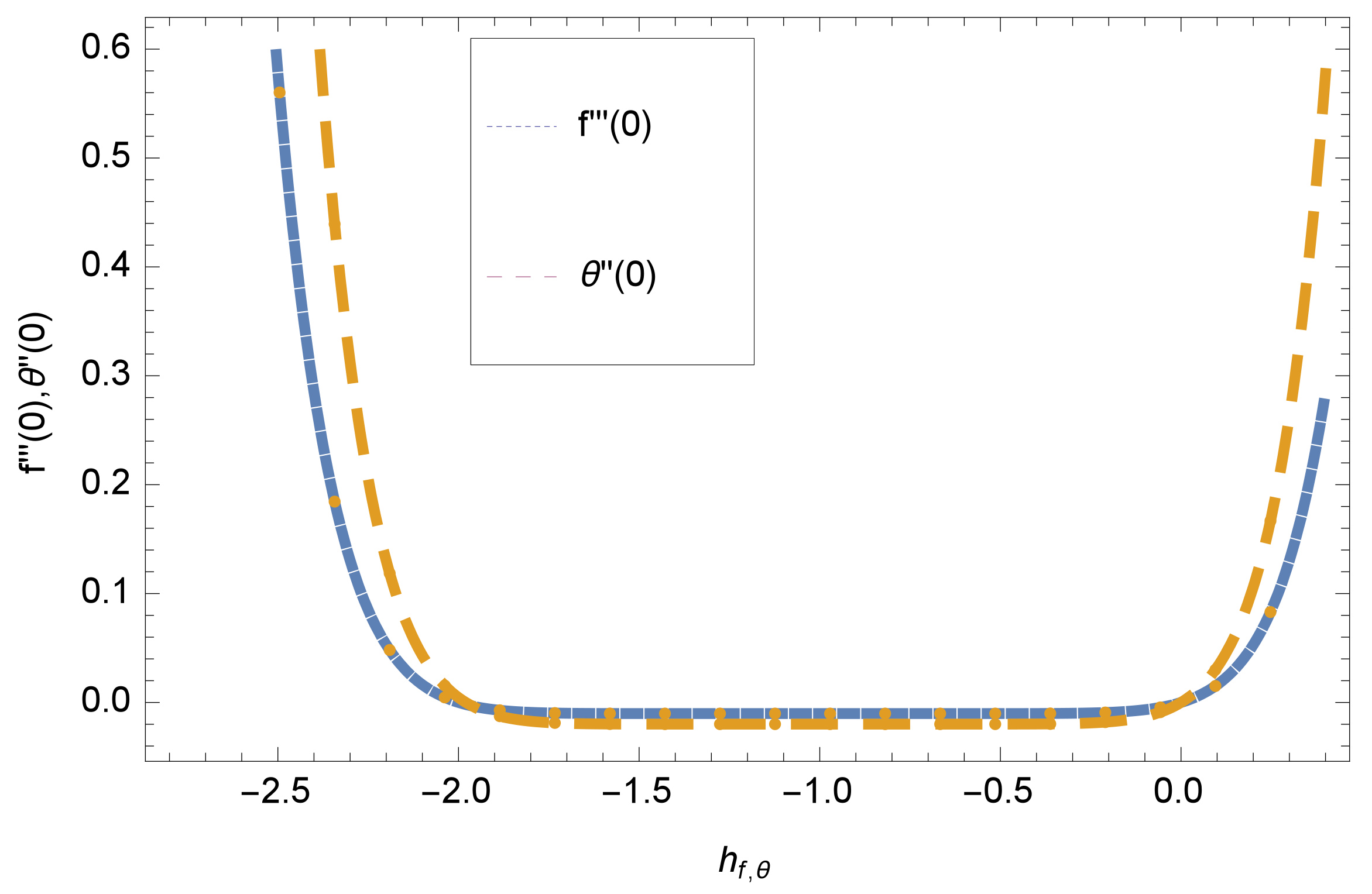
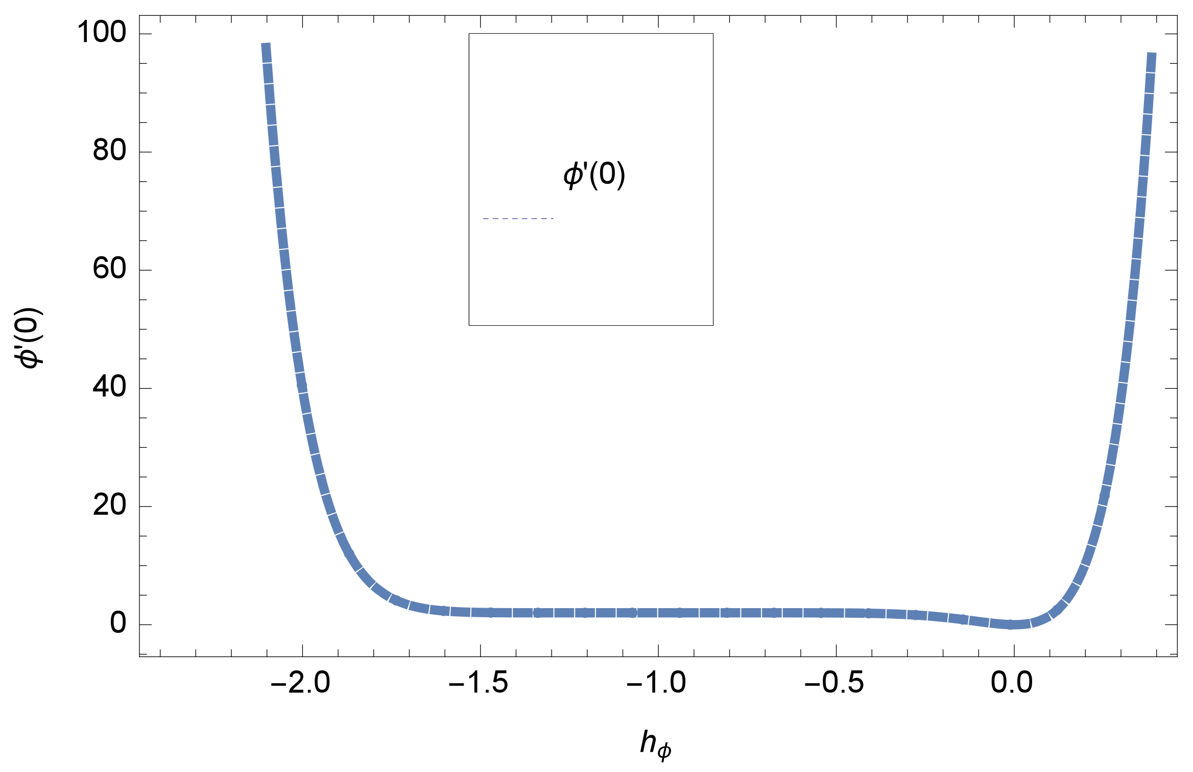
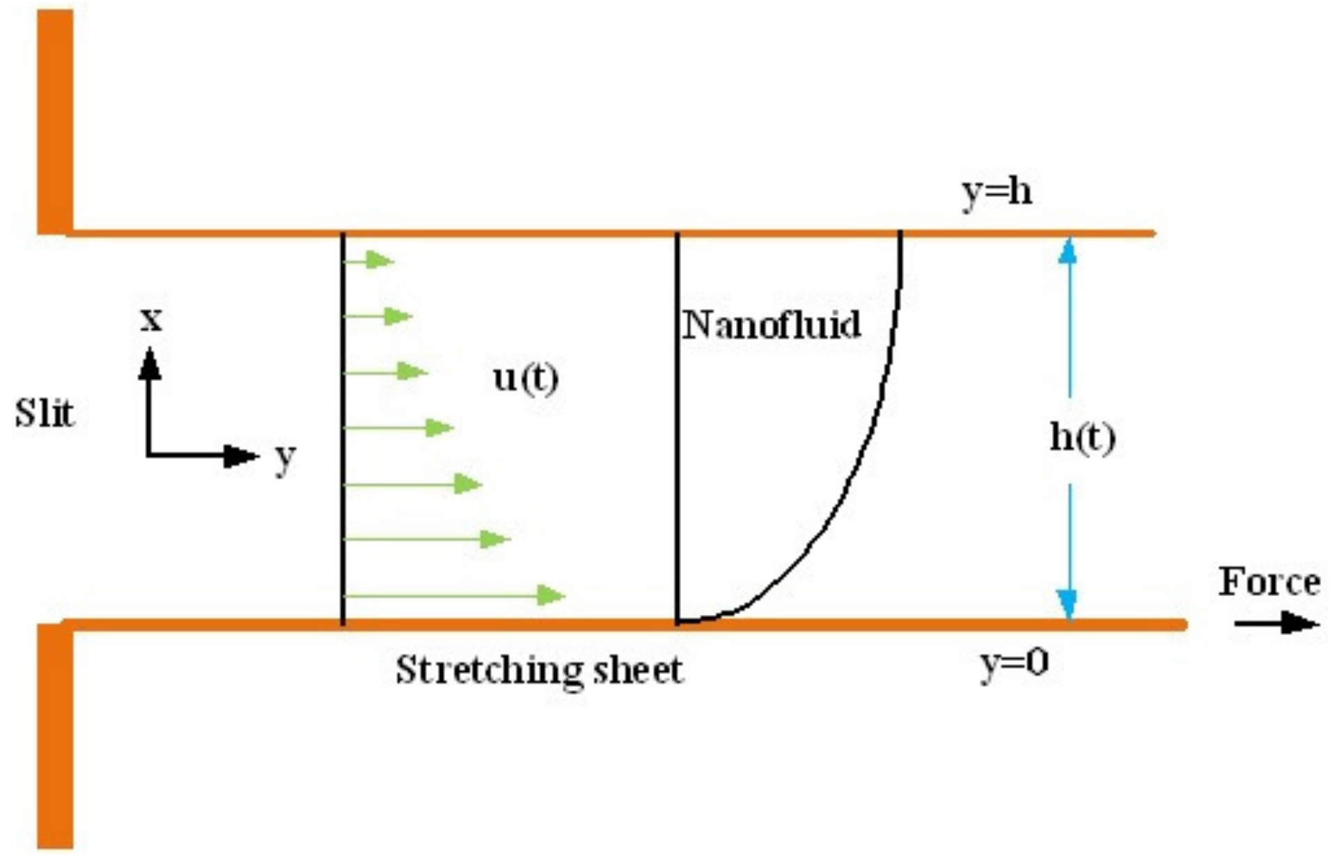
Figure 3 shows the physical model of the problem. The graphs of h-curve for different order Approximation are plotted in
Figure 1 and
Figure 2 for various values of embedded variables. The h-curves consecutively display the valid region. In particular, we discuss the influence of various embedded parameters on velocity profile, temperature profile, nanoparticle concentration profile, and entropy profile. The graphical explanation of these parameters has been displayed in figures [
4,
5,
6,
7,
8,
9,
10,
11,
12,
13,
14,
15,
16,
17,
18,
19,
20,
21,
22,
23,
24,
25,
26,
27,
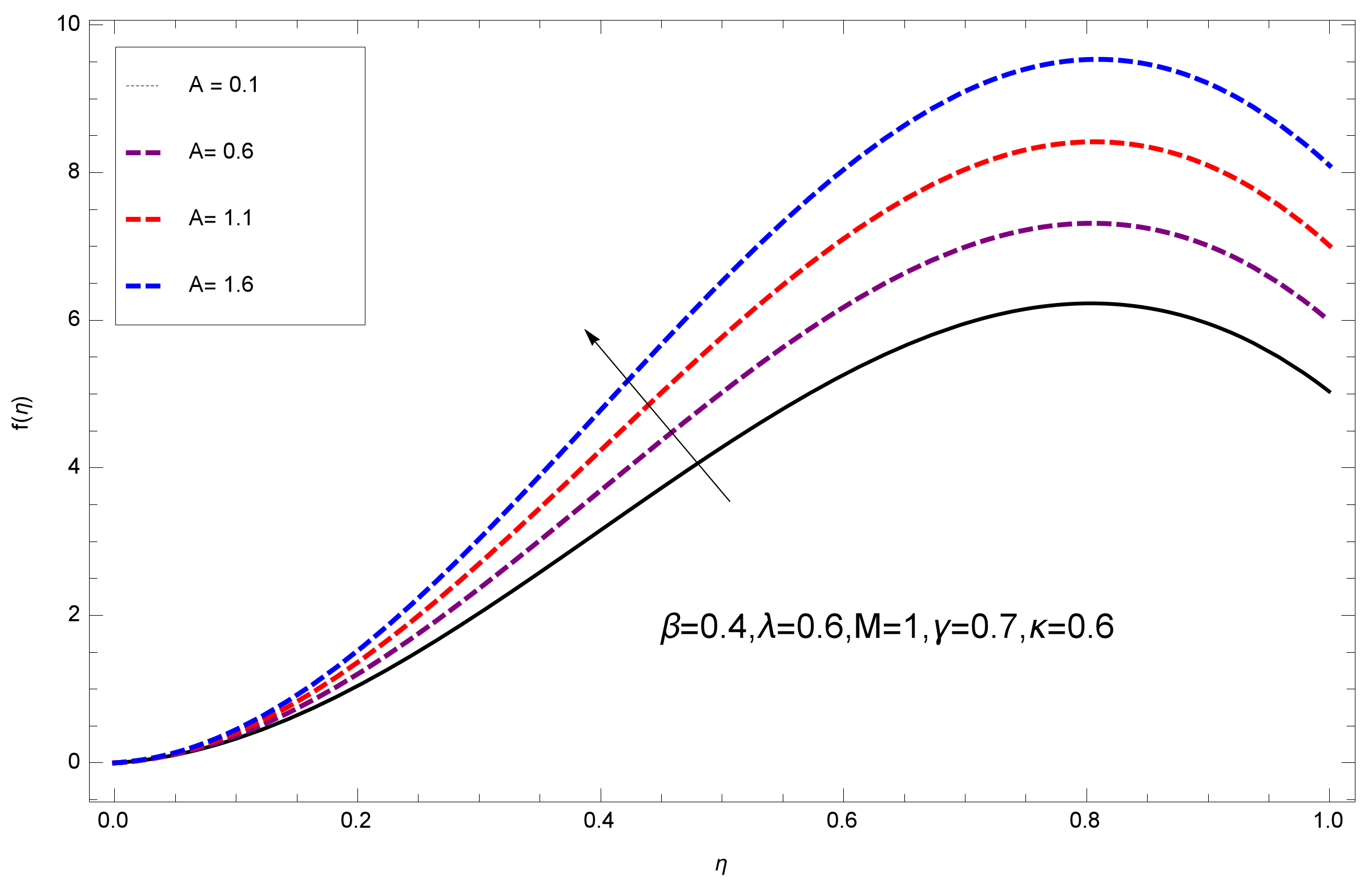
28]. The influence of unsteady constraint
A on the
profile illustrated in
Figure 4. The velocity field
rises with the rise in unsteady parameter
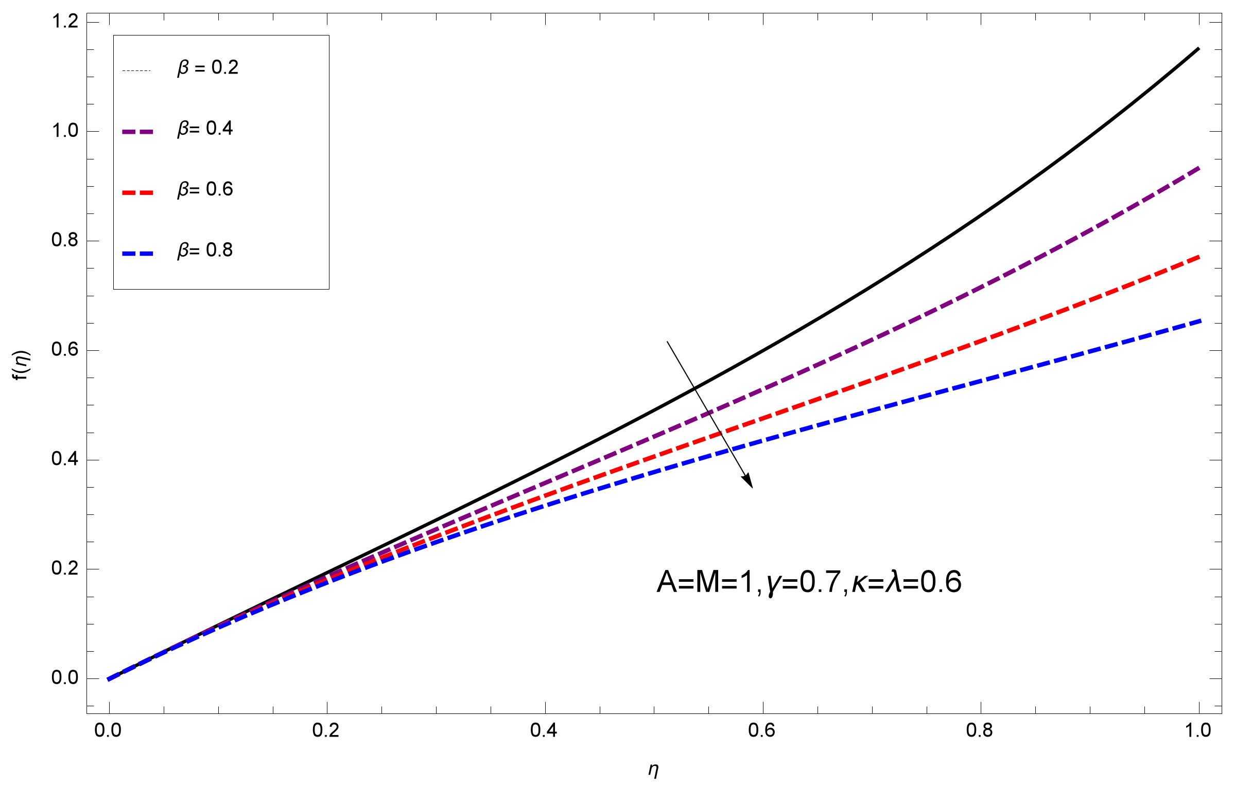
A. The effect of film thickness
has been demonstrated for various values of fluid velocity mentioned in
Figure 5. It is seen that
falls over with higher values of
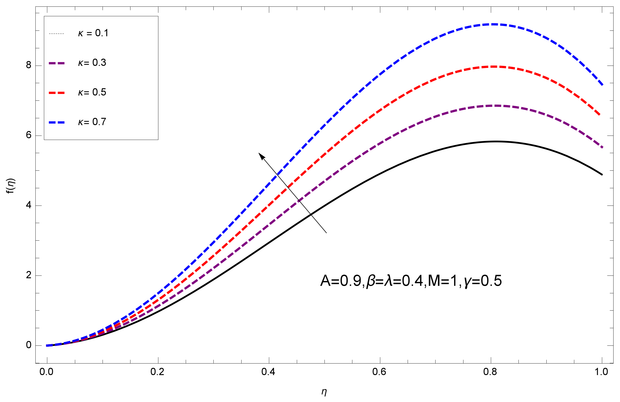
.The impact of Erying fluid factor
k over the
is exposed in
Figure 6. It has been observed that, when Erying fluid parameter
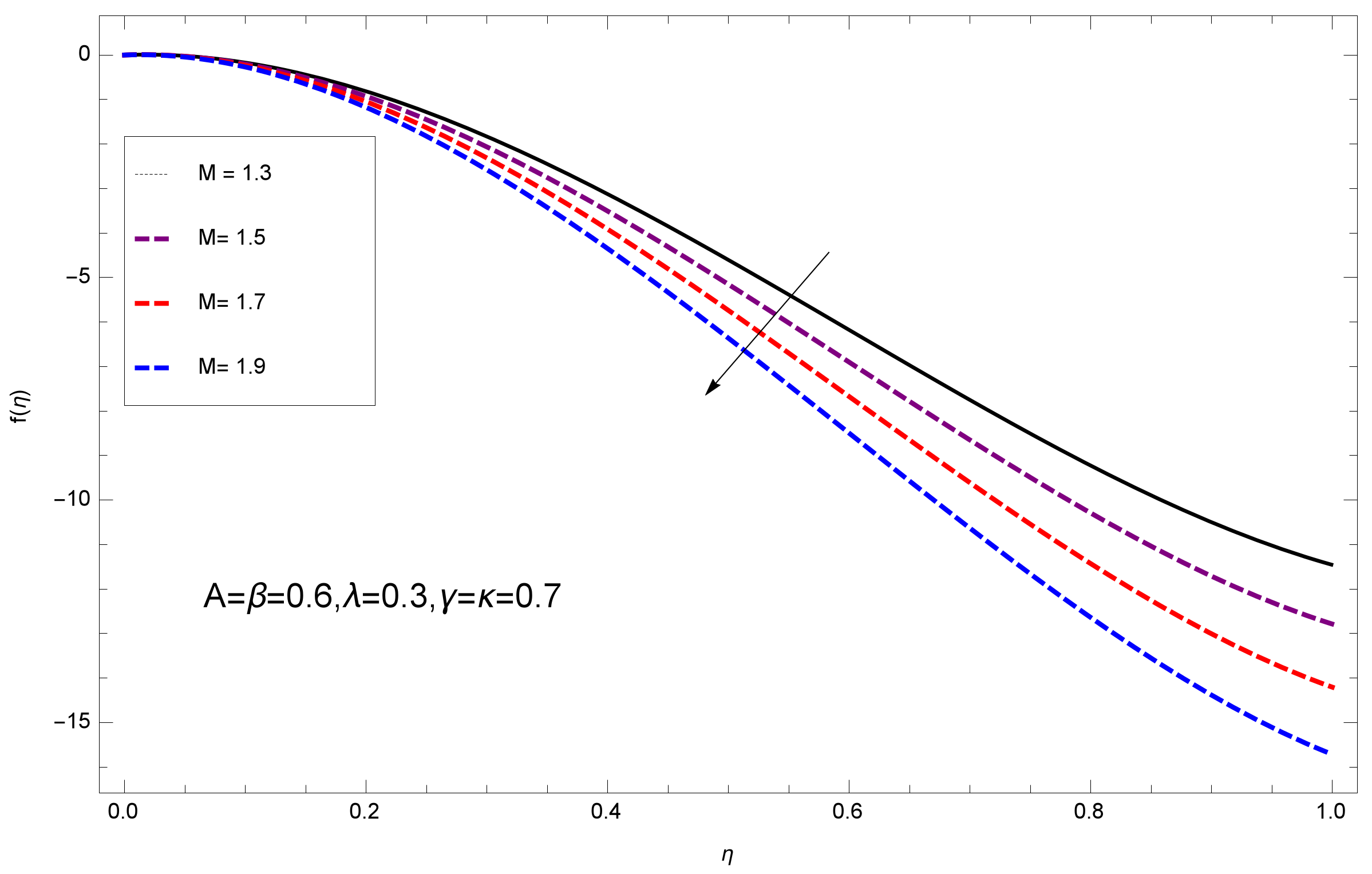
k increases, then it raises the nanofluid film motion, and this effect is clear at the stretching surface. The characteristics of magnetic factor
M on fluid velocity profile is shown in
Figure 7. It is obvious from mathematical formulation that the magnetic parameter
M is inversely varied with velocity distribution
. Increasing magnetic parameter
M decreases the velocity field. This influence of magnetic field is caused by the production of friction force to the movement known as the Lorentz force, which brings retardation to the flow of the fluid and hence reduces fluid velocity at the edge.The characteristics of porosity parameter
on velocity field is shown in
Figure 8, which have an imperative character in the flow motion. Increasing
increases the porous space which creates resistance in the flow path and reduces the flow motion. In fact, growing values of
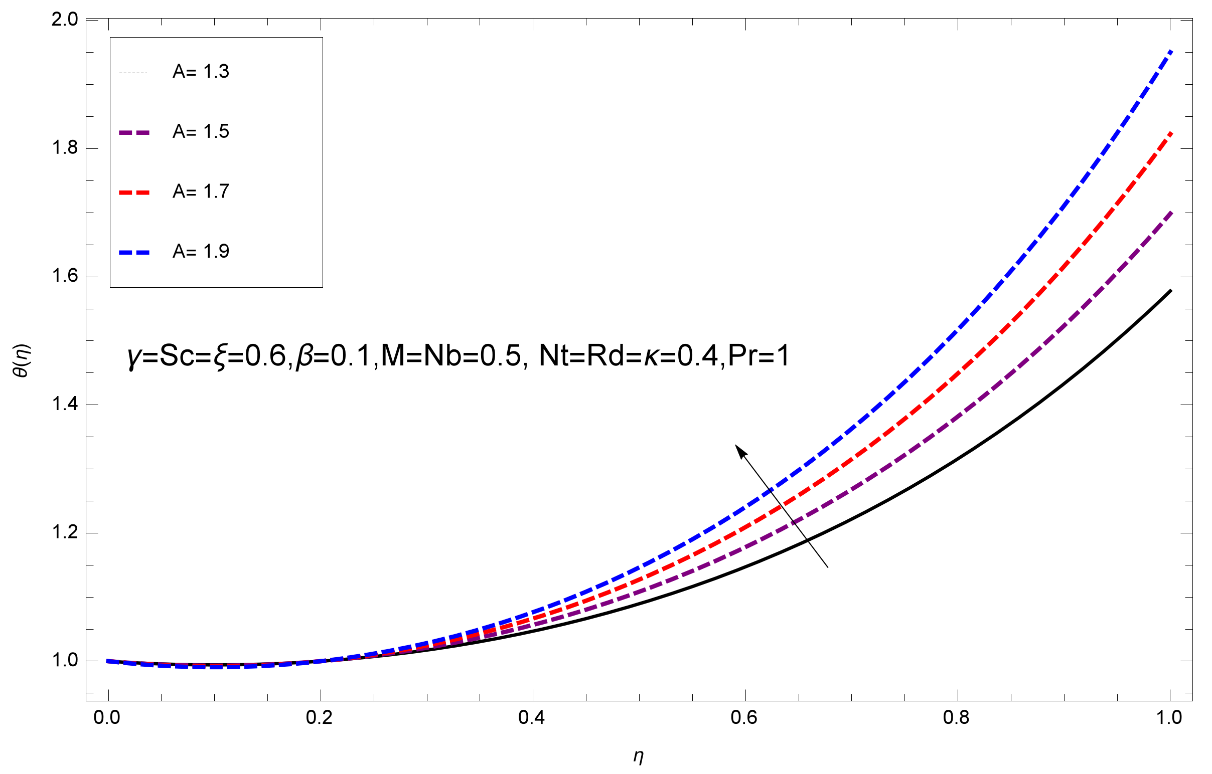
show the large number of porous spaces, which create resistance in the flow path and reduce overall fluid motion. Basically, with the increaseing number of holes in the porous plates the nanoliquid particles face hurdles in flow over these holes. Throughout this motion the way is not clear and the fluid has to decrease its velocity at any point. The unsteady parameter
A has an opposite effect on temperature profile.
Figure 9 depicts that temperature depreciates with the unsteady parameter
A. Each and every fluid has the similar effect on temperature for the unsteady parameter
A. The fluid produces confrontation to the flow of film and shows a tendency to reduce the velocity of fluid flow having larger values of
and it is clear in
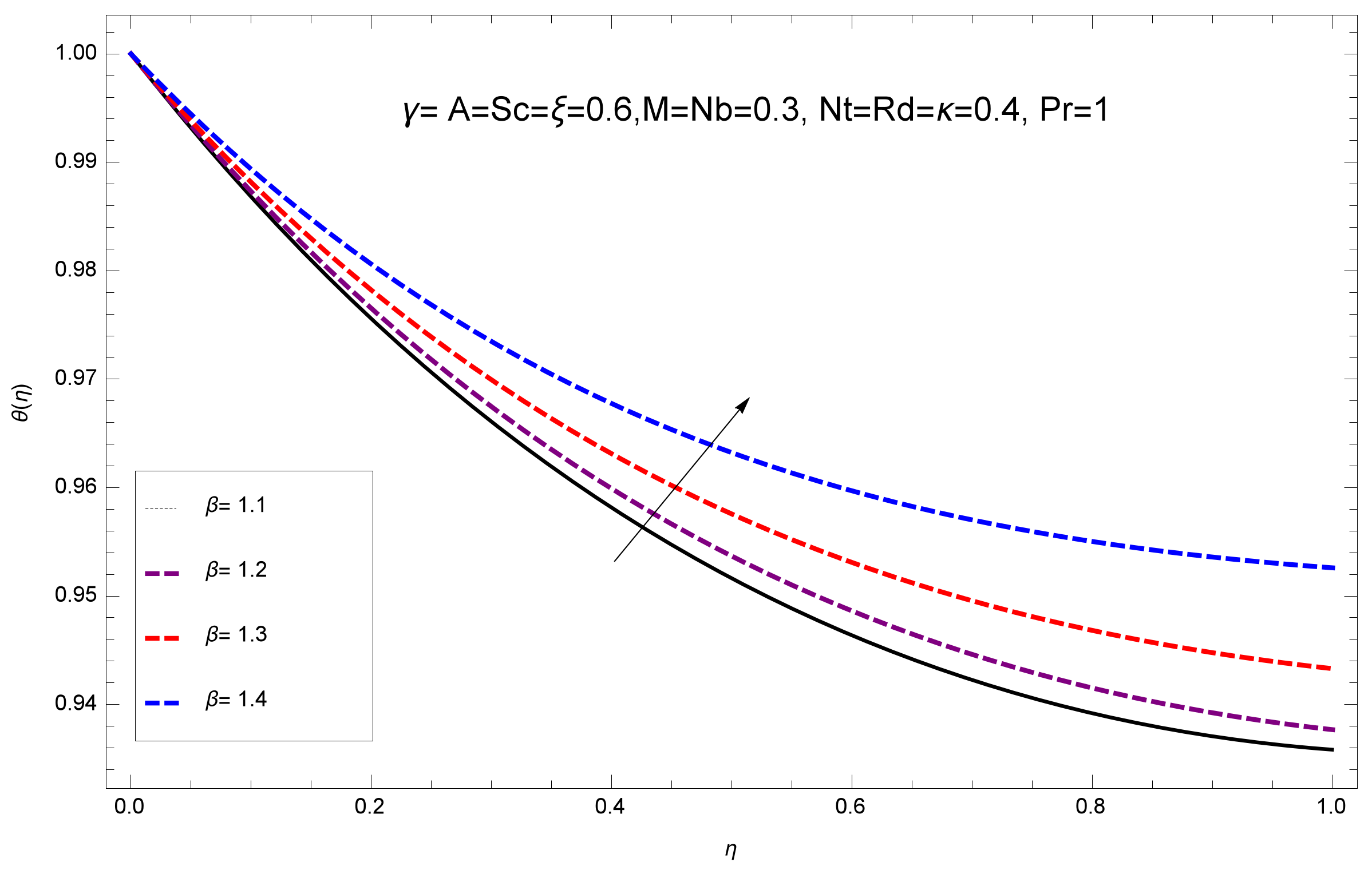
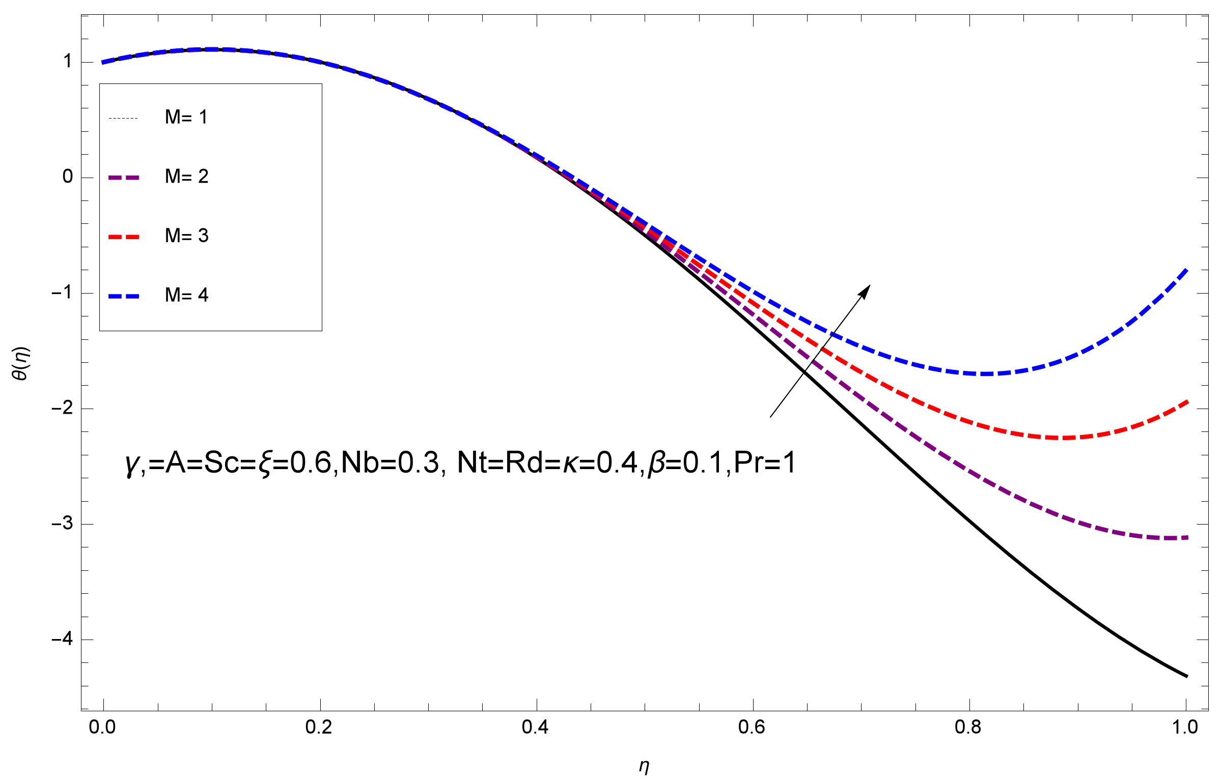
Figure 10. The fluid film size absorbs heat that causes fall down in temperature distribution. The characteristics of magnetic factor
M on temperature profile is shown in
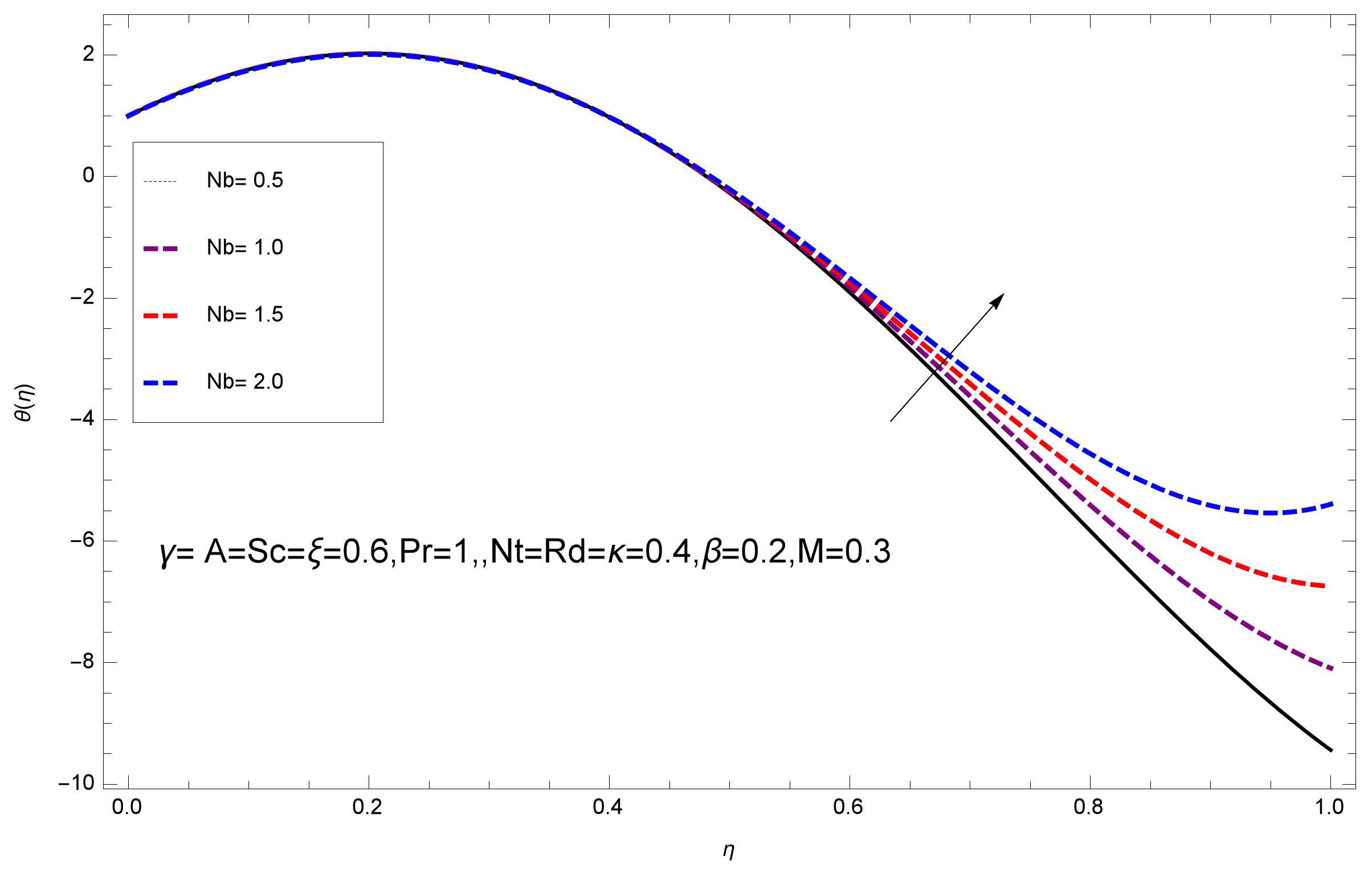
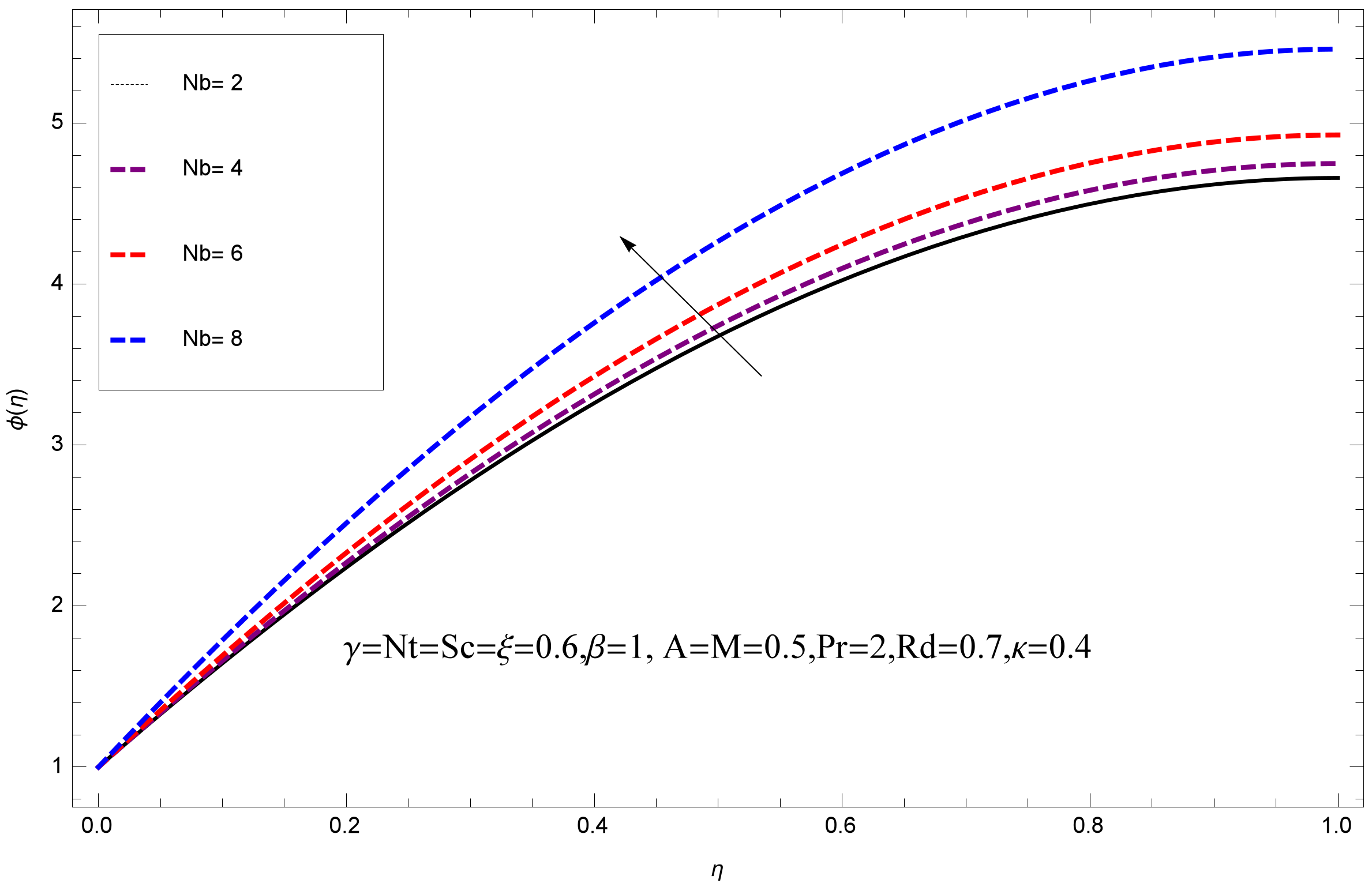
Figure 11. The steepness in the temperature profiles decreases with decreasing the width of the thermal boundary layers. The free surface temperature is increased with the Brownian motion constraint as illustrated in
Figure 12. Actually, Brownian motion is the erratic random movement of microscopic particles in a fluid, as a result of continuous bombardment from molecules of the surrounding medium. The reality is that arbitrary motion of particles of the fluid generates collision in the particles. Increase in the value of Brownian motion constraint
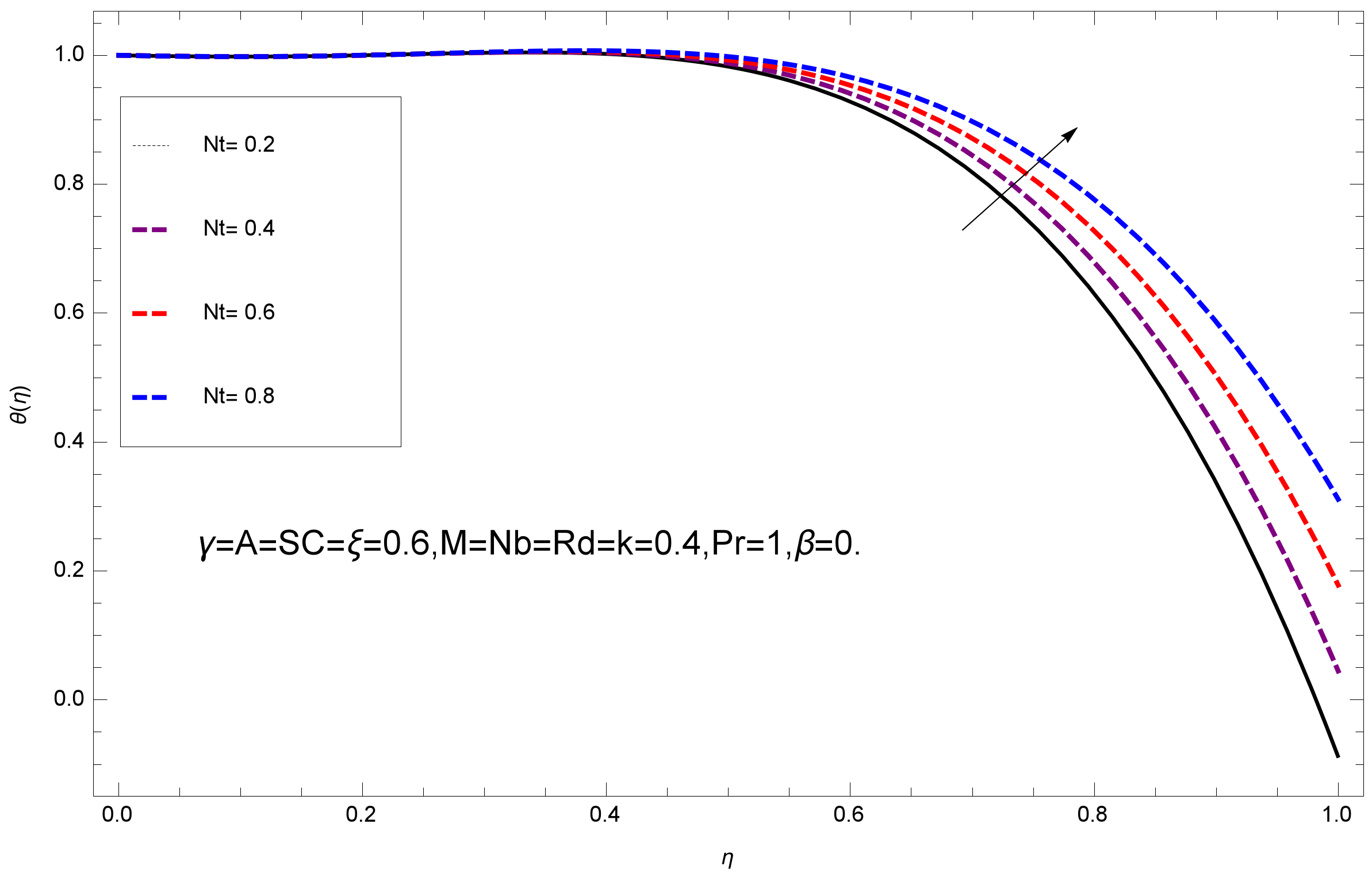
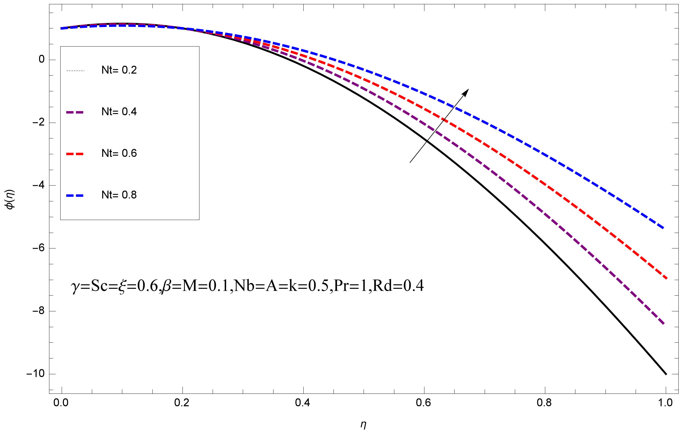
results in an increase in temperature of the fluid. Consequently, it causes reduction in free surface nanoparticle volume fraction. Due to kinetic molecular theory, the heat of the fluid increases due to the increase of Brownian motion. Thus, the given result is in good agreement with the real situation. The thermophoresis parameter
faces depreciation in contrast with temperature profile. This phenomenon is described by
Figure 13. The thermophoresis limitation supports growing the surface temperature. The irregular moment of nano suspended particles in the fluid represented the Brownian motion. Due to this irregularity in motion, nano suspended particles produce kinetic energy and the temperature increases; as a result, the thermophoretic force is initiated. This force causes intensity in the fluid to move away from the surface of the stretching sheet. Subsequently, the temperature inside the boundary layer rises as
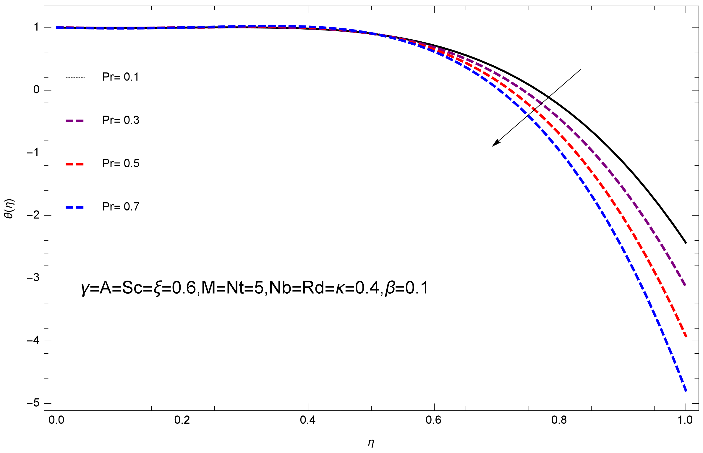
grows.Physically, Prandtl number is the ratio of kinematic viscidness to thermal diffusivity and is a dimensionless quantity. The
is increased when the value of momentum diffusivity is greater than the thermal diffusivity. Thus, heat transmission at the surface grows with the increase in
values while mass transmission is concentrated as the Prandtl number grows. The impact of
is given in the
Figure 14. It clearly shows that
reduces with large
number. The logic behind this is that, with the large value of
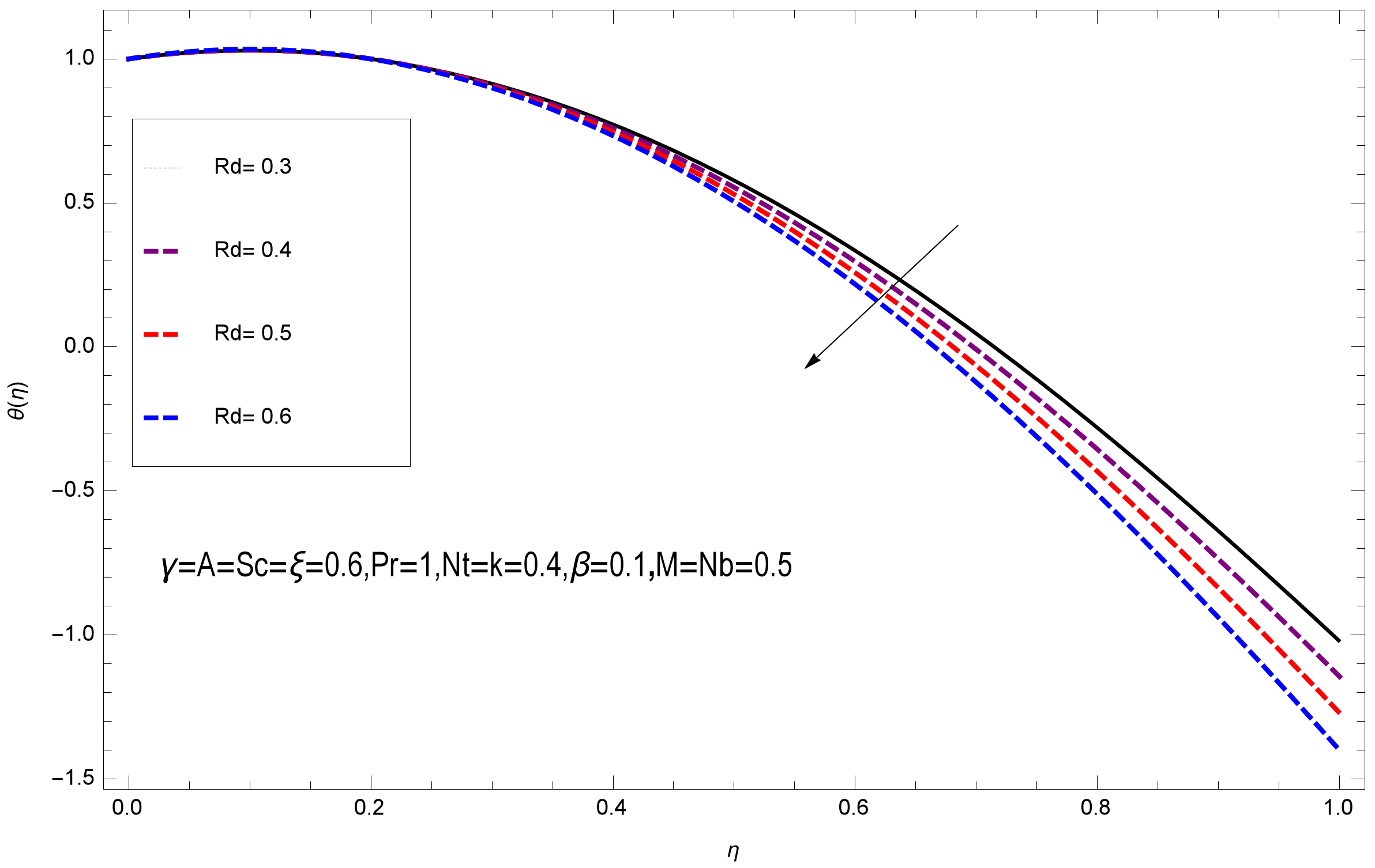
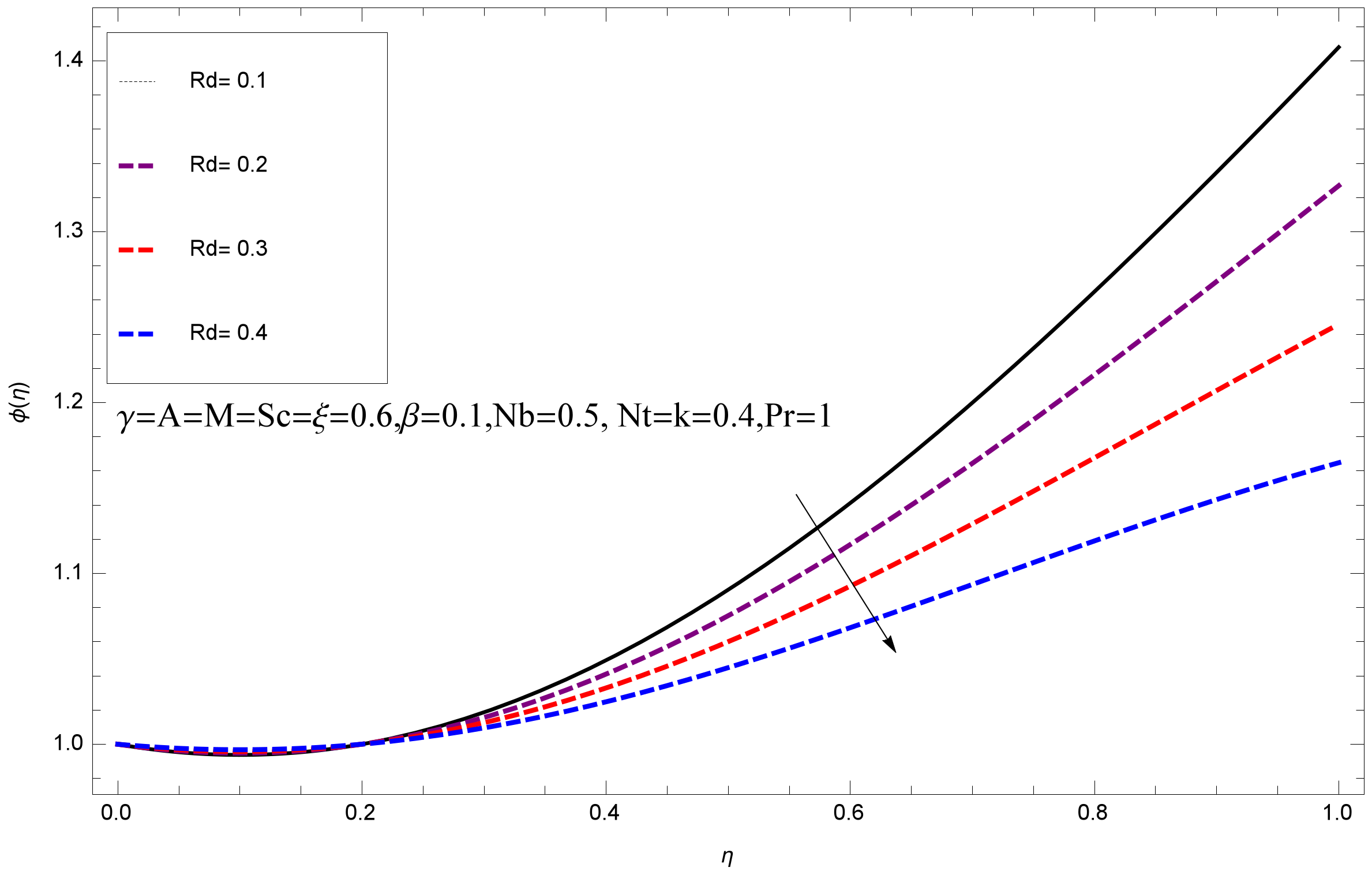
, thermal layer of the boundary reduces. The consequence is more noticeable for slight Prandtl quantity as the width of the thermal boundary layer is relatively greater. The influence of
parameter on temperature is presented in
Figure 15. Thermal radiation has an imperative part in inclusive surface heat transmission when the coefficient of convection heat transmission is small. When we increase the value of
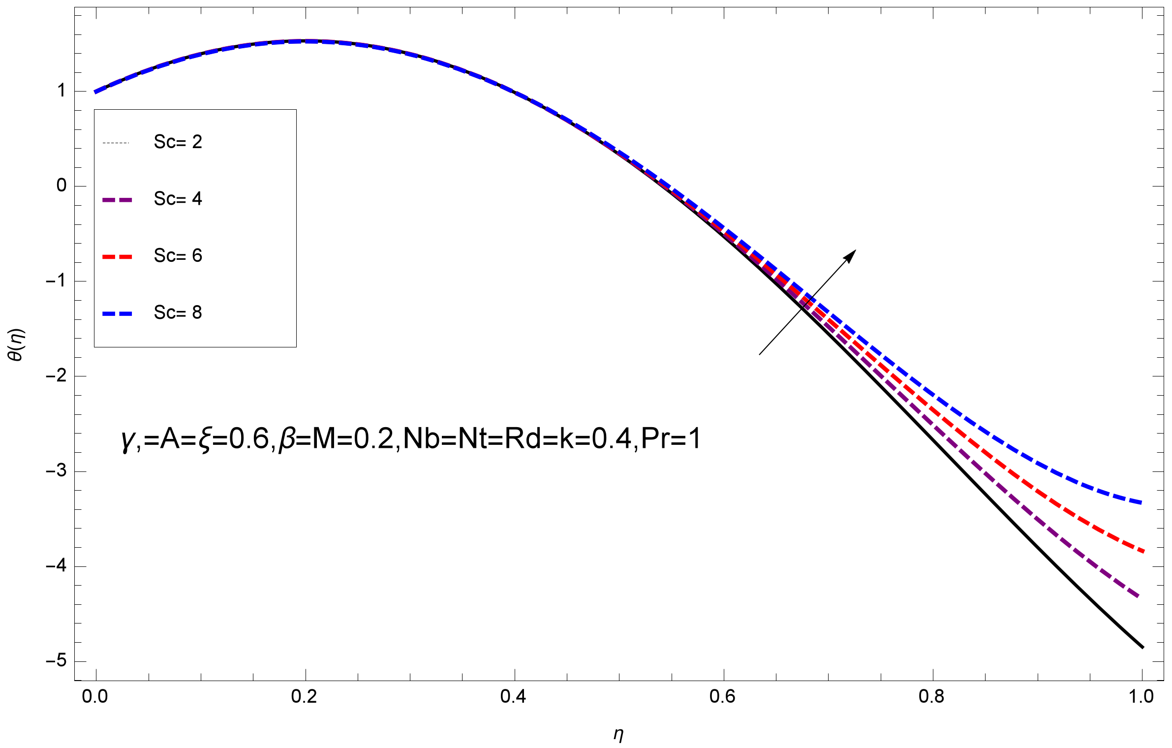
, it is perceived that it augments the heat in the boundary layer of the fluid. This increase causes a drop in the rate of cooling in nanofluid flow. The heat field
increases with the change in the Schmidt number illustrated in
Figure 16. It is obvious that the flow part increases in the horizontal direction by giving rise in the Schmidt number. It is trivial that, with a rise in the Schmidt number, the flow part increases in the
x-direction. The logic behind is that the Schmidt parameter is the ratio of momentum and concentration diffusivities. The rise in the values of
decreases width of the fluid and causes fall down in
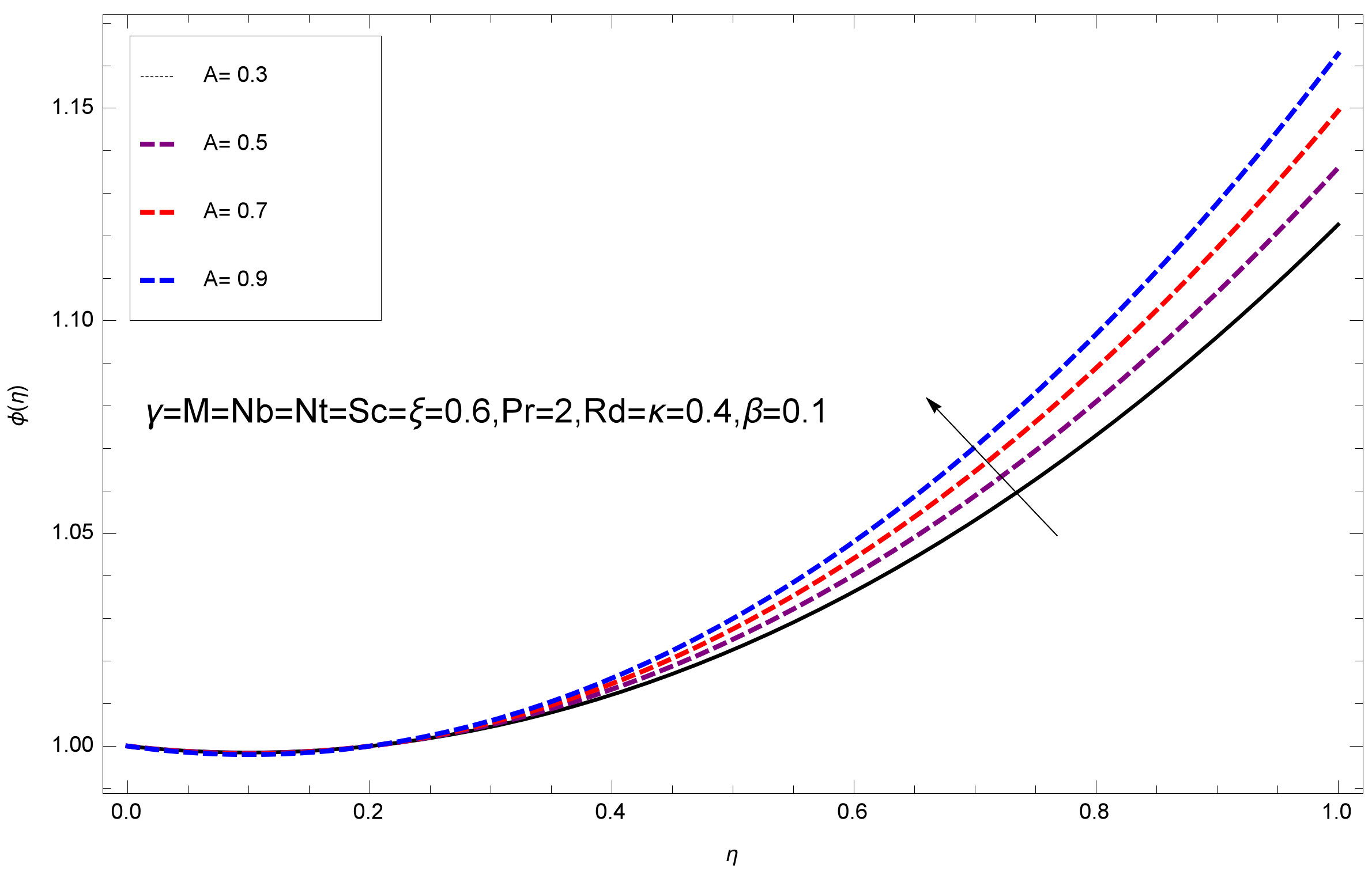
. It is obvious from
Figure 17 that the increasing values of unsteady parameter A increases the concentration profile
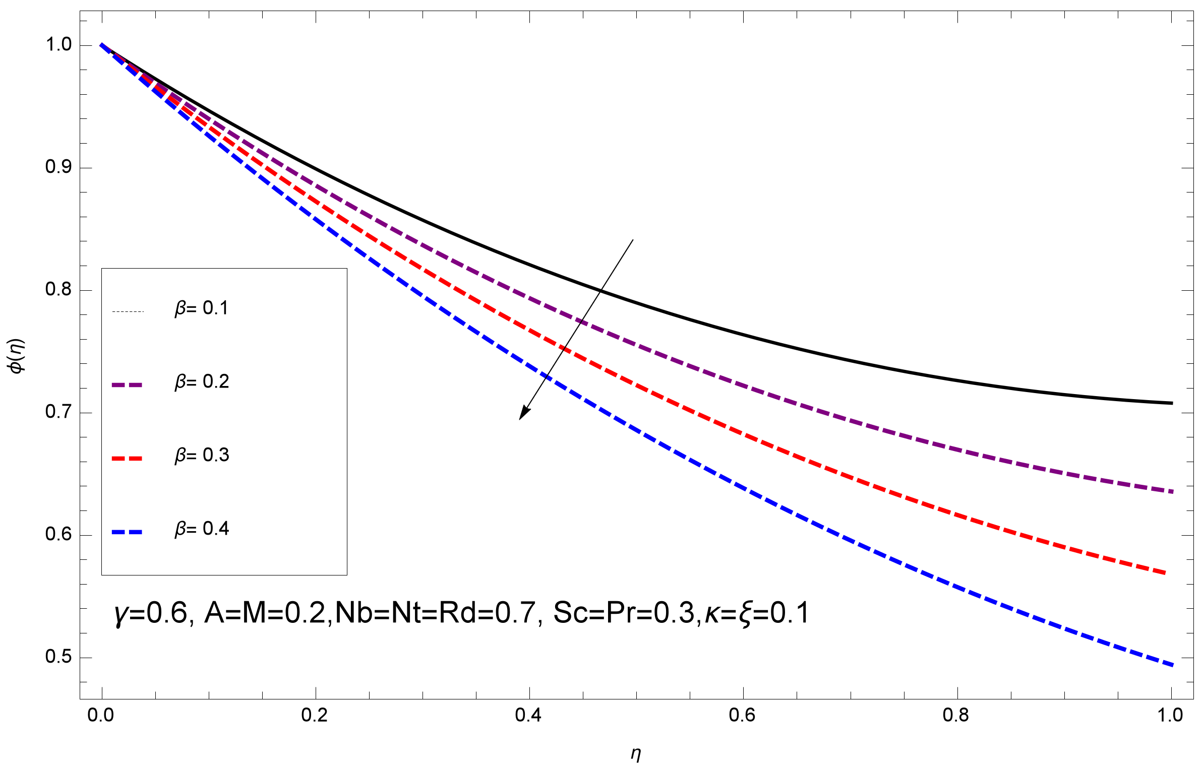
. The concentration of the fluid
rises as values of
progress, as exhibited by
Figure 18. The logic behind this is that the fluid film width exhibits a direct relation with thermal conductivity and viscosity. The impact of varying
parameter with respect to the concentration profile
on domain
has an increasing impact of
and has been observed for both suction and injection, and it is displayed in
Figure 19. As thermophoresis parameter
rises, elevation occurs in the concentration profile. Thermophoresis restriction also helps in rising the surface nano particle volume fraction like the surface temperature shown in
Figure 20. The surface mass transfer rate in steady and unsteady cases decreases with increasing the thermophoresis factor
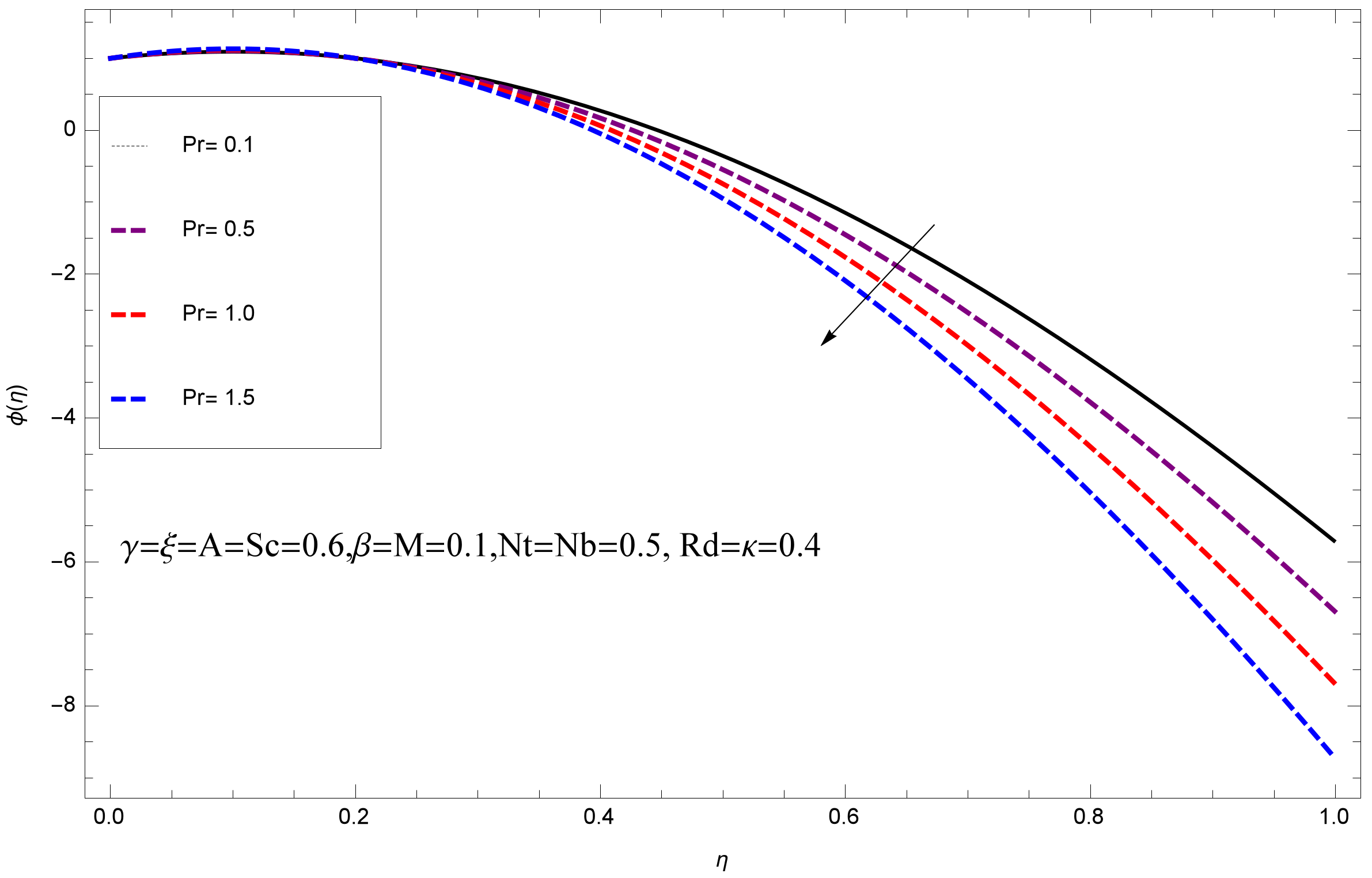
, but show high surface mass transfer rate in unsteady cases as compared to steady ones. Concentration profile exhibits the inverse relation with
number shown in
Figure 21. It means that thinning of the thermal boundary layer progresses the flow in the
x-direction, which is reflected in the graph. The influence of
parameter on concentration profile is presented in
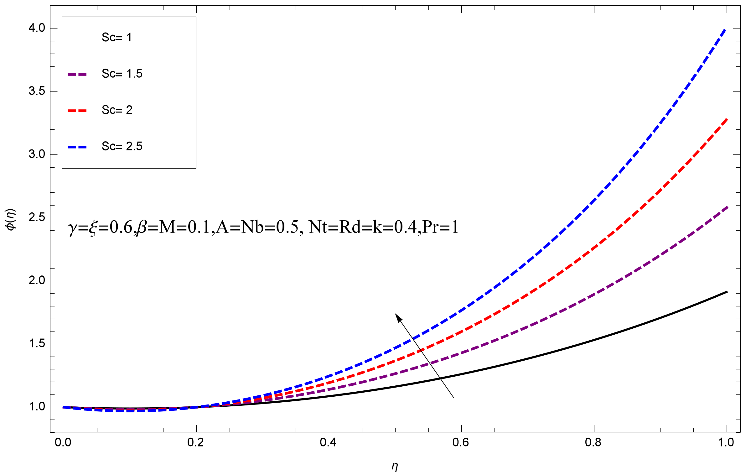
Figure 22. When we increase the value of
, it is perceived that it augments the concentration in the boundary layer of the fluid. This increase causes a drop in the rate of cooling in nanofluid flow. The non-dimensional concentration profile reduces with dissimilar measures of parameter
shown in
Figure 23. It is obvious that a flow part increases in the horizontal direction by giving rise in the Schmidt number. It is trivial that, with a rise in the Schmidt number, the flow part increases in the
x-direction. The logic behind is that the Schmidt parameter is the ratio of momentum and concentration diffusivities. The viscidness dissipation effect on the nanoparticle volume fraction is insignificant for higher quantities of Schmidt numbers.
Figure 24,
Figure 25,
Figure 26,
Figure 27 and
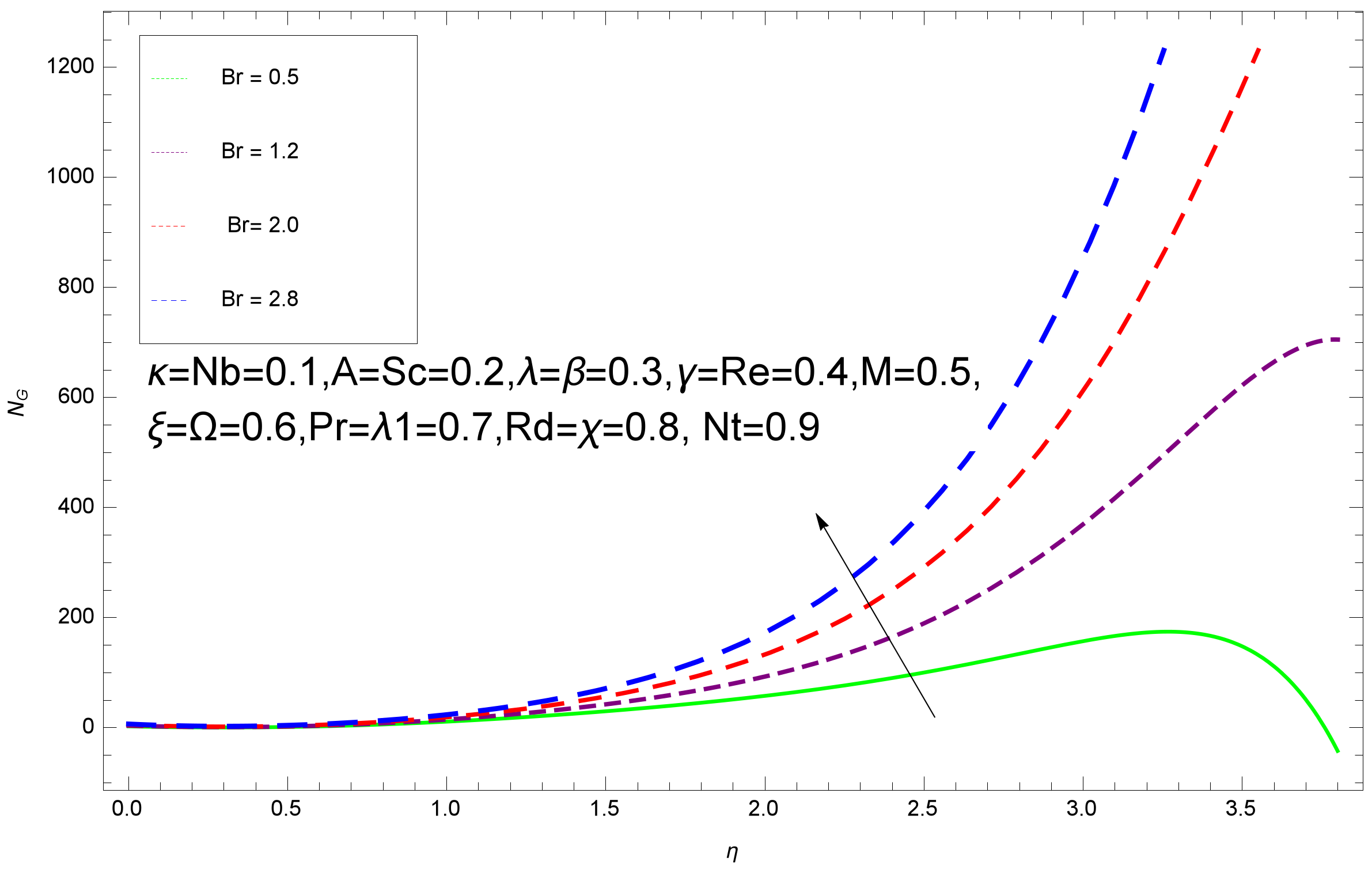
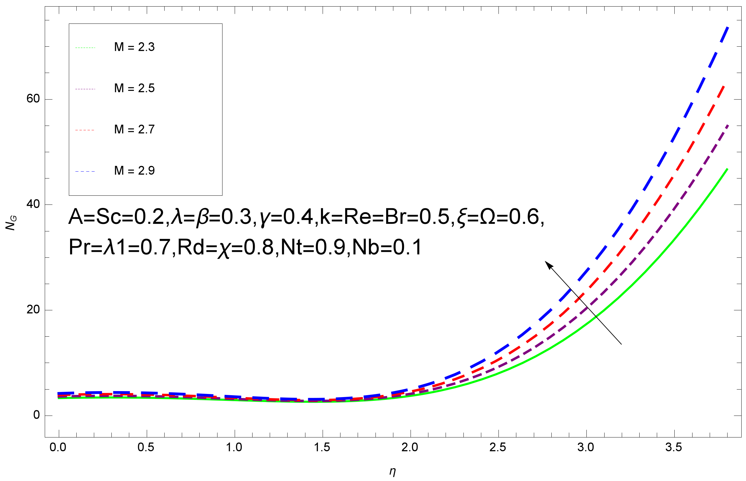
Figure 28 represent the entropy profile for the Brinkmann
, Eyring–Powell parameter
k, Magnetic parameter
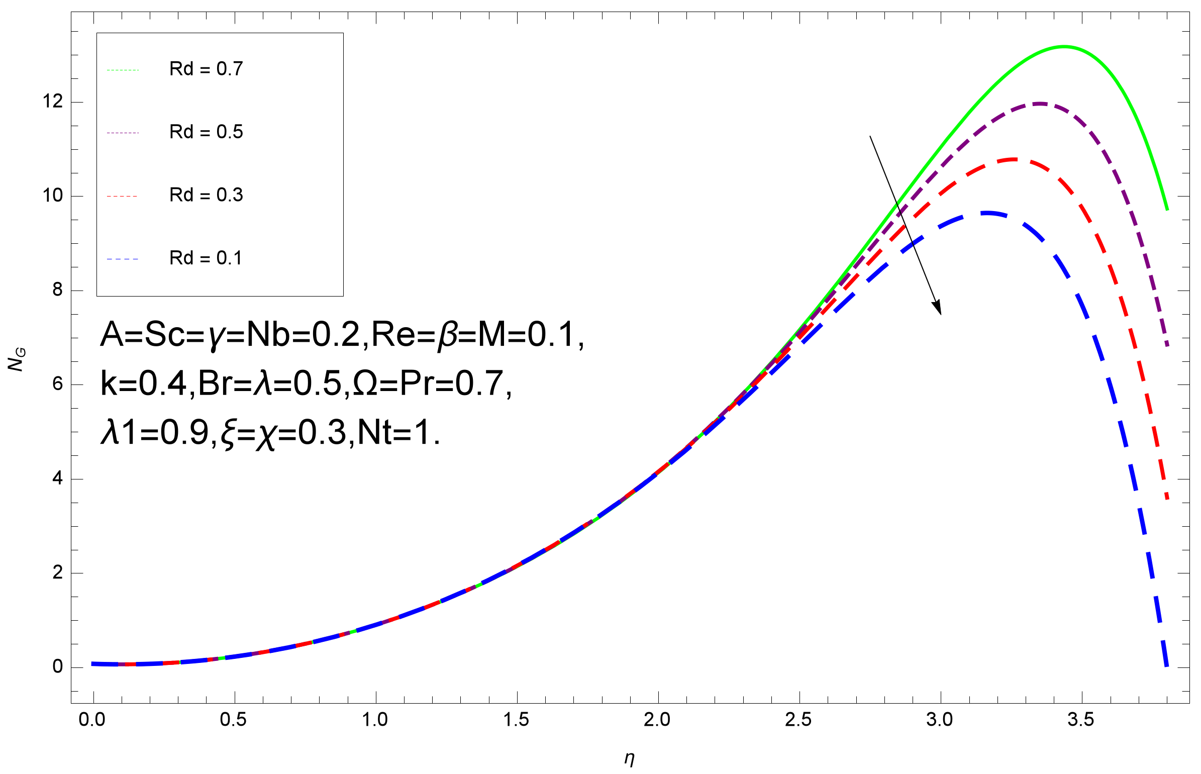
M, Radiation parameter
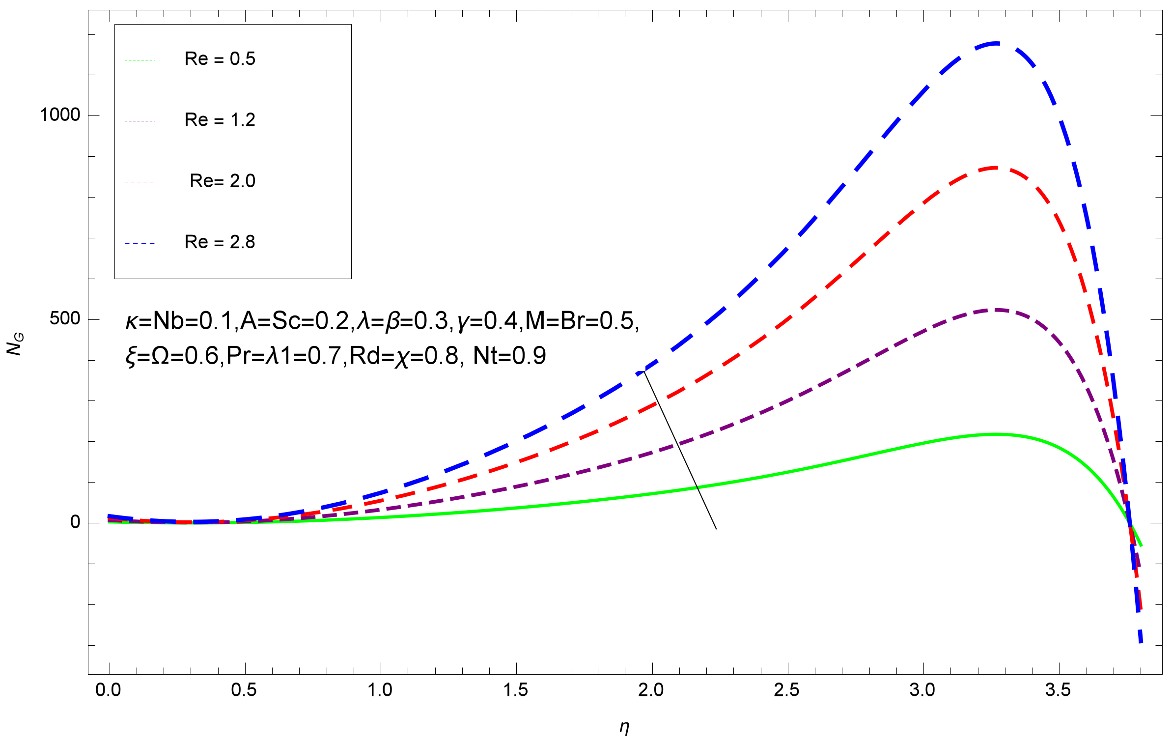
and Reynolds number
. It is clear from
Figure 24,
Figure 26 and
Figure 28 that the entropy profile increases due to increase in
,
M, and
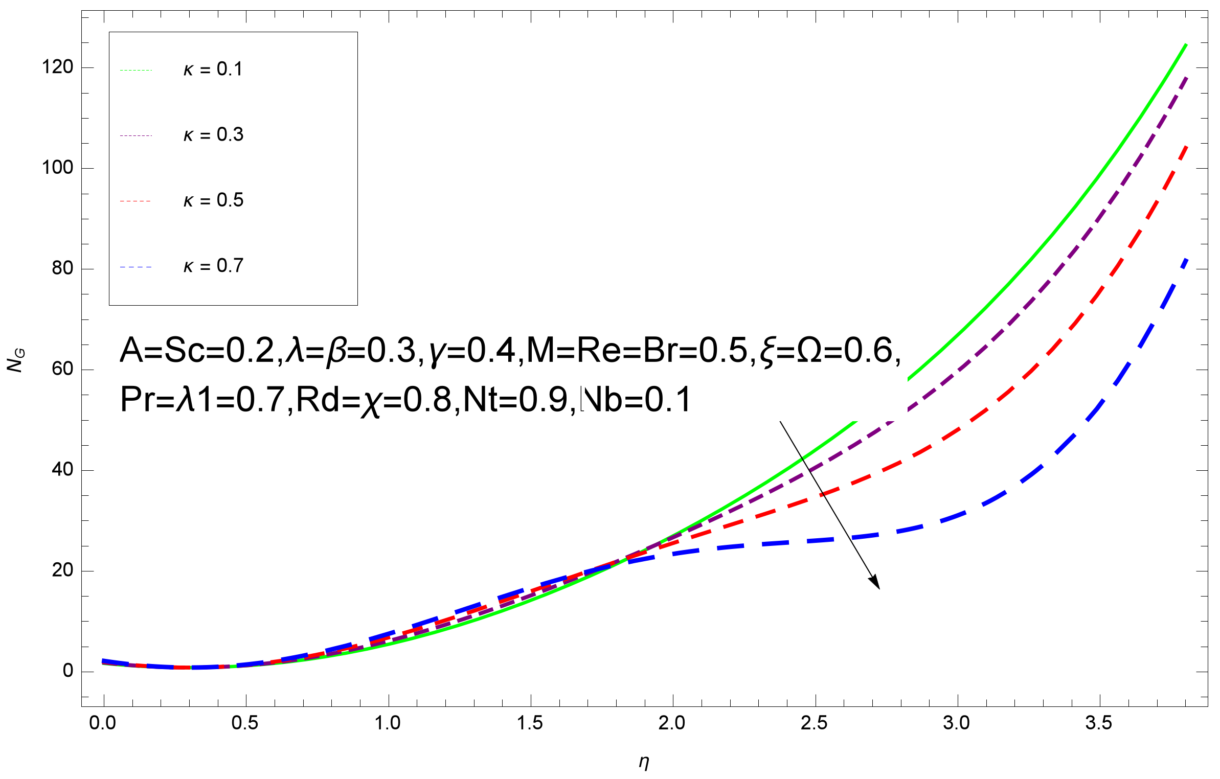
, respectively. On the other hand, it is reflected from
Figure 25 and
Figure 27 that the entropy generation field decreases with increasing values of parameter
k and
.


