A Chaotic Electromagnetic Field Optimization Algorithm Based on Fuzzy Entropy for Multilevel Thresholding Color Image Segmentation


College of Mechanical and Electrical Engineering, Northeast Forestry University, Harbin 150040, China
*
Author to whom correspondence should be addressed.
Entropy 2019, 21(4), 398; https://doi.org/10.3390/e21040398
Submission received: 1 April 2019
/
Revised: 11 April 2019
/
Accepted: 12 April 2019
/
Published: 15 April 2019
(This article belongs to the Special Issue Entropy in Image Analysis)
Abstract
:Multilevel thresholding segmentation of color images is an important technology in various applications which has received more attention in recent years. The process of determining the optimal threshold values in the case of traditional methods is time-consuming. In order to mitigate the above problem, meta-heuristic algorithms have been employed in this field for searching the optima during the past few years. In this paper, an effective technique of Electromagnetic Field Optimization (EFO) algorithm based on a fuzzy entropy criterion is proposed, and in addition, a novel chaotic strategy is embedded into EFO to develop a new algorithm named CEFO. To evaluate the robustness of the proposed algorithm, other competitive algorithms such as Artificial Bee Colony (ABC), Bat Algorithm (BA), Wind Driven Optimization (WDO), and Bird Swarm Algorithm (BSA) are compared using fuzzy entropy as the fitness function. Furthermore, the proposed segmentation method is also compared with the most widely used approaches of Otsu’s variance and Kapur’s entropy to verify its segmentation accuracy and efficiency. Experiments are conducted on ten Berkeley benchmark images and the simulation results are presented in terms of peak signal to noise ratio (PSNR), mean structural similarity (MSSIM), feature similarity (FSIM), and computational time (CPU Time) at different threshold levels of 4, 6, 8, and 10 for each test image. A series of experiments can significantly demonstrate the superior performance of the proposed technique, which can deal with multilevel thresholding color image segmentation excellently.
1. Introduction
Image segmentation is an important technology in image processing, which is a frontier research direction in computer vision, as well as one of the key preprocessing steps in image analysis [1,2]. It has been widely adopted in medicine, agriculture, industrial production, and various other fields. Image segmentation can be defined as the procedure of dividing an image into different regions [3]. In the subsequent research, the relevant regions can be extracted from the segmented image expediently according to specific requirements. Nowadays, the common image segmentation methods include threshold-based, cluster-based, edge-based methods and so on. Thresholding is extensively applied due to its simplicity, efficiency, and robustness. Depending on the number of thresholds, it can be classified as bi-level segmentation and multilevel segmentation [4]. Bi-level thresholding techniques use one threshold to partition an image into two segments; whereas multilevel segmentation determines several thresholds to separate an image into more than two classes. Many thresholding approaches have been proposed by scholars around the world in the past few years, Otsu’s (between-class variance criterion) [5,6] technique pushes the thresholding segmentation to an upsurge and inspires the scholars constantly in this field. Then diverse entropy-based criteria have emerged in the thresholding segmentation study, such as maximum entropy (Kapur’s) [7], minimum cross entropy [8], fuzzy entropy [9], etc.
Gray-scale image thresholding technology is relatively popular and mature. Compared with the segmentation of gray-scale images, color image segmentation plays a more beneficial role in practical applications, which separates an image into several disjoint and homogenous components based on the information of texture, color or histogram [10]. Color image segmentation is more complex and challenging than gray-scale images. Nevertheless, considering that color images contain more characteristics and they are closer to human visual effects [11], the research of color image segmentation is more meaningful. There will appear some problems when a traditional segmentation method is adopted to segment a color image, for example, the computation is massive and accuracy of segmented images cannot be guaranteed [12,13]. In this paper, fuzzy entropy is one of the research objects with high segmentation accuracy. In the fuzzy entropy thresholding technique, each threshold needs to be determined by three fuzzy parameters. Hence the calculation of thresholds is more accurate, at the same time the process is more complicated and the running time of the program will be longer. With the improvement of the threshold level, the computation of fuzzy entropy will exponentially increase for searching the optimal thresholds and the efficiency of segmentation will gradually decrease [14,15,16]. In order to enhance the practicability of fuzzy entropy thresholding technique, this paper combines fuzzy entropy thresholding with intelligent optimization algorithms to improve the performance with respect to accuracy and efficiency.
Meta-heuristic algorithms are utilized to obtain the optimal solution of the problem [17]. Generally, they are inspired by nature and try to handle the problems from mimicking ethology, biology or physics [18]. For instance, Bird Swarm Algorithm (BSA) [19], Firefly Algorithm (FA) [20], and Flower Pollination Algorithm (FPA) [21] are inspired by ethology or biology; Electromagnetic Optimization (EMO) [22], Wind Driven Optimization (WDO) [23], and Gravitational Search Algorithm (GSA) [24] are inspired by physics. At present, a number of scholars have coupled the optimization algorithms with the field of image segmentation in the literature. For instance, Sowjanya et al. [25] combined a WDO algorithm with Otsu’s method for the segmentation of brain MRI images, it has shown the superior performance in the experiment results. Wasim et al. [26] proposed an improved Bee Algorithm (BA) for multilevel image segmentation, whereby they embedded Levy fight into a Bees Algorithm (the Levy Bees Algorithm, LBA), and the results show that LBA is more stable than BA in this field. Rakoth et al. [27] tried to combine Dragonfly Optimization with Self-Adaptive weight (SADFO) and used SADFO for image segmentation experiments with satisfying results. These references confirm the feasibility of applying optimization algorithms to image thresholding segmentation. However, the above experiments all concentrate on gray-scale images and do not extend the experiments to the analysis of color images. Applying meta-heuristic algorithms to the field of multilevel image segmentation can enhance the convergence speed and efficiency [28]. Therefore, in this paper, Electromagnetic Field Optimization algorithm (EFO) [29] is modified and combined with fuzzy entropy thresholding method to eliminate the complex computation, which is used into the multilevel color image segmentation field for searching the best threshold values.
Electromagnetic Field Optimization is a new meta-heuristic algorithm inspired by the electromagnetic theory developed in physics. EFO algorithm has been applied in several applications, for example, Behnam et al. [30] created a method using EFO for hiding sensitive rules simultaneously, which has fewer lost rules than other well-known algorithms. Bouchekara et al. [31] proposed the optimal coordination of directional overcurrent relays based on EFO, and the results show that EFO is better than other optimization algorithms such as Particle Swarm Optimization (PSO) [32], or the Differential Evolution (DE) algorithm [33], etc. This paper embeds a new chaos strategy into standard EFO algorithm according to the specific problem of color image segmentation named as Chaotic Electromagnetic Field Optimization (CEFO). Employing the CEFO algorithm to optimize the fuzzy parameters which determine the optimal thresholds of an image in fuzzy entropy. To the best of our knowledge, this topic has not been investigated yet. The rest of this paper is organized as follows: in Section 2, the concept of EFO algorithm is elaborated. In Section 3, the chaotic strategy in CEFO algorithm is introduced and explained. In Section 4, the problem definitions and formulas of the Otsu’s, Kapur’s entropy, and the fuzzy entropy are illustrated. In Section 5, the experimental environment is reported. In Section 6, the experimental results and discussions are provided and analyzed. Finally, a brief conclusion of this paper and future works are drawn in Section 7.
2. Electromagnetic Field Optimization
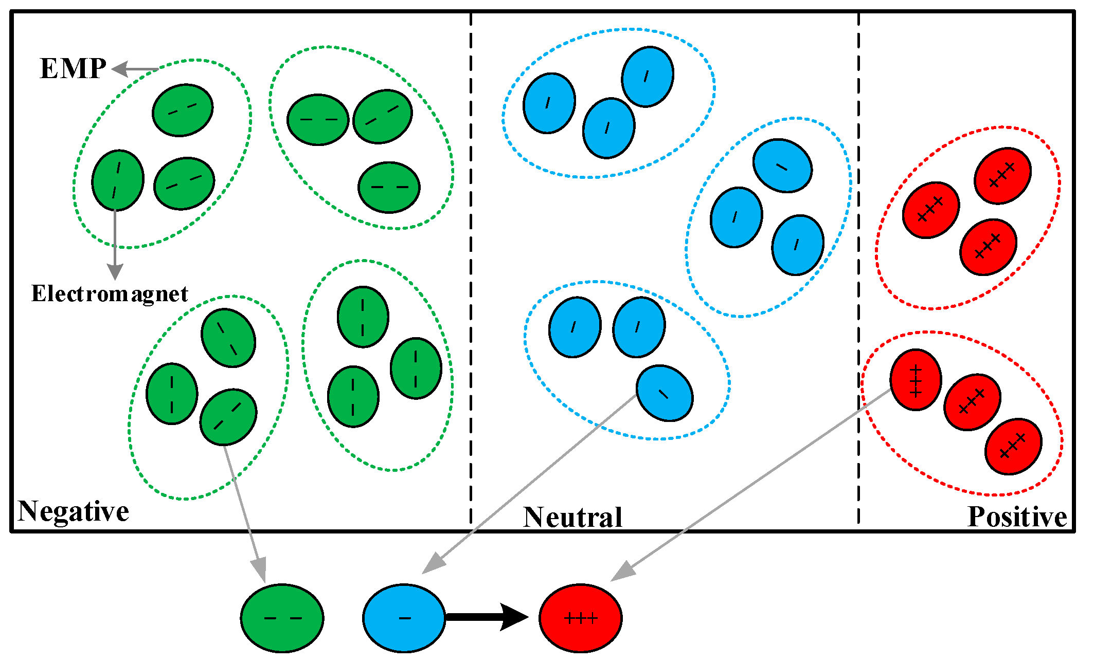
Electromagnetic Field Optimization is a novel meta-heuristic intelligent algorithm proposed by Hosein in 2016 [29]. In contrast to the swarm-based meta-heuristic algorithms widely inspired by biology, the EFO algorithm is based on the electromagnetic field principle used in physics. In the EFO algorithm, due to the forces of attraction and repulsion in the electromagnetic field, the electromagnetic particle (EMP) keeps away from the worst solution and moves towards the best solution. In the end, all the electromagnetic particles (EMPs) gather around the optimal solution.
A magnetic field is generated around the electrified iron core, which is made of an electromagnet. An electromagnet has only one polarity and it is contingent on the direction of the electric current. Hence, an electromagnet has two characteristics of attraction or repulsion, electromagnets with the different polarity attract each other, and those with identical polarity repel each other. The intensity of attraction is 5-10% higher than repulsion and the ratio between attraction and repulsion is set as golden ratio [29,31], which can promote the algorithm to explore the optimal solution effectively in the search space. The essence of the optimization problem is to find the pole (maximum or minimum) about the objective function and the corresponding fitness in the prescriptive range [34]. Each potential solution of the problem is represented with an electromagnetic particle composed of a group of electromagnets. The electromagnetic field comprises several electromagnetic particles and it can be defined as a space in 1-D (dimension), 2-D, 3-D, or hyperdimensional space [35]. The number of electromagnets of an electromagnetic particle corresponds to variables of the optimization problem, as well as the dimension of the electromagnetic space. Moreover, all electromagnets of one electromagnetic particle have the same polarity. Therefore, an electromagnetic particle has the same polarity with its electromagnets. The set of electromagnetic particles can be considered in a matrix as:
where is the number of electromagnetic particles and is the number of variables (dimension).
The mechanism of the EFO algorithm can be described as follows:
- Step 1:
- A certain number of electromagnetic particles are generated randomly in the electromagnetic field, and the fitness of each electromagnetic particle is evaluated by the objective function. Then the electromagnetic particles are sorted on the basis of their fitness.
- Step 2:
- The electromagnetic field is divided into three regions: positive, negative and neutral. Then all electromagnetic particles are classified into these three groups. The first group consists of the best particles with positive polarity. The second group consists of the worst particles with negative polarity. The third group consists of neutral particles which have a little negative polarity almost near zero. And all electromagnetic particles are located in the corresponding electromagnetic regions.
- Step 3:
- In each iteration of the algorithm, a new electromagnetic particle () is generated. If the fitness of is better than the original worst particle, the will remain and its fitness and polarity will depend on the list of fitness, furthermore, the original worst particle will be eliminated. If else, the will be eliminated directly. This process continues until the algorithm reaches the maximum number of iterations.
The core of the EFO is the method of generating in each iteration, and each electromagnet in
is shaped separately. The main process can be described as follows: three electromagnetic particles are randomly extracted from three electromagnetic regions (one EMP from each region), and then three electromagnets are randomly extracted from three electromagnetic particles obtained just now (one electromagnet from each EMP). Consequently, there are three electromagnets with different polarities. The neutral electromagnet is attracted and repelled by positive and negative electromagnets. Owing to the intensity of attraction is stronger than repulsion and the neutral electromagnet has a slight negative polarity, the neutral electromagnet moves a distance away from the negative electromagnet and approaches towards the positive electromagnet. In other words, each electromagnet in is a result of interaction between attraction and repulsion, which is shown in Figure 1.
Figure 1 shows the process of generating , in this figure, each electromagnetic particle contains three electromagnets for example, and positive, neutral and negative electromagnets are colored as green, blue and red respectively. In accordance with the above mechanism, three electromagnets of is selected from nine original electromagnets, which increases randomness and enhances the strength of the optimization algorithm. Establishing a mathematical model to describe the update mechanism of as below:
where j is the number of electromagnets in EMP; is the positive electromagnet; is the negative electromagnet; is the neutral electromagnet; is the distance between positive and neutral electromagnets. is the distance between negative and neutral electromagnets; is the random value between 0 and 1; is the golden ratio of .
In order to preserve the diversity of particles in the electromagnetic field and reduce the probability of falling into local optima [36], randomness is an indispensable part in EFO algorithm. Therefore, the probability of about the new position is determined by the selected electromagnet from a positive field, which accelerates the convergence rate and improves the accuracy of the optimum. Additionally, the probability of is used to replace one electromagnet in with randomly generated electromagnet within the space. The most important feature of EFO algorithm is the high degree of cooperation among particles. Another pivotal characteristic is high randomization, which avoids obtaining the local optimum. Meanwhile, the application of the golden ratio makes EFO more efficient. All of the above strategies lead EFO to a robust optimization algorithm.
3. Proposed Algorithm
One of the essential points in the EFO algorithm is the degree of chaos about the electromagnetic particles in the electromagnetic field; if the degree of chaos is higher, the search power will be stronger. In the literature, the initial position of electromagnetic particles is processed by a chaotic strategy, which disturbs the distribution of particles and increases the unpredictability of the system.
Chaotic phenomena refer to the external complex behavior in a non-linear deterministic system due to the inherent randomness [37]. Almost all meta-heuristic algorithms need to be initialized randomly, and usually it is achieved by using probability distribution, which can advantageous to replace such randomness with chaotic map [38]. Owing to the dynamic behavior of chaos, chaotic maps have been commonly acknowledged in the field of optimization, which can promote algorithms in exploring optima more effective globally in the search space. Table 1 lists some common chaotic maps, which are expressed by mathematical equations.
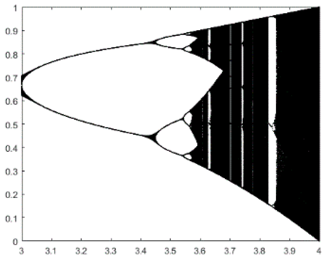
For instance, logistic chaos is widely used because of its simple expression and good performance, and it is shown in Figure 2. As can be seen, the logistic system has missed certain values. In consideration of the multilevel color image segmentation problem, this paper proposes a new chaotic map as follows:
where is the random value between 0 and 1.
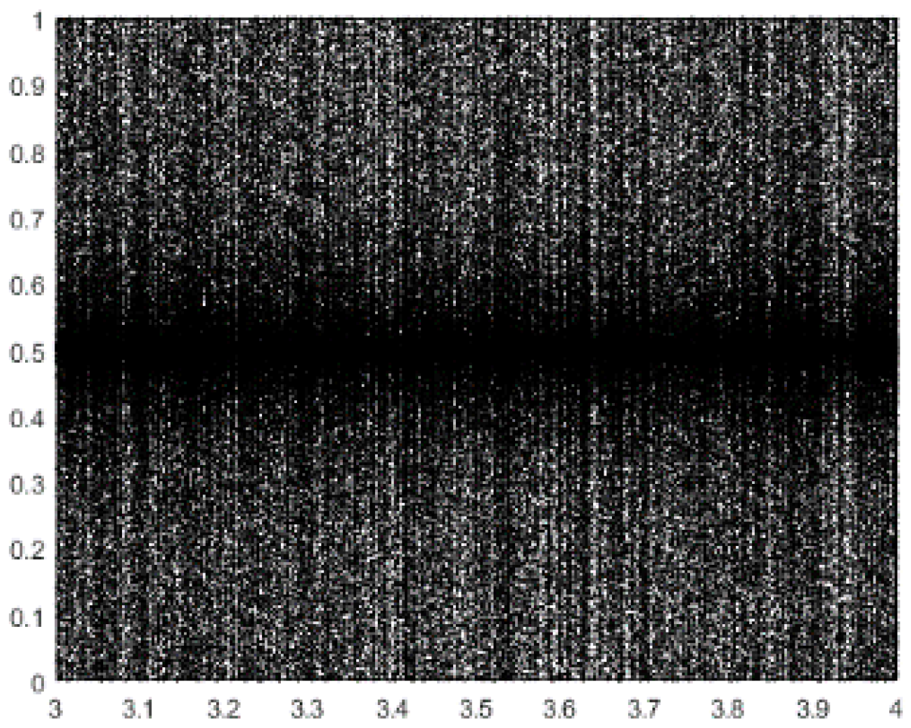
The new chaotic map is shown in Figure 3 and its distribution is more symmetrical than Logistic chaotic map. Taking advantage of this chaos strategy in EFO, the total performance of the algorithm will be improved and it is known as CEFO. The pseudo-code of the CEFO algorithm is presented in Algorithm 1.
| Algorithm 1. Pseudo-code of CEFO algorithm |
| /* Part 1: Algorithm parameters initialization */ |
| : The number of electromagnets in each electromagnetic particle. |
| : The number of electromagnetic particles in population. |
| : The probability of changing one electromagnet with a random electromagnet. |
| : The probability of selecting electromagnets from the positive field. |
| : The portion of particles belonging to positive. |
| : The portion of particles belonging to negative. |
| min = lower boundary; max = upper boundary |
| /* Part 2: Main loop of the algorithm */ |
| for i = 1 to do |
| for j = 1 to do |
| position [i, j] = min + rand ( )(max − min) |
| end for |
| end for |
| Update position by using the chaotic map of Equation (5) |
| fitness = function (position) |
| while t (current iteration) < max iterations |
| Divide the electromagnetic field into three regions |
| for i = 1 to do |
| if rand (0,1) > |
| Generate the by Equation (4) |
| else |
| Generate the from positive particles |
| end if |
| Check if any particle beyond the search space |
| end for |
| if rand (0,1) < |
| Change one electromagnet of randomly |
| end if |
| Compare the fitness of with worst particle |
| t = t + 1 |
| end while |
| Output the best particle |
4. Thresholding Segmentation Methods
The process of multilevel thresholding color image segmentation is to find more than two optimal thresholds to segment three components (red, green, and blue) respectively. In RGB images, each color component consists of pixels and number of gray levels. The obtained thresholds are within the range of [0, ], is considered as 256 and each gray-level is associated with the histogram representing the frequency of its gray level pixel used by .
4.1. Between-Class Variance Thresholding
Between-class variance (Otsu’s) [5] thresholding method can be defined as follows:
Assuming that thresholds form the threshold vector to split an image into n classes:
Constructing image histogram , where is the frequency of gray-level . Then, the probability of gray-level can be represented as:
For every class , the cumulative probability and average gray level in every region can be defined as:
and Otsu’s function can be expressed as:
where is the average gray intensity of the image.
Therefore, the optimal threshold vector is as follows:
4.2. Kapur’s Entropy Thresholding
Kapur’s entropy method maximizes the entropy value of the segmented histogram such that each separated region has more centralized distribution [39]. Extending Kapur’s entropy for multilevel image segmentation problem:
where represents the entropy value of j-th region in the image.
There are thresholds which can be configured as the dimensional optimization problem. And the optimal threshold vector is obtained analogously by:
4.3. Fuzzy Entropy Thresholding
In the fuzzy entropy technique, let an original image be , where and represent the width and height of an image. Supposed that and are two thresholds to divide the original image into 3 parts named as , , [10]. consists of pixels of low gray levels; is made of pixels with middle gray levels; is composed of pixels of high gray levels. Usually, using (13) to calculate the image histogram:
where ; is the number of the k-th pixel in ; is the histogram of the image at gray-level , .
Consider as an unknown probabilistic partition of , whose probability distribution can be expressed as:
For each , let:
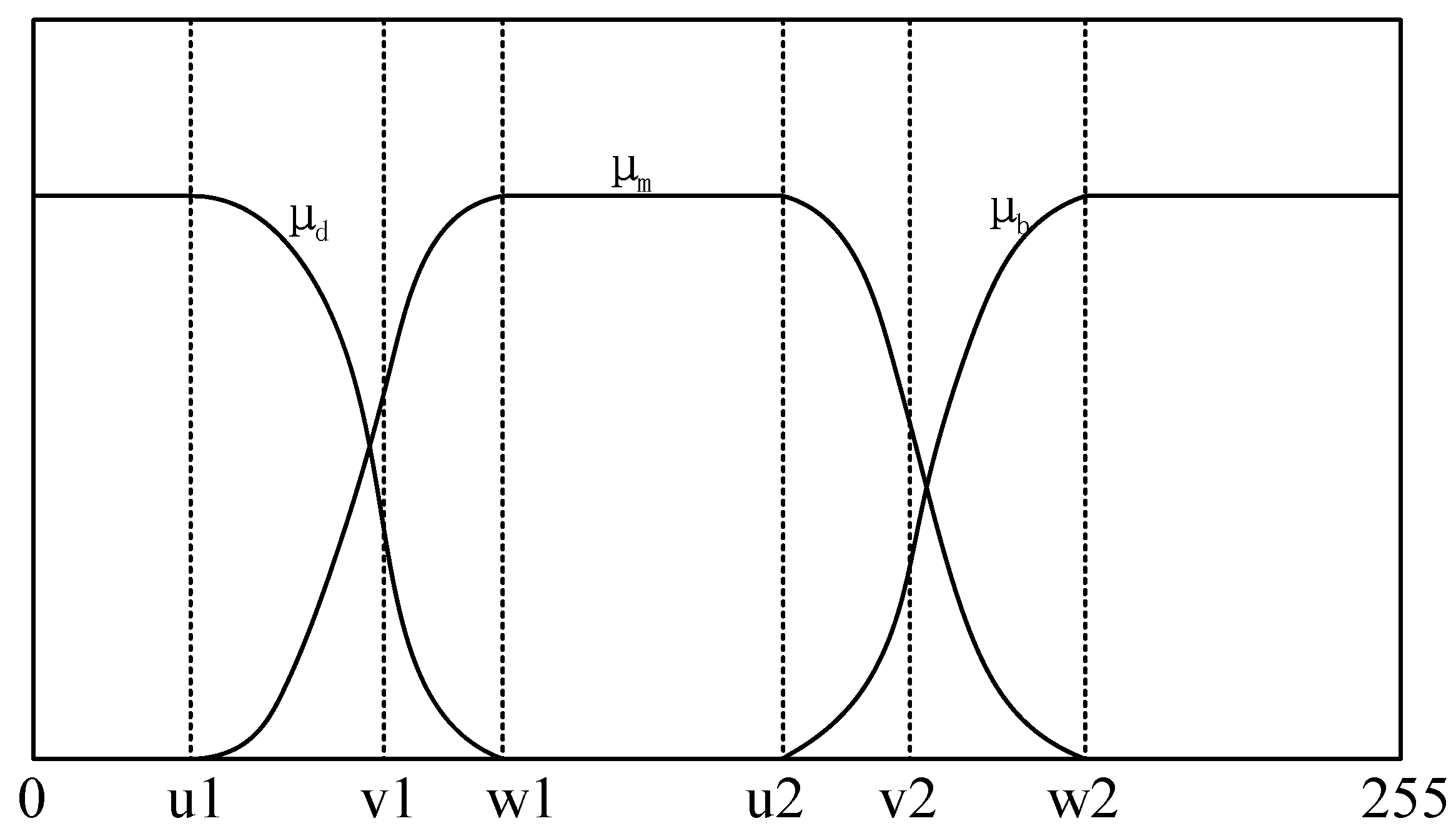
Utilizing , , as the membership functions of , , , which is shown in Figure 4 [40]. There are six fuzzy parameters of , , , , , in the membership functions, in other words, and are determined by these six parameters. According to the above statement, we can have the probability distribution of three regions expressed as:
where , , are the conditional probability of a pixel partitioned into three classes. Moreover, a pixel of in an image satisfies the constraint of .
The three membership functions have been shown in Figure 4. And these mathematical formulas are defined as follows:
where , , , , , should meet the condition of .
Then, the fuzzy entropy of each part is as follows:
The whole fuzzy entropy function is defined as:
Equation (21) is determined by six variables which are called fuzzy parameters. Seeking the optimal group of , , , , , when (21) reach the maximum value. Therefore, the most applicable threshold can be calculated as:
As is shown in Figure 4, according to the above equation, and can be defined by (17)–(19), and the result is as follows:
Fuzzy entropy thresholding can meet the requirement from single threshold segmentation to multiple thresholds segmentation, and the optimal threshold vector obtained is more precise. However, each threshold should be determined by three parameters in fuzzy entropy thresholding, and thresholds need to be defined by 3n fuzzy parameters [41,42].
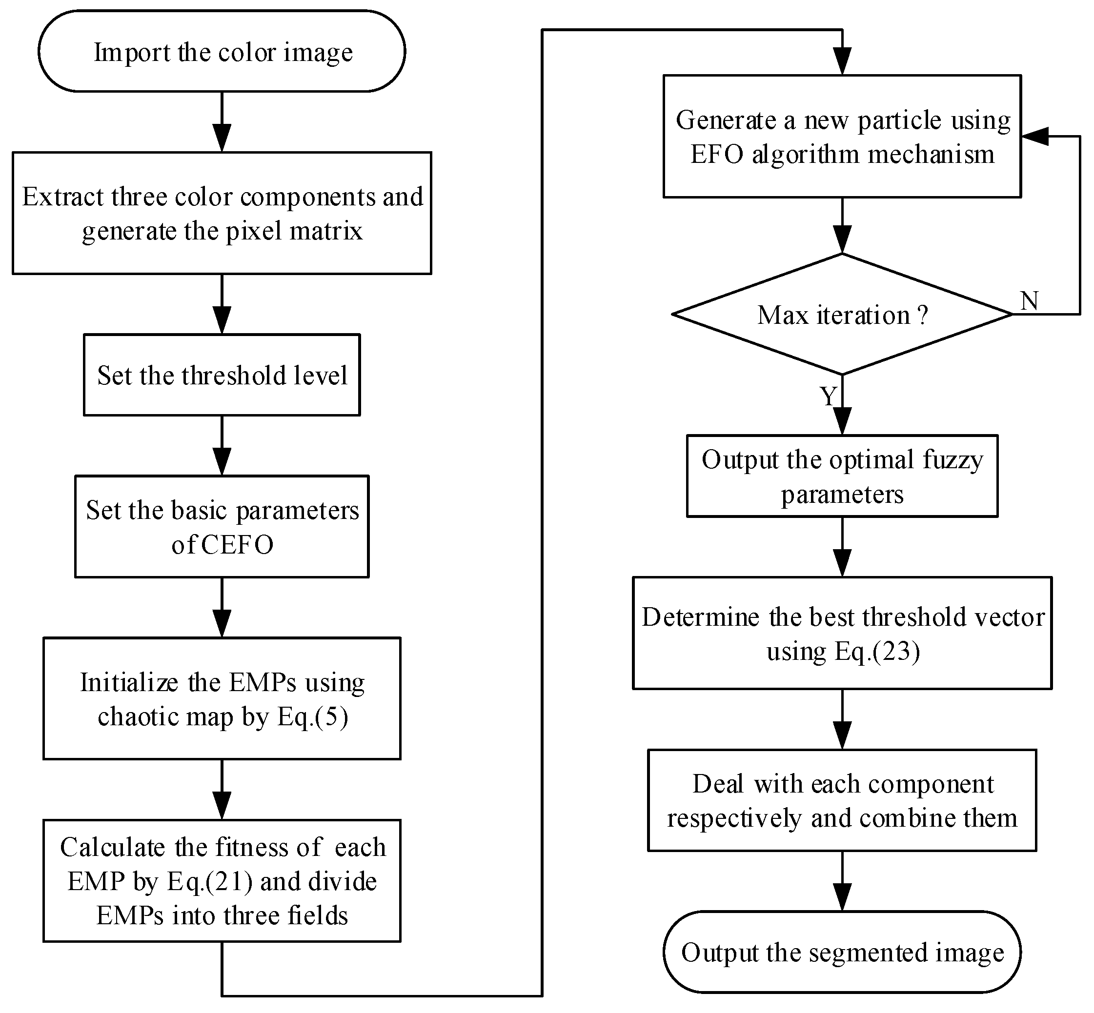
With the increase of threshold level gradually, the degree of the computation will be significantly risen, which diminish the speed of the process and the practicability will be reduced. In order to improve the convergence efficiency, it is necessary to use the optimization algorithm for searching the optimal threshold vector. This paper takes advantage of the CEFO to ensure the segmentation accuracy and greatly decrease the execution time. The general flow of fuzzy entropy thresholding based on the CEFO algorithm is presented in Figure 5.
5. Experimental Environment
In order to verify the superiority of the CEFO algorithm in dealing with the multilevel color image segmentation problem, this section will introduce the description of our benchmark images and then select several other algorithms for comparison. The parameters of each algorithm will be described firstly and a series of quality metrics used to evaluate the quality of segmented images will be calculated at the end.
5.1. Benchmark Images
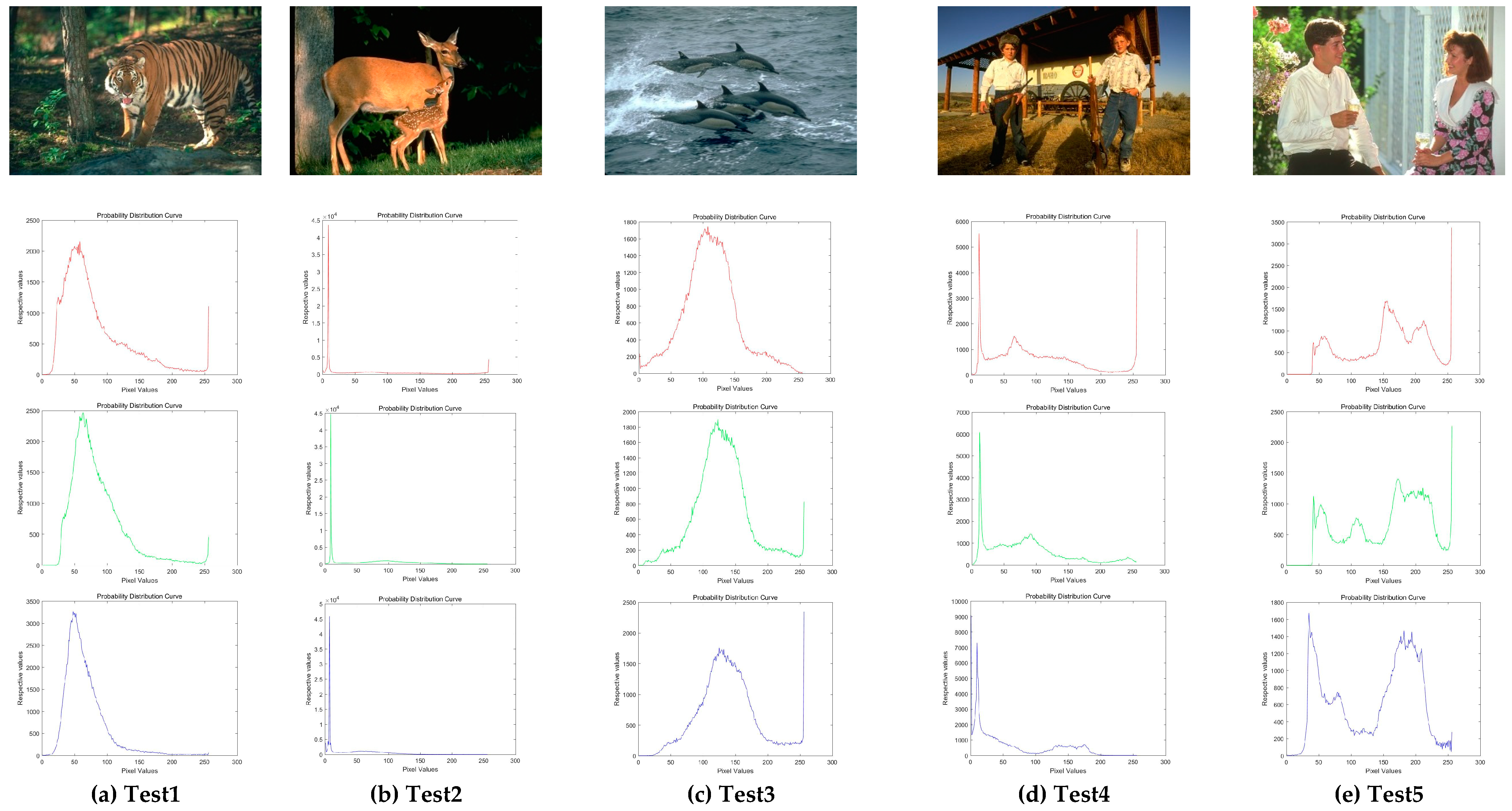
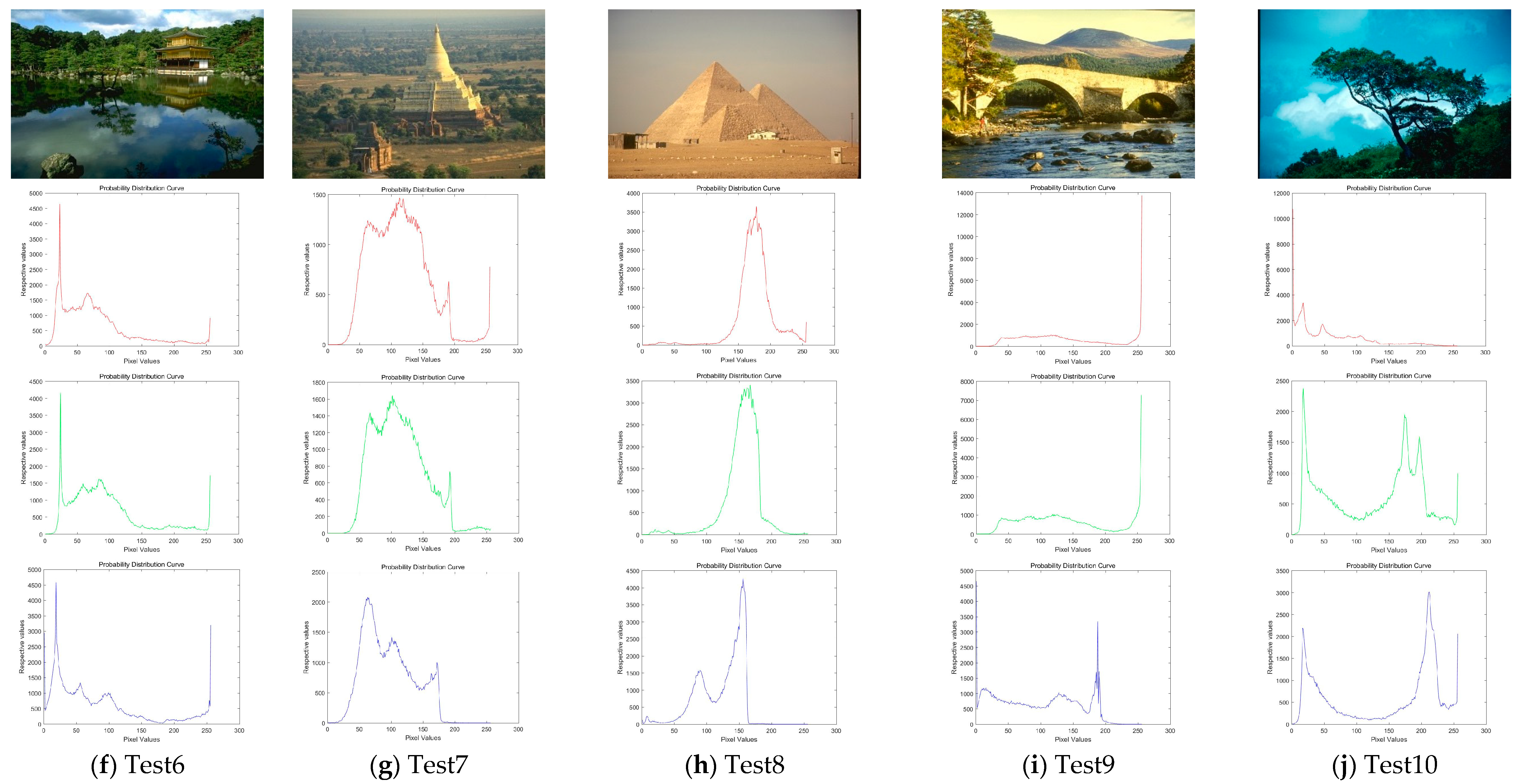
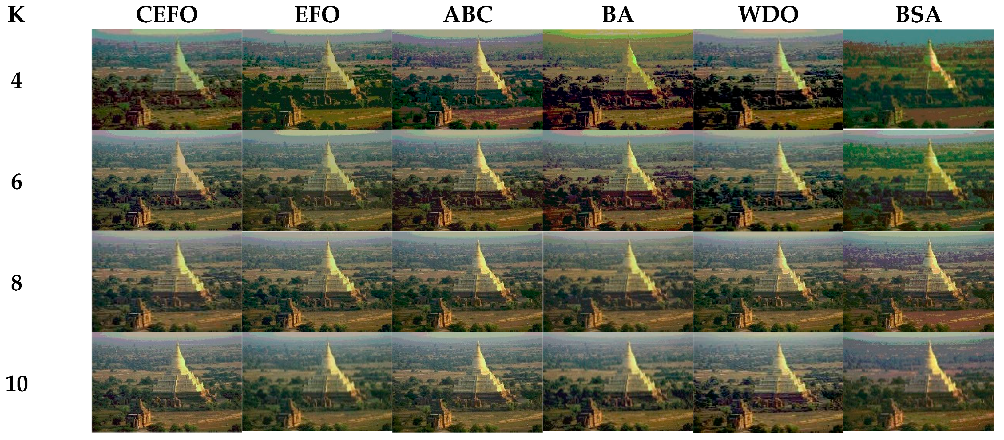
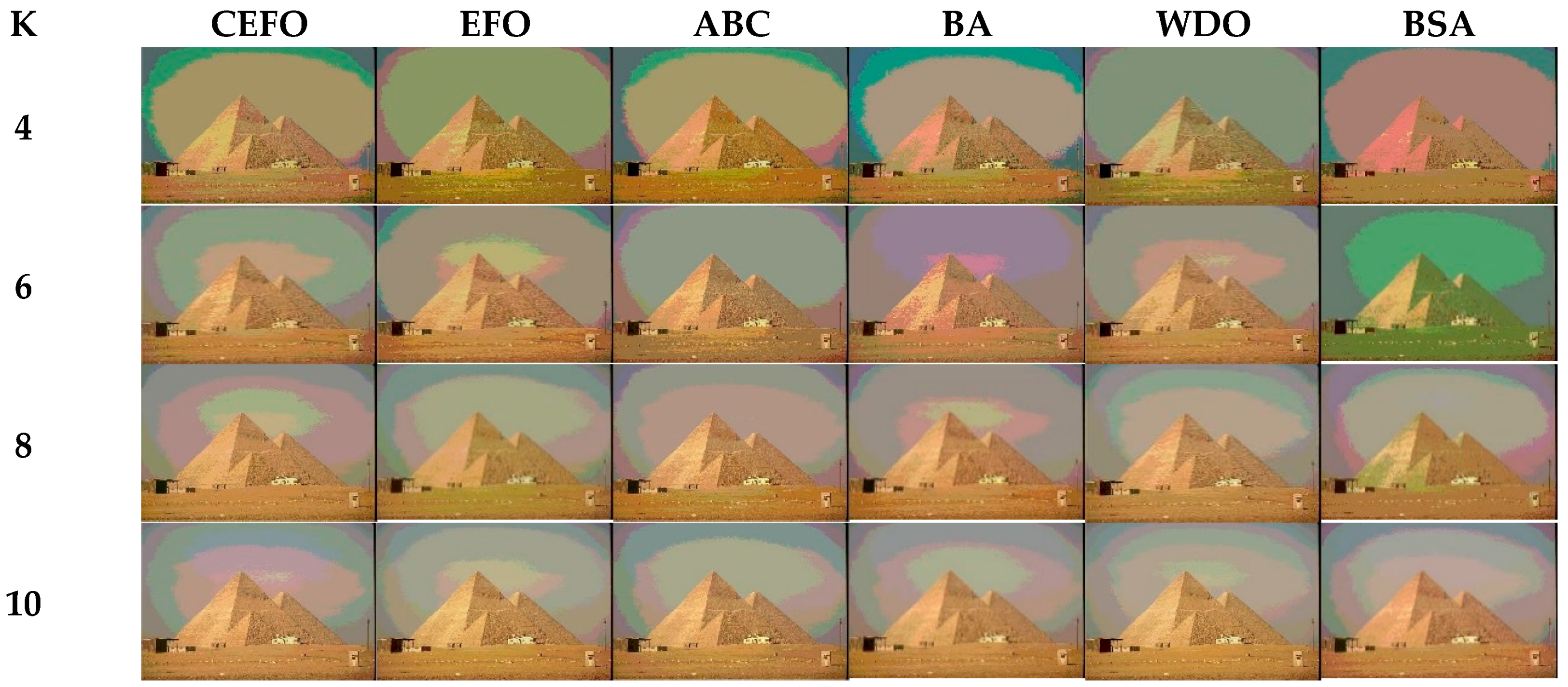
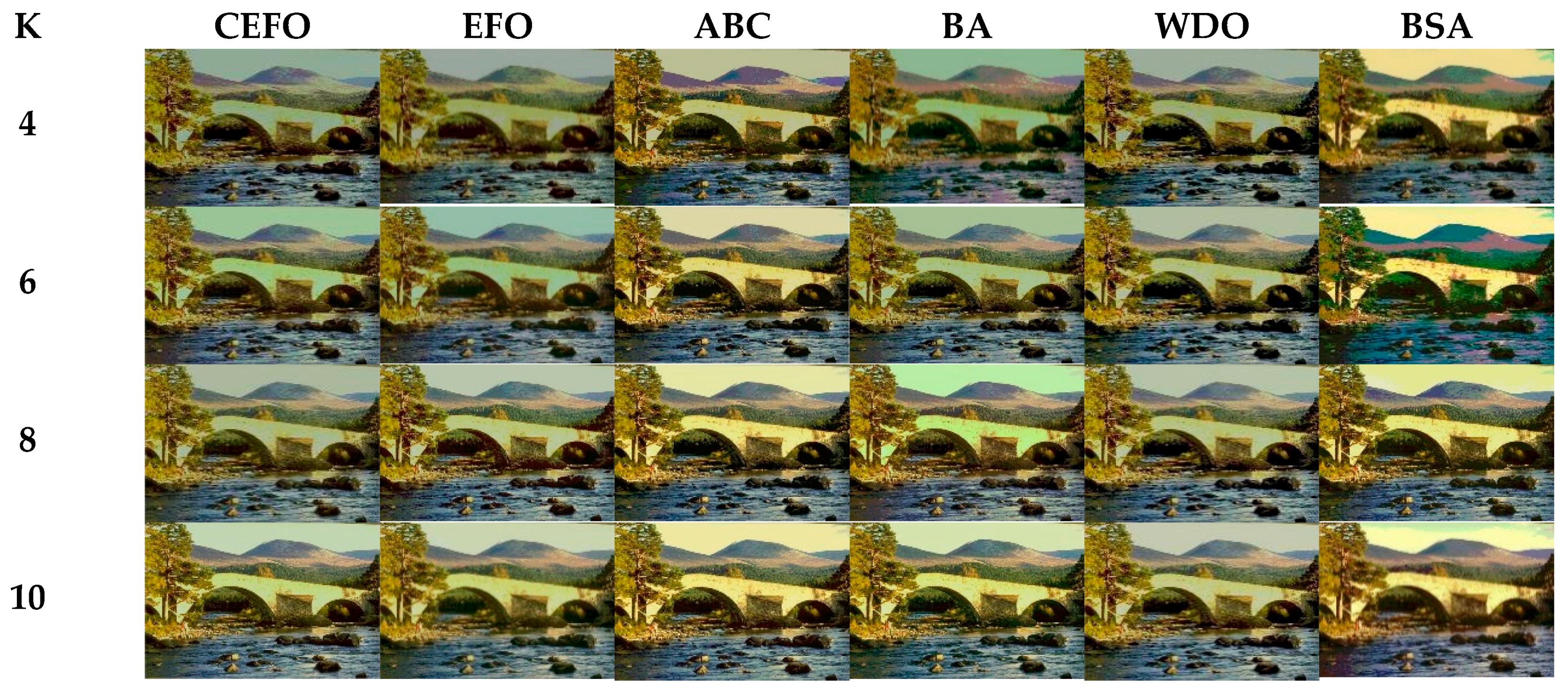
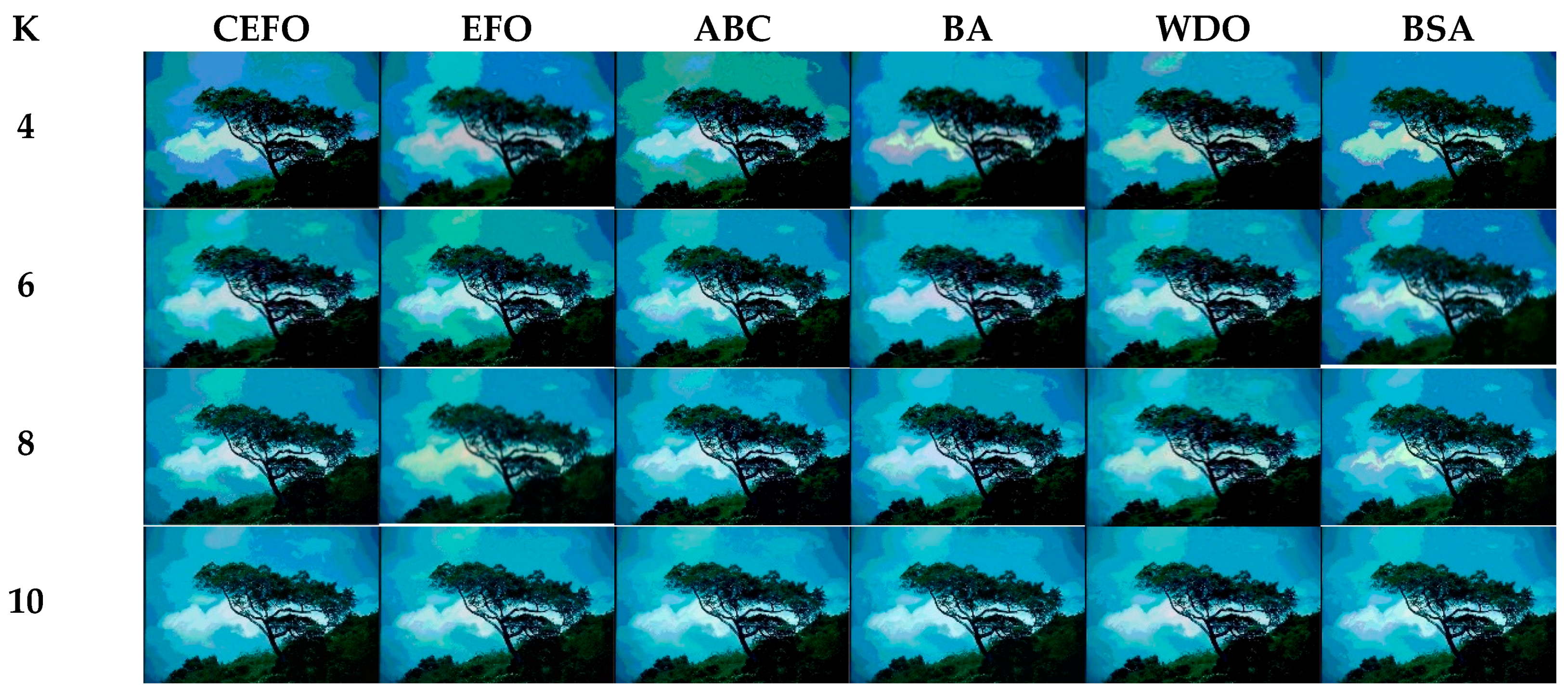
In this experiment, ten images are chosen from the Berkeley segmentation data set, which is shown in Figure 6. It has presented the histogram of three components about every color image. Among these images, Test 1–3 are animal images; Test 4 and 5 are about human; Test 7 and 8 are landmark buildings; Test 6 and 9 are images related to landscape architecture; Test 10 is the normal scenery image.
5.2. Experimental Settings
When applied to solve the problem of multilevel color image segmentation, different meta-heuristic algorithms have different optimization performances due to their strategies and mathematical formulations [43]. Therefore, it is essential to compare the CEFO algorithm with other different algorithms such as EFO, ABC [44], BA [10], BSA [19], WDO [23]. Among these algorithms, ABC, BA, and BSA are proposed from biology; EFO and WDO are inspired from physics. The number of maximum iterations of each algorithm is set to 500, and the initial population is set to 15, with a total of 30 runs per algorithm, other specific parameters are presented in Table 2.
All the algorithms are programmed in Matlab R2016a (The Mathworks Inc., Natick, MA, USA) and implemented on a Windows 7 – 64 bit with 8 GB RAM environment.
5.3. Segmented Image Quality Metrics
To evaluate the quality of segmented images under different algorithms at selected threshold levels, four metrics are selected as follows [45,46]:
- Peak Signal to Noise Ratio (PSNR)
The index is used to measure the difference between the original image and the segmented image, and a higher value is gained when the segmented image has a better effect. It can be defined as:
where and represent the size of the image; is the original image; is the segmented image.
- Mean Structural Similarity (MSSIM)
The index evaluates the overall image quality, which is in the range of . The higher value of MSSIM is obtained when it represents the segmented image is more similar to the original image. The MSSIM is the average of every component and SSIM can be calculated as:
- Feature similarity (FSIM)
The index is in the range of , and the segmented image is better when the value is closer to 1. The FSIM can be expressed as:
- Computation Time (CPU Time)
The index measures the convergence rate of each algorithm. The algorithm is more efficient when the time is shorter.
6. Results and Discussions
6.1. Comparison of Other Meta-Heuristic Algorithms
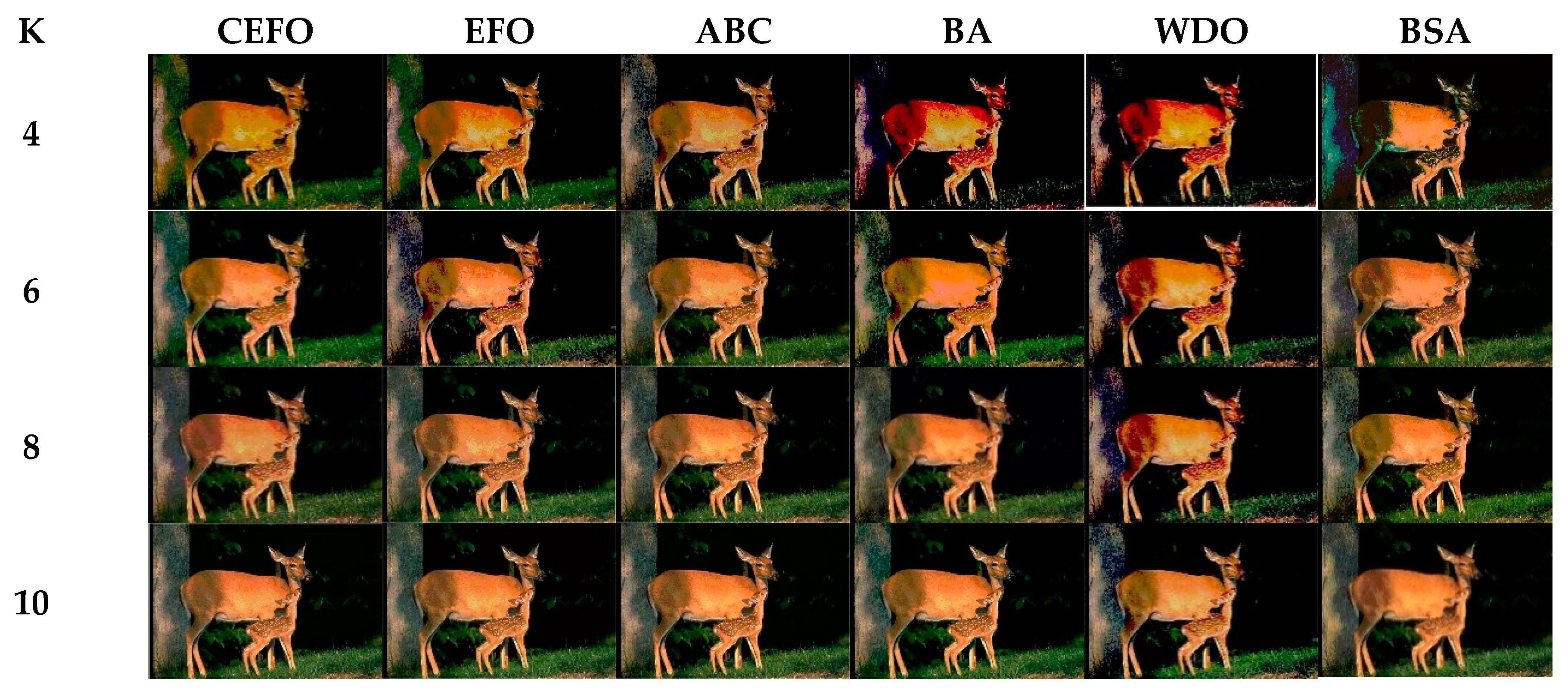
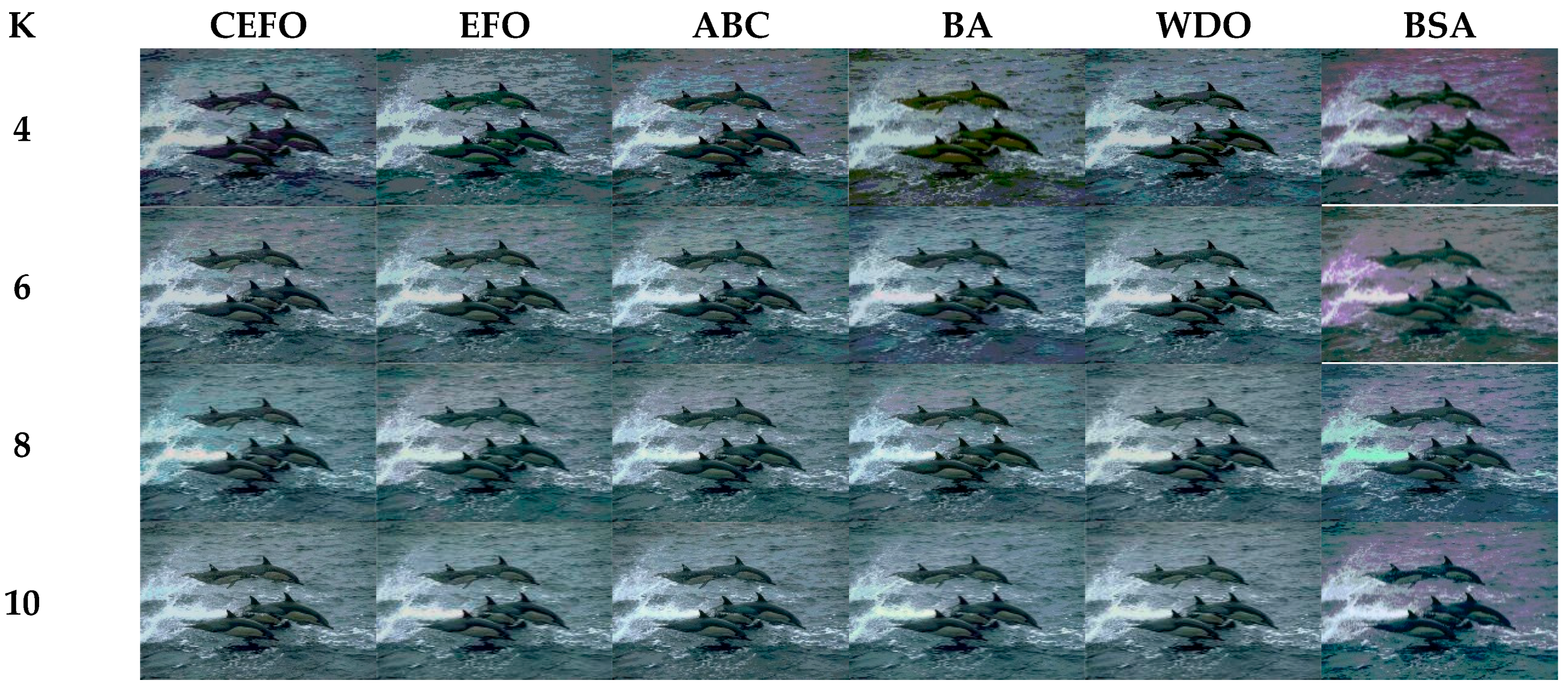
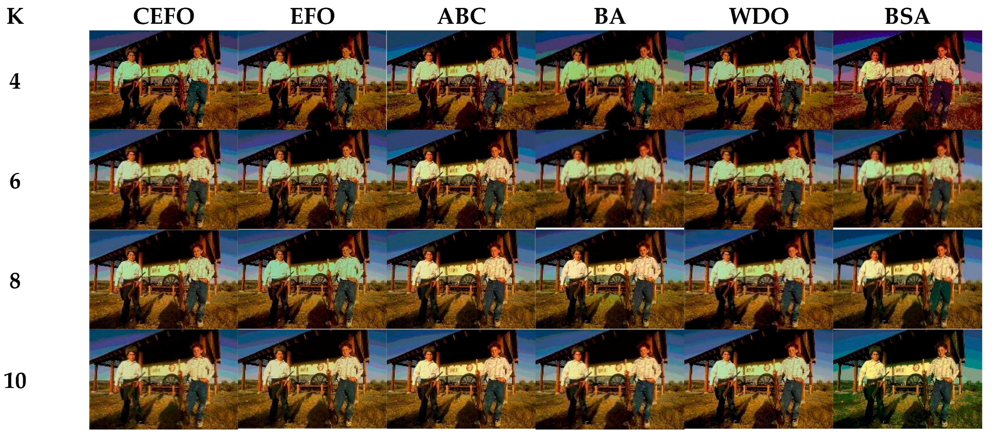
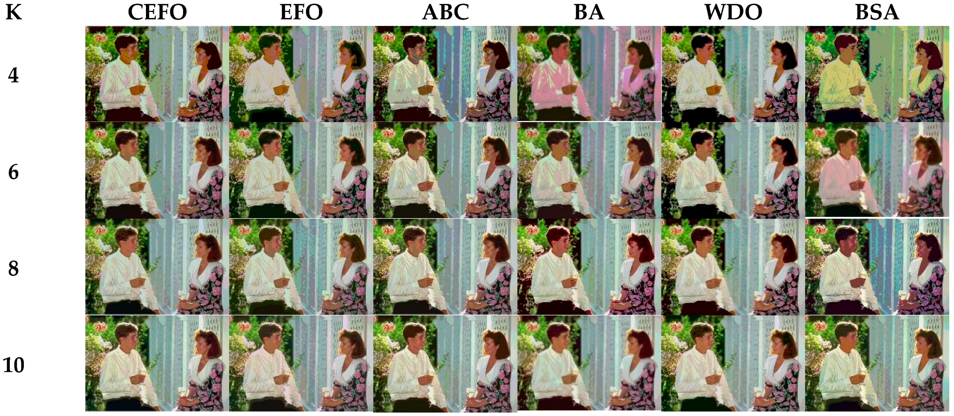
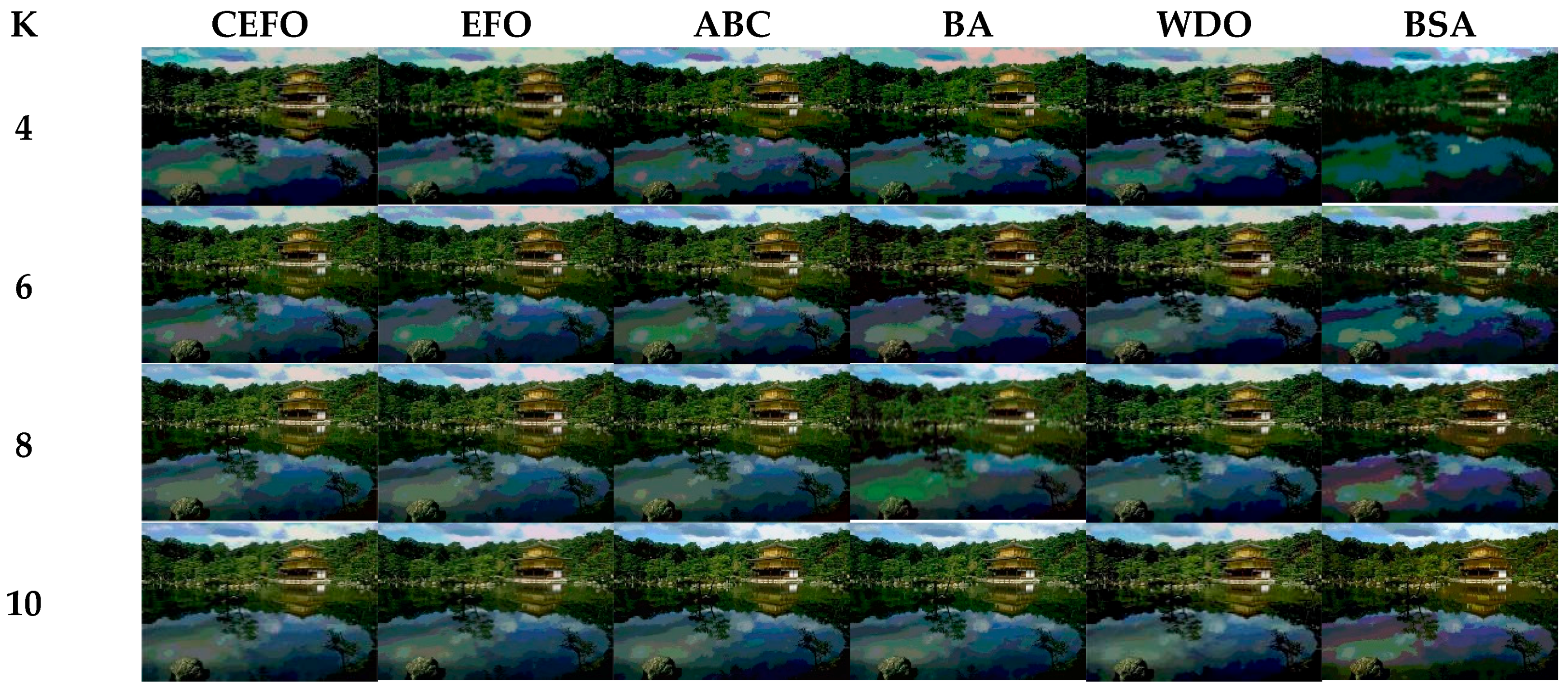
Utilizing 6 algorithms based on fuzzy entropy criterion to conduct the experiment on 10 images at the threshold level of 4, 6, 8, and 10 ( = 4, 6, 8, 10). The results of the optimal threshold vector are presented in Table 3, Table 4 and Table 5 exhibiting each threshold level of three component about every image. And the results of segmented images are presented in Figure 7, Figure 8, Figure 9, Figure 10, Figure 11, Figure 12, Figure 13, Figure 14, Figure 15 and Figure 16, which take each Test image as a group. Furthermore, the results of the four metrics are shown in Table 6 and Table 7.
Table 6 and Figure 17 and Figure 18 compare the CPU Time and PSNR values while Table 7 and Figure 19 and Figure 20 compare the MSSIM and FSIM values of the segmented images. As can be seen from these tabulated values, all algorithms have lower values of PSNR, MSSIM, and FSIM at lower threshold levels. With the improvement of the threshold level, the values of PSNR, MSSIM, and FSIM increase gradually. Consequently, it can be clearly known that segmentation performance will be improved as the threshold level increases. However, the time of each algorithm will rise equally on the increasing threshold levels indicating the computation of algorithms is more complex on the higher threshold levels. PSNR, MSSIM, and FSIM are used to measure the similarity and qualify among the segmented images. Higher PSNR, MSSIM, and FSIM demonstrate that segmented images have more excellent segmentation performances.
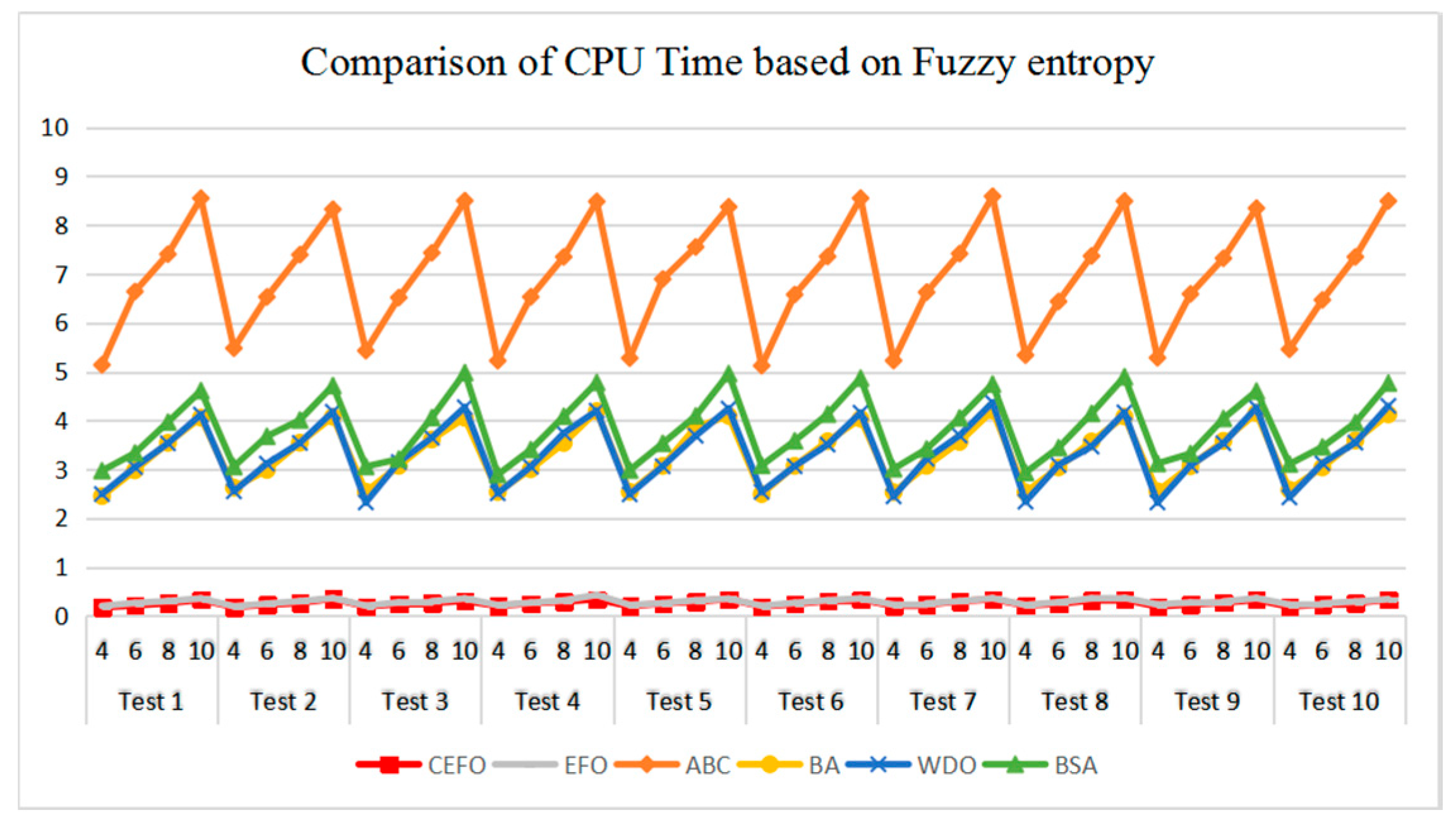
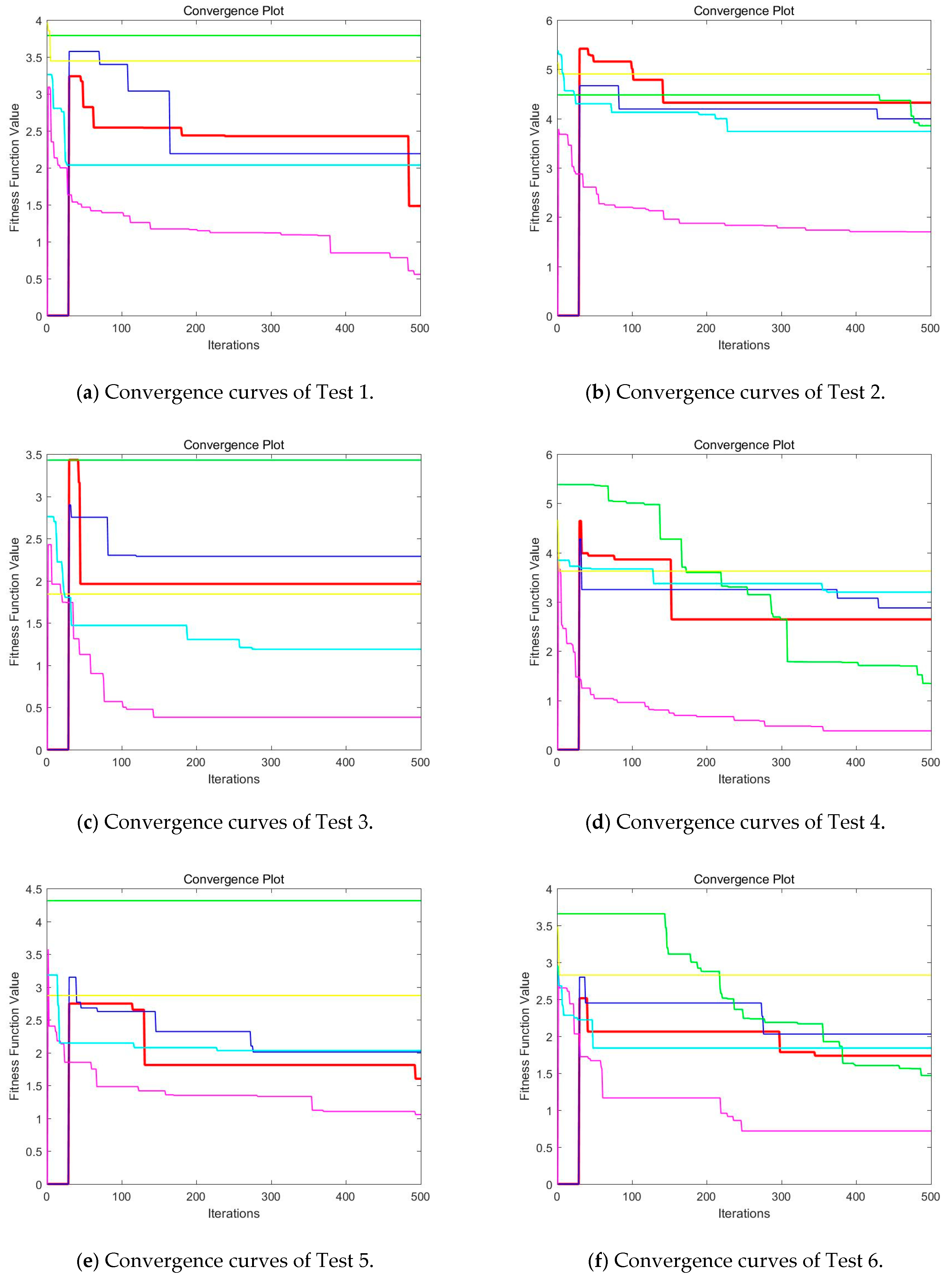
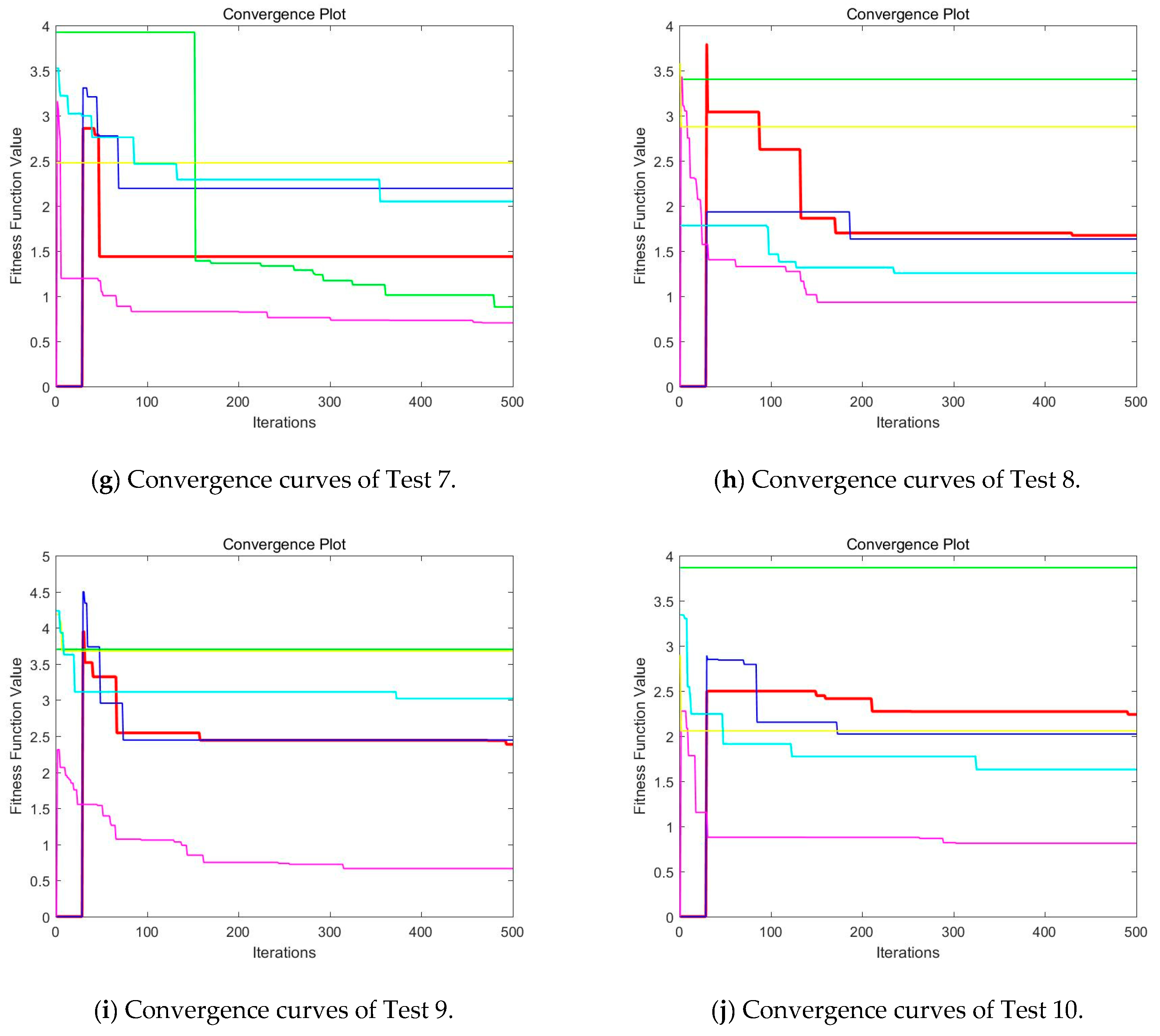
Then, when comparing the differences in CPU time between various algorithms, it can be found that CEFO and EFO are significantly faster than ABC, BA, WDO, and BSA. Moreover, the running time of CEFO has decreased about 12.26% when comparing with EFO, which indicates the modified electromagnetic field optimization algorithm has a faster convergence rate. As for other algorithms, ABC has the longest time of computation due to its slow convergence rate, it needs nearly 30 times as much as CEFO. Afterward, BA, WDO, and BSA have an approximate running time, they are about 15 times longer than CEFO. With the increase of execution time, the practicability of the algorithm will be reduced. For a clearer presentation of convergence speed about these algorithms, the convergence curves are shown in Figure 21.
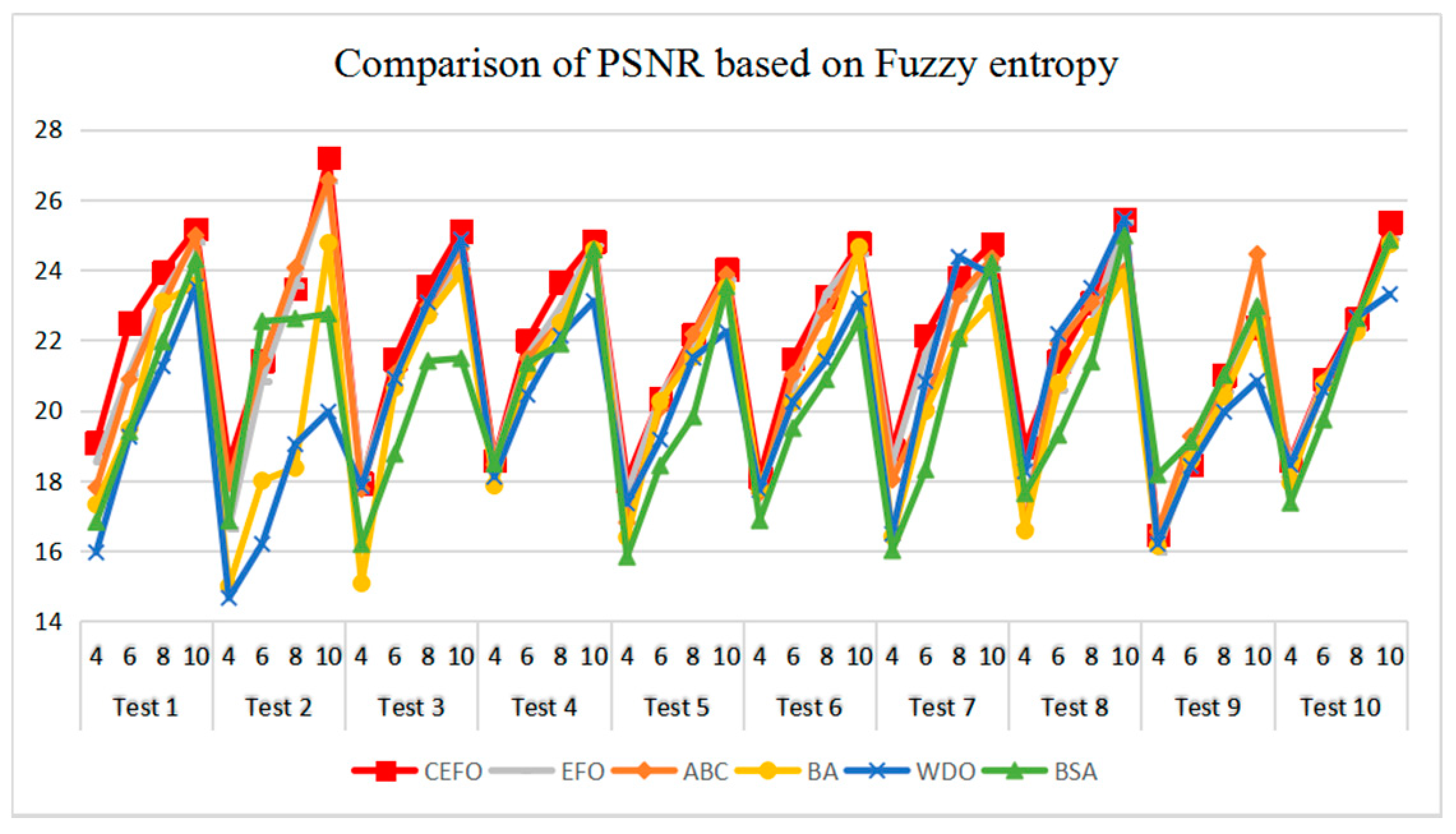
In terms of PSNR, the chart of all algorithms is shown in Figure 18. It can be seen that CEFO has higher values among these algorithms; ABC has similar values to EFO in some images at a high threshold level. For instance, in Test 1 of K=10, PSNR value of EFO is 24.8085 while ABC is 24.9762, but CEFO is 25.1603. WDO has much lower values in smaller threshold level and BSA has good values in higher threshold level, all in all, PSNR values of BA, WDO, and BSA have different diversification, but they are mediocre on the whole.
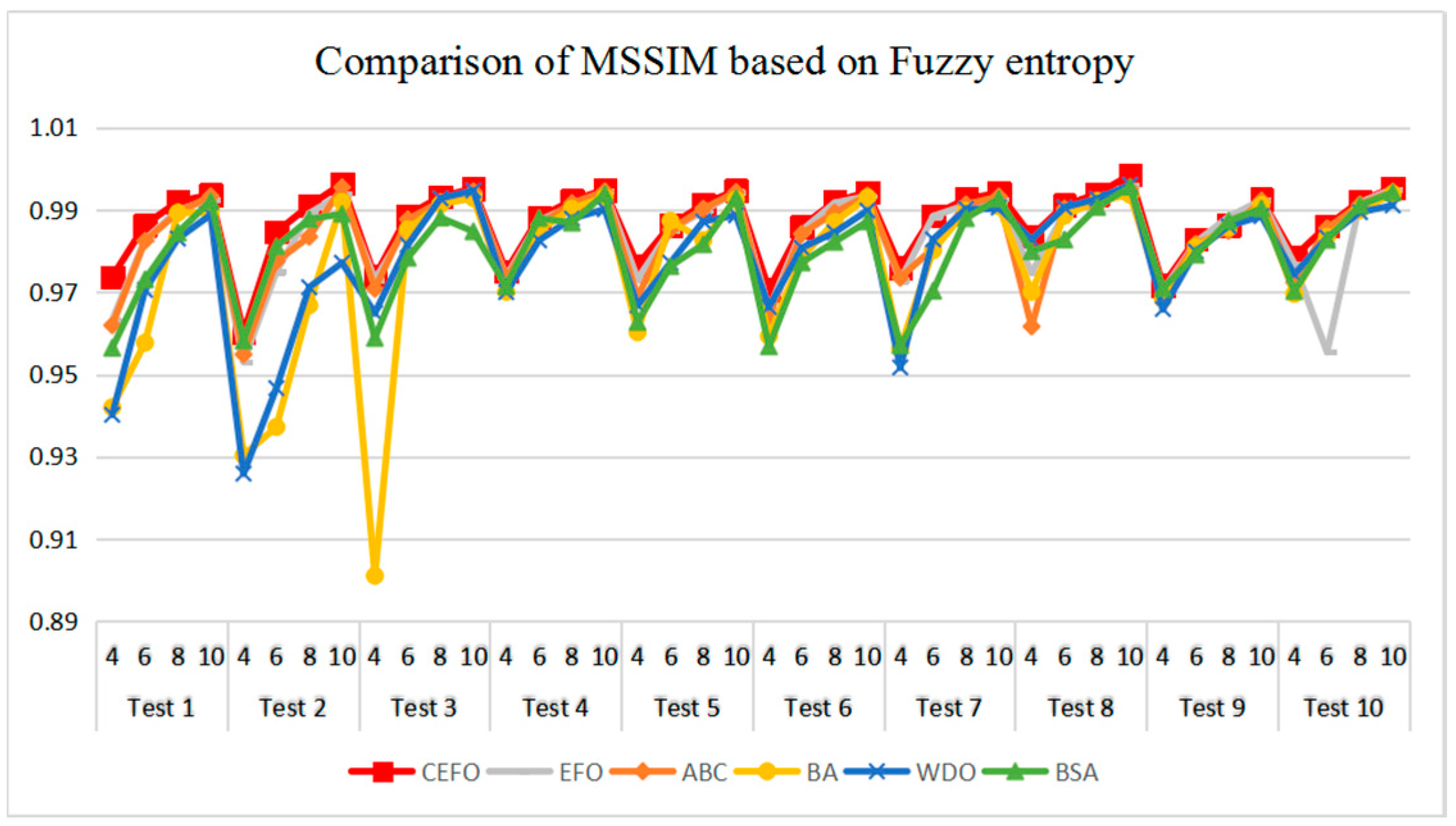
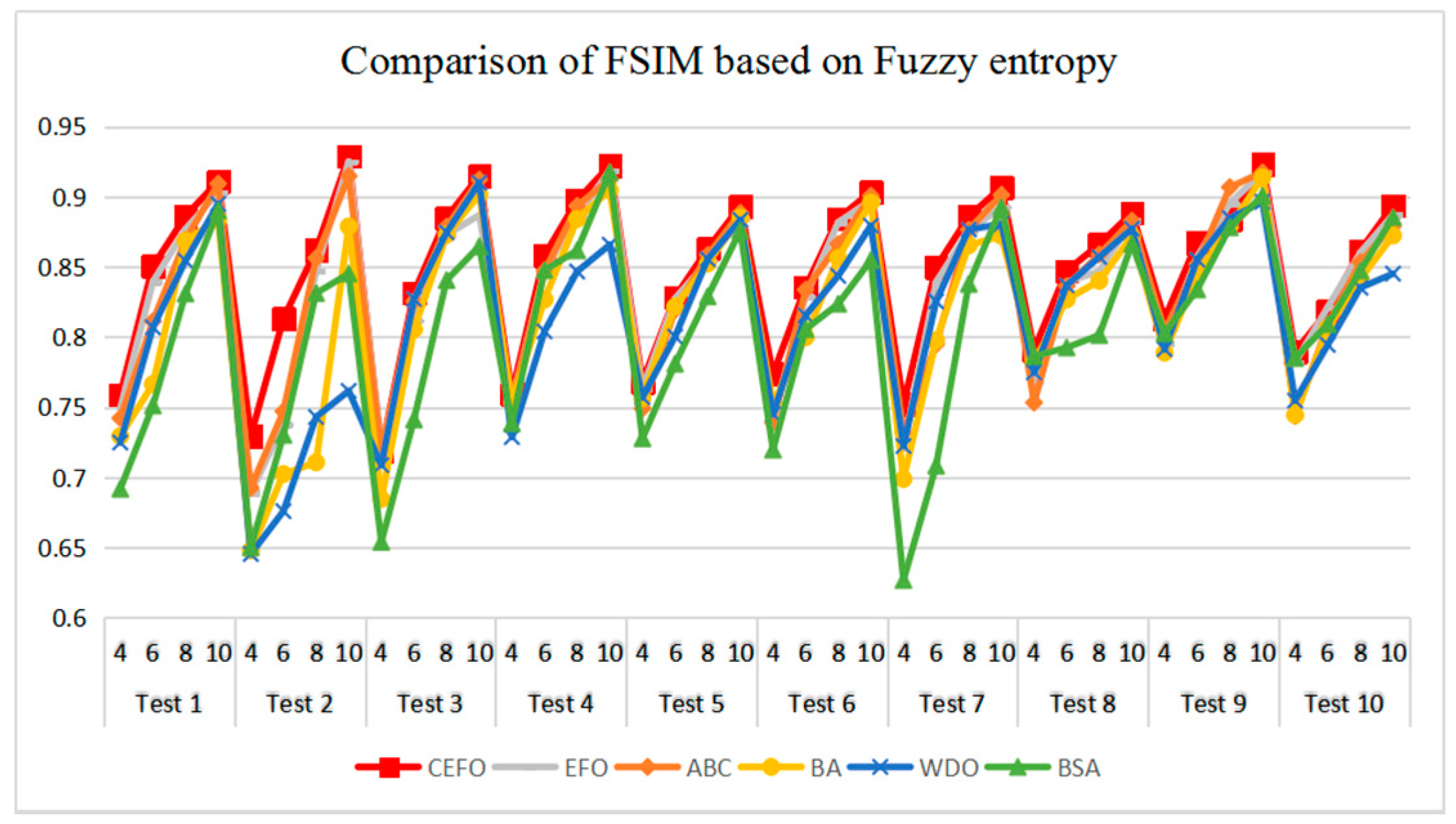
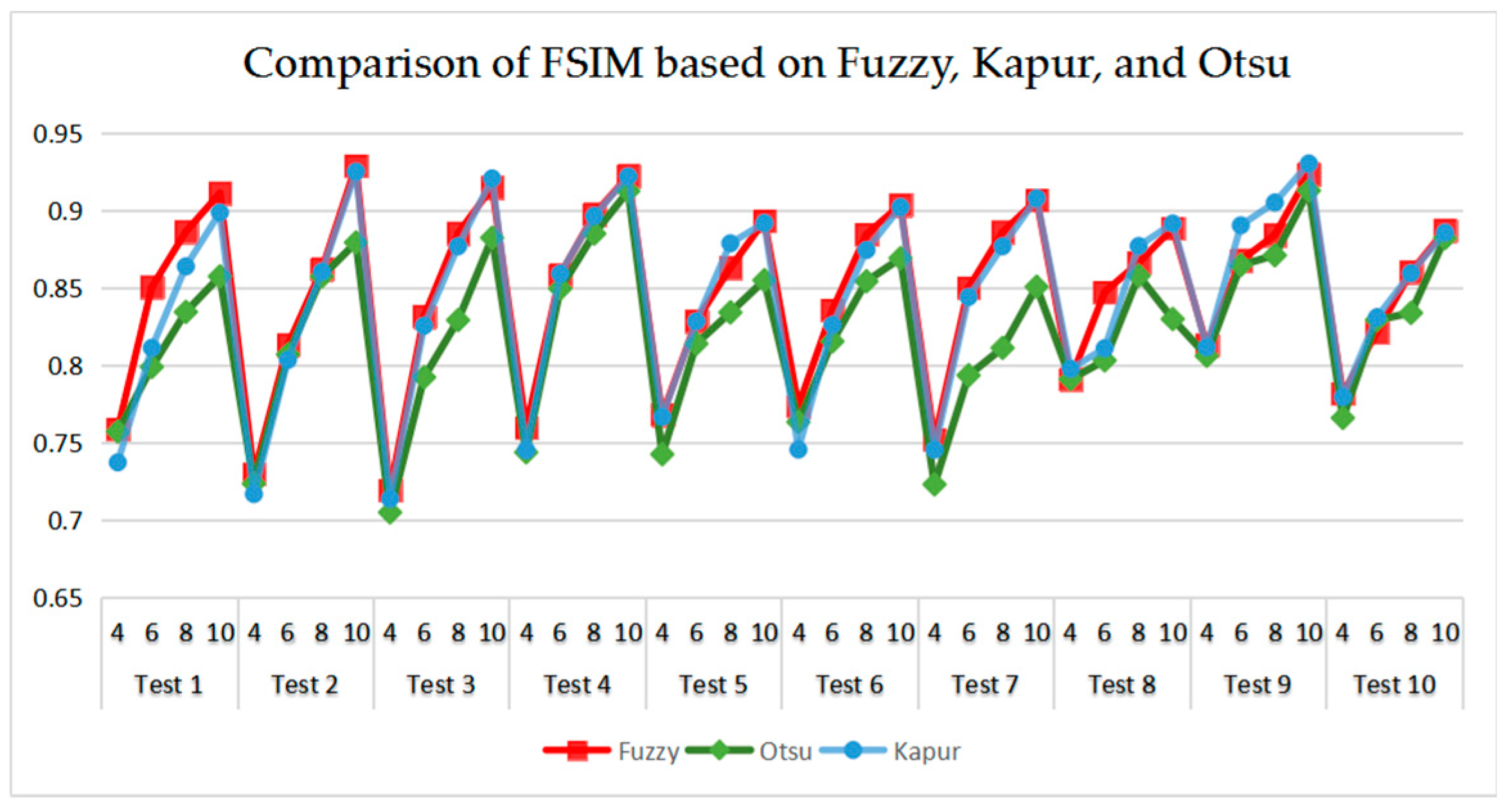
Comparing the results of MSSIM and FSIM in Table 7, FSIM is considered to be more authoritative and application and CEFO also performs better than other algorithms in this index. Although EFO can have a banner performance at K = 4, ABC will usually be close to EFO at high levels. BA has better values at some images such as in Test 2, 4, etc. WDO and BSA have higher values than BA at K = 6 in some images but they are all lower than CEFO on the whole.
From what has been mentioned above, the CEFO algorithm has superior performance when searching for the optimal threshold vector in multilevel thresholding color image segmentation.
6.2. Comparison of Other Segmentation Methods
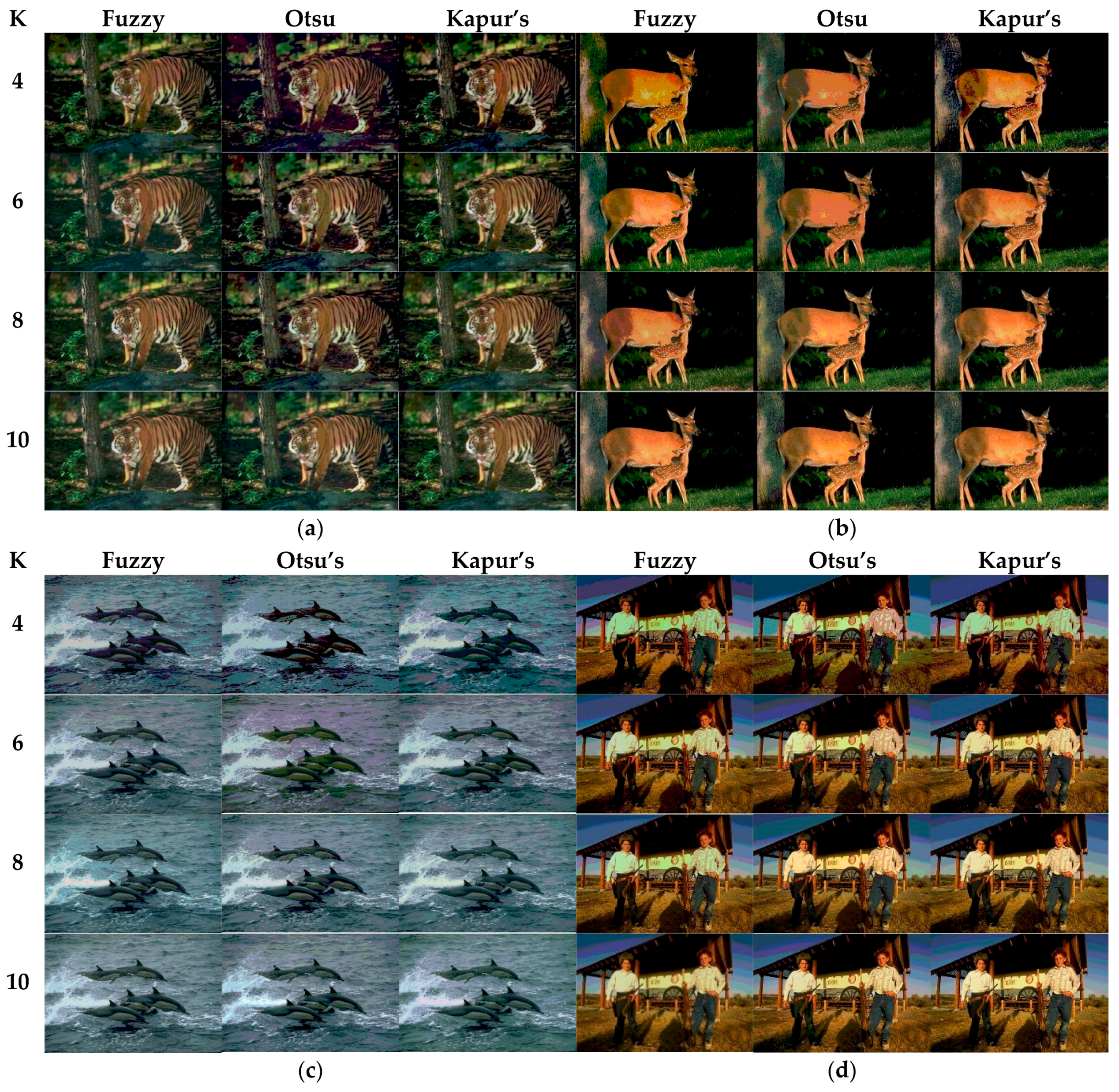
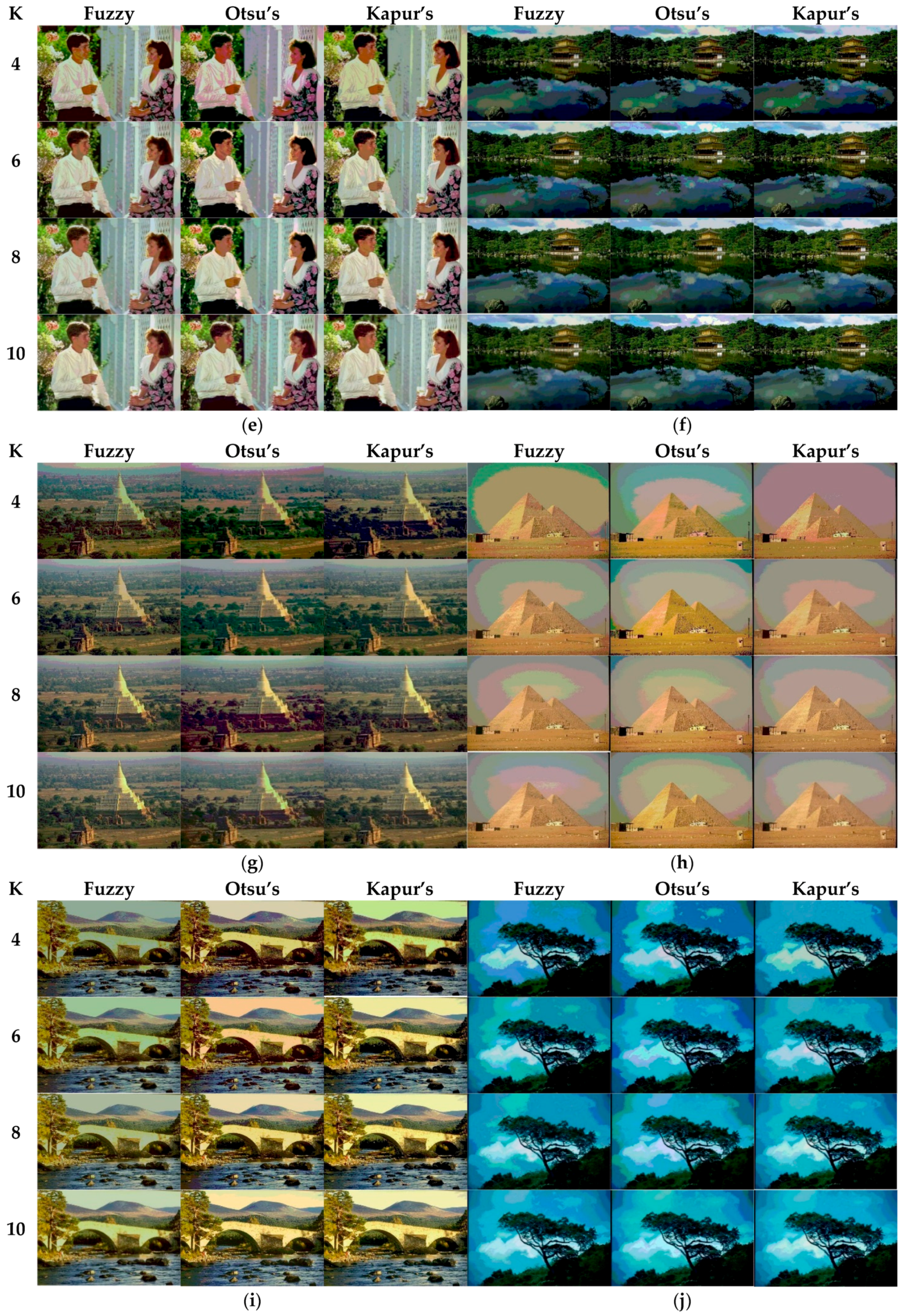
In the last experiment, the superiority of CEFO has been verified. And in this experiment, fuzzy entropy has been regarded as the research objective. To show the performance of fuzzy entropy thresholding in multilevel color image segmentation, Otsu’s and Kapur’s entropy based on color image segmentation are used to be a comparison. Applying the CEFO algorithm to Fuzzy entropy, Otsu’s, and Kapur’s entropy respectively to segment selected 10 Berkeley images in Figure 6. The threshold level is chosen as = 4, 6, 8, and 10, which is used to obtain the corresponding threshold points for each component of the color image. The results of segmented images are in Figure 22, and the corresponding optimal threshold values are in Table 8. Table 9 compares the performance of different thresholding approaches based on parameters of CPU Time, PSNR, MSSIM, and FSIM.
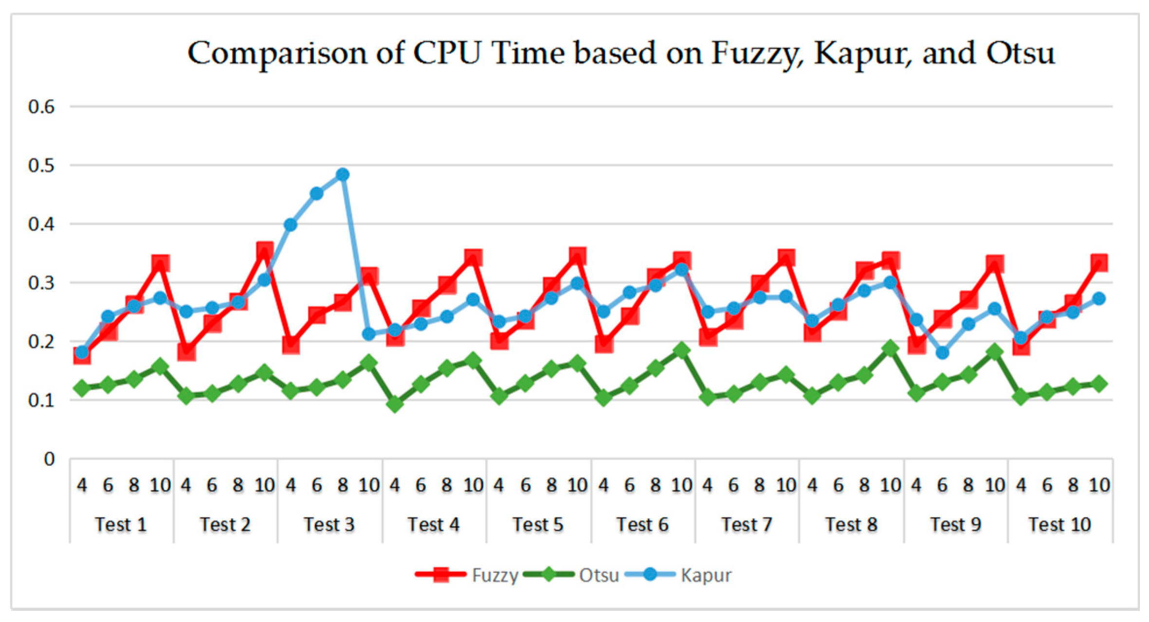
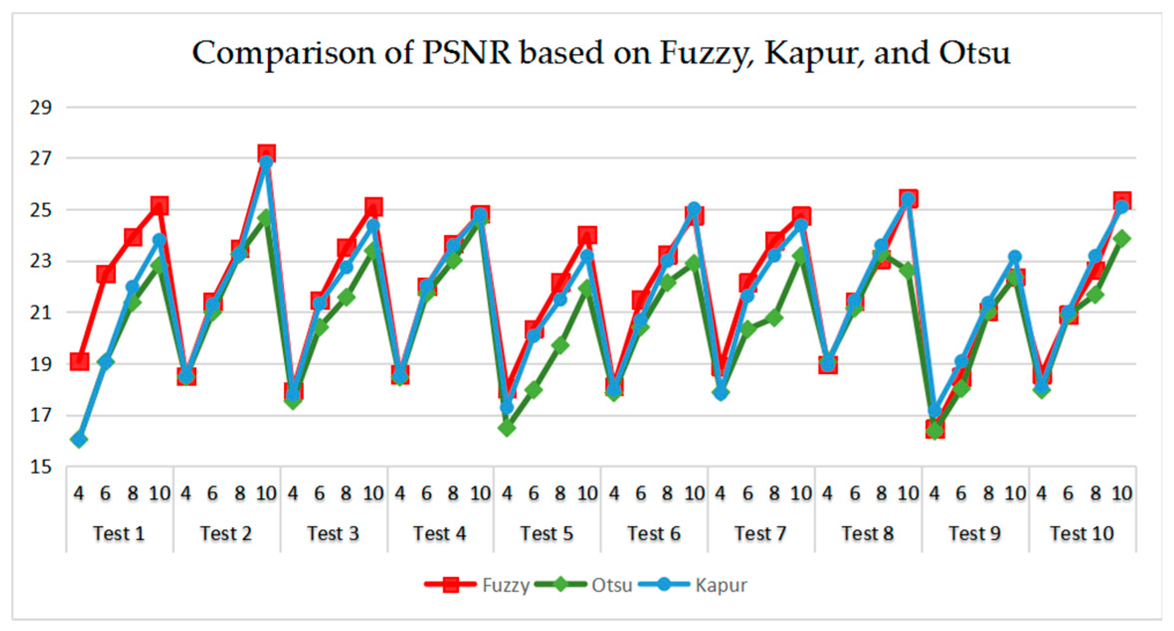
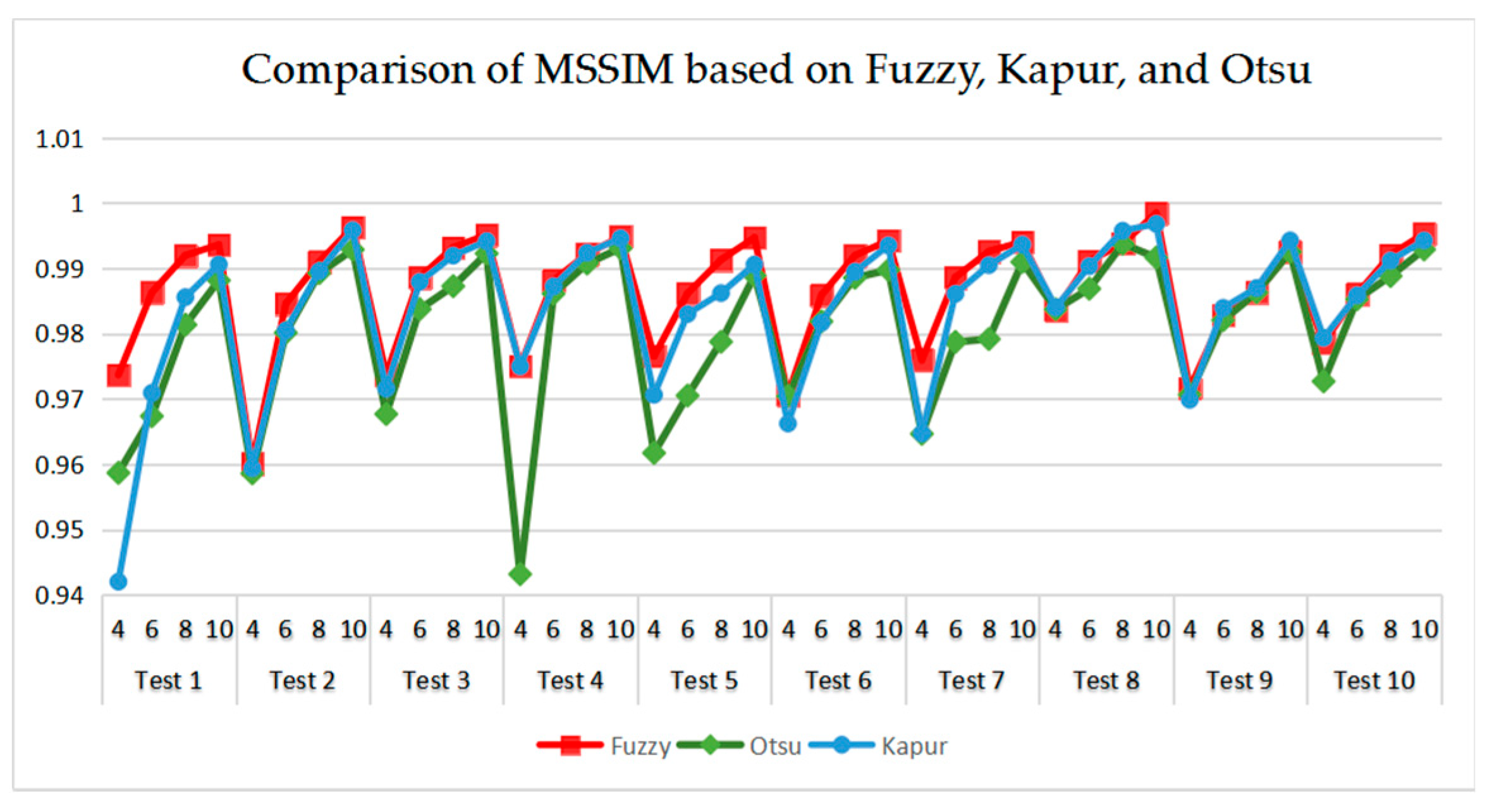
As can be seen in Table 9 and Figure 23, Figure 24, Figure 25 and Figure 26, Otsu’s thresholding has the fastest speed of execution time, fuzzy entropy and Kapur’s entropy are a bit slower than Otsu’s. However, three thresholding segmentation methods are all in 0.5 (seconds) at different threshold levels, which can also indicate CEFO algorithm has a fast convergence rate. In terms of PSNR, it is clear that fuzzy entropy thresholding has higher values in general, the ranking of PSNR among these segmentation methods is Fuzzy > Kapur’s > Otsu’s. As for MSSIM and FSIM, Fuzzy entropy also performs well, which is in advance of two other methods overall. And the ranking of MSSIM and FSIM among three methods is Fuzzy > Kapur’s > Otsu’s. Therefore, fuzzy entropy is better as compared to others showing CEFO based on the fuzzy entropy technique can be applied in the color image segmentation field excellently.
6.3. ANOVA Test
A statistical test known as “the analysis of variance” (ANOVA) has been performed at 5% significance level to evaluate the significant difference between algorithms. In the experiment, CEFO algorithm is regarded as the control group and is compared with EFO, ABC, BA, WDO and BSA algorithms in terms of four measure metrics. The null hypothesis assumes that there is no significant difference between the mean values of 5 selected algorithms, whereas, the alternative hypothesis can be considered as a significant difference between them. Table 10 exhibits the –value of CPU Time, PSNR, MSSIM, and FSIM by the ANOVA test. As can be seen, the -value for CPU Time is less than 0.05, which implies a significant difference between the proposed algorithm and other algorithms and CEFO has a much fast convergence rate. With respect to another three measures, CEFO also has significant difference about BA, WDO and BSA. It can be observed that CEFO algorithm has a better performance.
7. Conclusions and Future Work
In this paper, multilevel thresholding color image segmentation has been considered as an optimization problem in which the fuzzy entropy technique has been presented as the objective function. To achieve efficient segmentation, it is essential for algorithms to search the optimal fuzzy parameters and threshold values. Electromagnetic Field Optimization is a novel meta-heuristic algorithm which use is attempt herein for the first time in this field. Additionally, a new chaotic strategy is proposed and embedded into the EFO algorithm to accelerate the convergence rate and enhance segmentation accuracy. In order to demonstrate the superior performance of the CEFO-based fuzzy entropy technique, a series of experiments have been conducted and results are evaluated in terms of CPU Time, PSNR, MSSIM, and FSIM. On the one hand, the CEFO algorithm is compared with EFO, ABC, BA, WDO, and BSA based on fuzzy entropy for segmenting ten Berkeley benchmark images at different threshold levels (K = 4, 6, 8, and 10). The obtained results illustrate the obvious effect of proposed chaotic strategy and CEFO needs less than 0.35 seconds to find the optimal threshold vector which makes it an effective algorithm to handle the above problem. On the other hand, the fuzzy entropy method is compared with Otsu’s variance and Kapur’s entropy method based on CEFO on the basis of the same experimental environment. The high precision of fuzzy entropy has been validated with four metrics. Although CEFO-fuzzy is not the fastest among the three techniques, its execution time is suitable for practical applications within 0.5 seconds. To sum up, CEFO-based fuzzy entropy is a robust technique in multi-threshold color image segmentation.
In the future, the proposed technique can be applied to solve practical problems such as medical images, satellite images, etc. It is also interesting to modify EFO algorithm in other aspects to improve its performance for higher threshold levels (e.g., K = 15 and 20). Furthermore, the merits of CEFO can be investigated using Tsallis entropy, Renyi’s entropy, and cross entropy for multilevel thresholding.
Author Contributions
S.S. and H.J. contributed to the idea of this paper; J.M. performed the experiments; S.S. and J.M. wrote the paper; H.J. contributed to the revision of this paper.
Funding
This research received no external funding.
Acknowledgments
The authors would like to thank the anonymous reviewers for their constructive comments and suggestions.
Conflicts of Interest
The authors declare no conflict of interest.
References
- He, L.F.; Huang, S.W. Modified firefly algorithm based multilevel thresholding for color image segmentation. Neurocomputing 2017, 240, 152–174. [Google Scholar] [CrossRef]
- Mlakar, U.; Potočnik, B.; Brest, J. A hybrid differential evolution for optimal multilevel image thresholding. Expert Syst. Appl. 2016, 65, 221–232. [Google Scholar] [CrossRef]
- Agrawal, S.; Panda, R.; Bhuyan, S.; Panigrahi, B.K. Tsallis entropy based optimal multilevel thresholding using cuckoo search algorithm. Swarm Evol. Comput. 2013, 11, 16–30. [Google Scholar] [CrossRef]
- Pare, S.; Bhandar, A.K.; Kumar, A.; Singh, G.K. An optimal color image multilevel thresholding technique using grey-level co-occurrence matrix. Expert Syst. Appl. 2017, 87, 335–362. [Google Scholar] [CrossRef]
- Otsu, N. A threshold selection method from gray-level histograms. Automatica 1975, 11, 23–27. [Google Scholar] [CrossRef]
- Otsu, N. A threshold selection method from gray level histograms. IEEE Trans. Syst. Man Cybern. 1979, 9, 62–66. [Google Scholar] [CrossRef]
- Kapur, J.N.; Sahoo, P.K.; Wong, A.K. A new method for gray-level picture thresholding using the entropy of the histogram. Comput. Vis. Graph. Image Process. 1985, 29, 273–285. [Google Scholar] [CrossRef]
- Li, C.H.; Lee, C.K. Minimum cross entropy thresholding. Pattern Recogn. 1993, 26, 617–625. [Google Scholar] [CrossRef]
- Jiang, Y.C.; Tang, Y.; Liu, H.; Chen, Z.Z. Entropy on intuitionistic fuzzy sets and on interval-valued fuzzy sets. Inf. Sci. 2013, 240, 95–114. [Google Scholar] [CrossRef]
- Ye, Z.W.; Wang, M.W.; Liu, W.; Chen, S.B. Fuzzy entropy based optimal thresholding using bat algorithm. Appl. Soft Comput. 2015, 31, 381–395. [Google Scholar] [CrossRef]
- Gao, H.; Pun, C.M.; Kwong, S. An efficient image segmentation method based on a hybrid particle swarm algorithm with learning strategy. Inf. Sci. 2016, 369, 500–521. [Google Scholar] [CrossRef]
- Bohat, V.K.; Arya, K.A. A new heuristic for multilevel thresholding of images. Expert Syst. Appl. 2019, 117, 176–203. [Google Scholar] [CrossRef]
- Akay, B. A study on particle swarm optimization and artificial bee colony algorithms for multilevel thresholding. Appl. Soft Comput. 2013, 13, 3066–3091. [Google Scholar] [CrossRef]
- Agarwal, P.; Singh, R.; Kumar, S.; Bhattacharya, M. Social spider algorithm employed multi-level thresholding segmentation approach. Proc. First Int. Conf. Inf. Commun. Technol. Intell. Syst. 2016, 2, 149–259. [Google Scholar] [CrossRef]
- Bhandari, A.K.; Singh, V.K.; Kumar, A.; Singh, G.K. Cuckoo search algorithm and wind driven optimization based study of satellite image segmentation for multilevel thresholding using Kapur’s entropy. Expert Syst. Appl. 2014, 41, 2538–2560. [Google Scholar] [CrossRef]
- Sumathi, R.; Venkatesulu, M.; Arjunan, S.P. Extracting tumor in MR brain and breast image with Kapur’s entropy based Cuckoo Search Optimization and morphological reconstruction filters. Biocybern. Biomed. Eng. 2018, 38, 918–930. [Google Scholar] [CrossRef]
- Chen, K.; Zhou, Y.F.; Zhang, Z.S.; Dai, M.; Chao, Y.; Shi, J. Multilevel Image Segmentation Based on an Improved Firefly Algorithm. Math. Probl. Eng. 2016, 2016. [Google Scholar] [CrossRef]
- Mohamed, A.E.A.; Ahmed, A.E.; Aboul, E.H. Whale Optimization Algorithm and Moth-Flame Optimization for multilevel thresholding image segmentation. Expert Syst. Appl. 2017, 83, 242–256. [Google Scholar] [CrossRef]
- Wang, X.H.; Deng, Y.M.; Duan, H.B. Edge-based target detection for unmanned aerial vehicles using competitive Bird Swarm Algorithm. Aerosp. Sci. Technol. 2018, 78, 708–720. [Google Scholar] [CrossRef]
- Rajinikanth, V.; Couceiro, M.S. RGB histogram based color image segmentation using firefly algorithm. Procedia Comput. Sci. 2015, 46, 1449–1457. [Google Scholar] [CrossRef]
- Gao, M.L.; Jin, S.; Jun, J. Visual tracking using improved flower pollination algorithm. Optik 2018, 156, 522–529. [Google Scholar] [CrossRef]
- Oliva, D.; Cuevas, E.; Pajares, G.; Zaldivar, D.; Osuna, V. A multilevel thresholding algorithm using electromagnetism optimization. Neurocomputing 2014, 139, 357–381. [Google Scholar] [CrossRef]
- Bayraktar, Z.; Komurcu, M.; Bossard, J.A.; Werner, D.H. The Wind Driven Optimization Technique and its Application in Electromagnetics. IEEE Trans. Antenn. Propag. 2013, 61, 2745–2757. [Google Scholar] [CrossRef]
- Rashedi, E.; Nezamabadi-Pour, H.; Saryazdi, S. GSA: A gravitational search algorithm. Inf. Sci. 2009, 179, 2232–2248. [Google Scholar] [CrossRef]
- Kotte, S.; Pullakura, R.K.; Injeti, S.K. Optimal multilevel thresholding selection for brain MRI image segmentation based on adaptive wind driven optimization. Measurement 2018, 130, 340–361. [Google Scholar] [CrossRef]
- Hussein, W.A.; Sahran, S.; Abdullah, S.N.H.S. A fast scheme for multilevel thresholding based on a modified bees algorithm. Knowl.-Based Syst. 2016, 101, 114–134. [Google Scholar] [CrossRef]
- Sambandam, R.K.; Jayaraman, S. Self-adaptive dragonfly based optimal thresholding for multilevel segmentation of digital images. Comput. Inform. Sci. 2018, 30, 449–461. [Google Scholar] [CrossRef] [Green Version]
- Jia, H.M.; Ma, J.; Song, W.L. Multilevel Thresholding Segmentation for Color Image Using Modified Moth-Flame Optimization. IEEE Access 2019, 7, 2169–3536. [Google Scholar] [CrossRef]
- Abedinpourshotorban, H.; Shamsuddin, S.M.; Beheshti, Z. Electromagnetic field optimization: A physics-inspired metaheuristic optimization algorithm. Swarm Evol. Comput. 2016, 26, 8–22. [Google Scholar] [CrossRef]
- Talebi, B.; Dehkordi, M.N. Sensitive association rules hiding using electromagnetic field optimization algorithm. Expert Syst. Appl. 2018, 114, 155–172. [Google Scholar] [CrossRef]
- Bouchekara, H.R.E.H.; Zellagui, M.; Abido, M.A. Optimal coordination of directional overcurrent relays using a modified electromagnetic field optimization algorithm. Appl. Soft Comput. 2017, 54, 267–283. [Google Scholar] [CrossRef]
- Ghamisi, P.; Couceiro, M.S.; Martins, F.M.; Benediktsson, J.A. Multilevel image segmentation based on fractional-order Darwinian particle swarm optimization. IEEE Trans. Geosci. Remote Sens. 2014, 52, 2382–2394. [Google Scholar] [CrossRef]
- Sarkar, S.; Das, S.; Chaudhuri, S.S. A multilevel color image thresholding scheme based on minimum cross entropy and differential evolution. Pattern Recogn. Lett. 2015, 54, 27–35. [Google Scholar] [CrossRef]
- Mirjalili, S.; Mirjalili, S.M.; Lewis, A. Grey Wolf Optimizer. Adv. Eng. Softw. 2014, 69, 46–61. [Google Scholar] [CrossRef]
- Mirjalili, S. Moth-flame optimization algorithm: A novel nature-inspired heuristic paradigm. Knowl.-Based Syst. 2015, 89, 228–249. [Google Scholar] [CrossRef]
- Cuevas, E.; Zaldivar, D.; Pérez-Cisneros, M. A novel multi-threshold segmentation approach based on differential evolution optimization. Expert Syst. Appl. 2010, 37, 5265–5271. [Google Scholar] [CrossRef]
- Pecora, L.M.; Carroll, T.L. Synchronization of chaotic systems. Phys. Rev. Lett. 2015, 25. [Google Scholar] [CrossRef] [PubMed]
- Kohli, M.; Arora, S. Chaotic grey wolf optimization algorithm for constrained optimization problems. J. Comput. Des. Eng. 2017, 5, 458–472. [Google Scholar] [CrossRef]
- Bhandari, A.K.; Kumar, A.; Singh, G.K. Modified artificial bee colony based computationally efficient multilevel thresholding for satellite image segmentation using Kapur’s, Otsu and Tsallis functions. Expert Syst. Appl. 2015, 42, 1573–1601. [Google Scholar] [CrossRef]
- Tao, W.B.; Wen, T.J.; Liu, J. Image segmentation by three-level thresholding based on maximum fuzzy entropy and genetic algorithm. Pattern Recogn. Lett. 2003, 24, 3069–3078. [Google Scholar] [CrossRef]
- Laing, H.N.; Jia, H.M.; Xing, Z.K.; Ma, J.; Peng, X.X. Modified Grasshopper Algorithm-Based Multilevel Thresholding for Color Image Segmentation. IEEE Access 2019, 7, 2169–3536. [Google Scholar] [CrossRef]
- Bhandari, A.K.; Kumar, A.; Singh, G.K. Tsallis entropy based multilevel thresholding for colored satellite image segmentation using evolutionary algorithms. Expert Syst. Appl. 2015, 42, 8707–8730. [Google Scholar] [CrossRef]
- Horng, M.H. A multilevel image thresholding using the honey bee mating optimization. Appl. Math. Comput. 2010, 215, 3302–3310. [Google Scholar] [CrossRef]
- Sağ, T.; Çunkaş, M. Color image segmentation based on multi-objective artificial bee colony optimization. Appl. Soft Comput. 2015, 34, 389–401. [Google Scholar] [CrossRef]
- Wang, Z.; Bovik, A.C.; Sheikh, H.R.; Simoncelli, E.P. Image quality assessment: From error visibility to structural similarity. IEEE Trans. Image Process. 2004, 13, 600–612. [Google Scholar] [CrossRef]
- Sowmya, B.; Rani, B.S. Colour image segmentation using fuzzy clustering techniques and competitive neural network. Appl. Soft Comput. 2011, 11, 3170–3178. [Google Scholar] [CrossRef]
Figure 1.
Schematic diagram of the electromagnetic field. The relationship between the electromagnetic particle (EMP) and electromagnet. The method of generating the new electromagnetic particle
Figure 1.
Schematic diagram of the electromagnetic field. The relationship between the electromagnetic particle (EMP) and electromagnet. The method of generating the new electromagnetic particle

Figure 2.
Logistic Chaotic Map.

Figure 3.
Chaotic Map in this paper.

Figure 4.
Membership function graph.

Figure 5.
Flow chart of fuzzy entropy thresholding method based on the Chaotic Electromagnetic Field Optimization (CEFO) algorithm.
Figure 5.
Flow chart of fuzzy entropy thresholding method based on the Chaotic Electromagnetic Field Optimization (CEFO) algorithm.

Figure 6.
Experimental images of Berkeley. Ten classical images and their histograms of three component (red, green, and blue) are exhibited.
Figure 6.
Experimental images of Berkeley. Ten classical images and their histograms of three component (red, green, and blue) are exhibited.


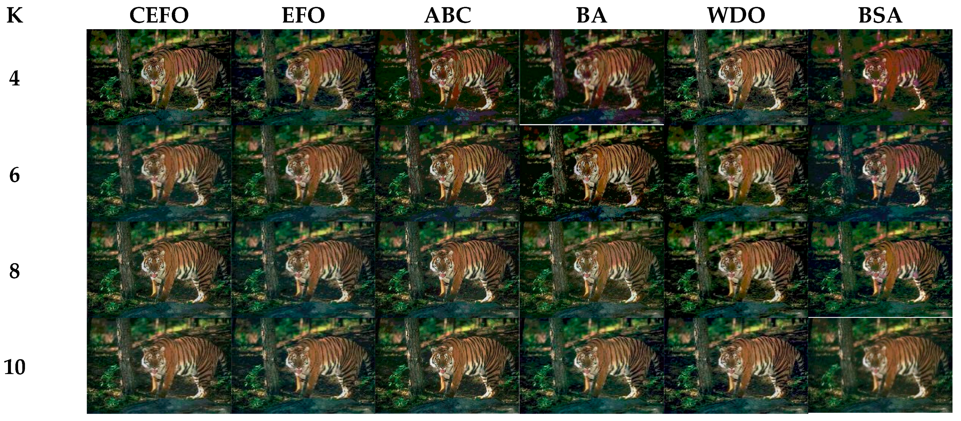
Figure 7.
Segmented images of Test 1 at K = 4, 6, 8, 10 using selected algorithms based on fuzzy entropy.
Figure 7.
Segmented images of Test 1 at K = 4, 6, 8, 10 using selected algorithms based on fuzzy entropy.

Figure 8.
Segmented images of Test 2 at K = 4, 6, 8, 10 using selected algorithms based on fuzzy entropy.
Figure 8.
Segmented images of Test 2 at K = 4, 6, 8, 10 using selected algorithms based on fuzzy entropy.

Figure 9.
Segmented images of Test 3 at K = 4, 6, 8, 10 using selected algorithms based on fuzzy entropy.
Figure 9.
Segmented images of Test 3 at K = 4, 6, 8, 10 using selected algorithms based on fuzzy entropy.

Figure 10.
Segmented images of Test 4 at K = 4, 6, 8, 10 using selected algorithms based on fuzzy entropy.
Figure 10.
Segmented images of Test 4 at K = 4, 6, 8, 10 using selected algorithms based on fuzzy entropy.

Figure 11.
Segmented images of Test 5 at K = 4, 6, 8, 10 using selected algorithms based on fuzzy entropy.
Figure 11.
Segmented images of Test 5 at K = 4, 6, 8, 10 using selected algorithms based on fuzzy entropy.

Figure 12.
Segmented images of Test 6 at K = 4, 6, 8, 10 using selected algorithms based on fuzzy entropy.
Figure 12.
Segmented images of Test 6 at K = 4, 6, 8, 10 using selected algorithms based on fuzzy entropy.

Figure 13.
Segmented images of Test 7 at K = 4, 6, 8, 10 using selected algorithms based on fuzzy entropy.
Figure 13.
Segmented images of Test 7 at K = 4, 6, 8, 10 using selected algorithms based on fuzzy entropy.

Figure 14.
Segmented images of Test 8 at K = 4, 6, 8, 10 using selected algorithms based on fuzzy entropy.
Figure 14.
Segmented images of Test 8 at K = 4, 6, 8, 10 using selected algorithms based on fuzzy entropy.

Figure 15.
Segmented images of Test 9 at K = 4, 6, 8, 10 using selected algorithms based on fuzzy entropy.
Figure 15.
Segmented images of Test 9 at K = 4, 6, 8, 10 using selected algorithms based on fuzzy entropy.

Figure 16.
Segmented images of Test 10 at K = 4, 6, 8, 10 using selected algorithms based on fuzzy entropy.
Figure 16.
Segmented images of Test 10 at K = 4, 6, 8, 10 using selected algorithms based on fuzzy entropy.

Figure 17.
Comparison of Computational Time (CPU Time) based on fuzzy entropy.

Figure 18.
Comparison of Peak Signal to Noise Ratio (PSNR) based on fuzzy entropy.

Figure 19.
Comparison of Mean Structural Similarity (MSSIM) based on fuzzy entropy.

Figure 20.
Comparison of Feature Similarity (FSIM) based on fuzzy entropy.

Figure 21.
Convergence curves of CEFO, EFO, ABC, BA, WDO, and BSA based on fuzzy entropy at K = 10. (Red line represents CEFO; Blue line represents EFO; Cyan line represents ABC; Yellow line represents BA; Magenta line represents WDO; Green ling represents BSA.)
Figure 21.
Convergence curves of CEFO, EFO, ABC, BA, WDO, and BSA based on fuzzy entropy at K = 10. (Red line represents CEFO; Blue line represents EFO; Cyan line represents ABC; Yellow line represents BA; Magenta line represents WDO; Green ling represents BSA.)


Figure 22.
Segmented images at K = 4, 6, 8, 10 using CEFO algorithm based on fuzzy entropy, Otsu’s and Kapur’s entropy.
Figure 22.
Segmented images at K = 4, 6, 8, 10 using CEFO algorithm based on fuzzy entropy, Otsu’s and Kapur’s entropy.


Figure 23.
Comparison of CPU Time based on fuzzy entropy.

Figure 24.
Comparison of PSNR based on fuzzy entropy.

Figure 25.
Comparison of MSSIM based on fuzzy entropy.

Figure 26.
Comparison of FSIM based on fuzzy entropy.


Table 1.
Chaotic maps.
| Name | Chaotic Map |
|---|---|
| Logistic | |
| Sine | |
| Cubic | |
| Circle | |
| Iterative | |
| Tent |
Table 2.
Specific values of parameters used in selected algorithms.
| Algorithm | Parameter | Explanation | Value |
|---|---|---|---|
| EFO | Pfield | The portion of particles belonging to the positive field. | 0.1 |
| Nfield | The portion of particles belonging to the negative field. | 0.45 | |
| Psfield | The probability of selecting electromagnets directly from the positive field. | 0.3 | |
| Rrate | The probability of changing one electromagnet directly from the positive field. | 0.2 | |
| ABC | limit | The value of the max trial limit. | 10 |
| BA | ri | The rate of pulse emission. | [0, 1] |
| Ai | The value of loudness. | [1, 2] | |
| WDO | A constant. | 0.4 | |
| g | The constant of gravitation. | 0.2 | |
| RT | A coefficient. | 3 | |
| Coriolis coefficient. | 0.4 | ||
| BSA | a1, a2 | The values of indirect and direct effects on the birds’ vigilance behaviors. | 2 |
| c1, c2 | The values of the cognitive coefficient and social coefficient. | 2 | |
| FL | The frequency of birds’ flight behaviors. | 0.6 |
Table 3.
Comparison of optimal threshold values between Chaotic Electromagnetic Field Optimization (CEFO) and Electromagnetic Field Optimization (EFO) at K = 4, 6, 8, 10 based on fuzzy entropy.
Table 3.
Comparison of optimal threshold values between Chaotic Electromagnetic Field Optimization (CEFO) and Electromagnetic Field Optimization (EFO) at K = 4, 6, 8, 10 based on fuzzy entropy.
| Image | K | CEFO | EFO | ||||
|---|---|---|---|---|---|---|---|
| R | G | B | R | G | B | ||
| Test 1 | 4 | 56 93 153 187 | 57 88 132 191 | 59 10 157 197 | 61 90 144 188 | 18 74 115 170 | 58 87 148 202 |
| 6 | 20 59 92 128 167 199 | 26 47 81 114 161 203 | 25 48 76 111 138 195 | 26 60 95 128 162 198 | 19 47 80 119 171 210 | 18 57 85 122 154 212 | |
| 8 | 11 31 58 82 107 132 168 211 | 12 42 64 92 114 149 181 210 | 18 50 73 97 143 168 196 223 | 17 47 71 90 115 138 171 209 | 12 39 67 93 130 170 205 223 | 26 56 78 100 113 162 190 216 | |
| 10 | 14 37 55 75 90 111 130 159 182 210 | 11 41 61 95 122 146 168 185 208 237 | 14 40 64 80 105 136 161 189 212 231 | 10 26 56 82 102 133 148 167 192 215 | 11 32 59 76 90 107 134 166 198 222 | 24 41 56 72 93 126 156 181 203 229 | |
| Test 2 | 4 | 10 93 114 171 | 86 143 194 226 | 91 110 137 189 | 80 116 149 183 | 93 113 146 216 | 104 124 170 206 |
| 6 | 18 41 75 107 147 177 | 87 101 133 153 192 234 | 54 72 97 121 156 192 | 73 83 108 139 176 219 | 94 114 135 162 197 231 | 16 50 85 129 156 199 | |
| 8 | 15 27 44 59 96 127 171 204 | 14 22 43 65 117 144 190 222 | 39 61 82 117 148 176 195 223 | 7 34 55 78 107 135 166 199 | 49 65 76 139 168 193 211 232 | 45 61 82 101 129 154 182 213 | |
| 10 | 32 55 75 108 144 171 195 215 226 239 | 5 50 65 85 102 121 139 167 197 228 | 31 47 64 87 108 125 158 179 209 239 | 4 24 47 67 102 122 147 180 204 223 | 19 33 53 71 99 119 144 170 195 224 | 19 36 57 80 108 141 154 177 201 230 | |
| Test 3 | 4 | 44 92 139 188 | 31 92 139 188 | 27 97 138 185 | 33 80 126 181 | 37 87 142 206 | 29 106 154 188 |
| 6 | 32 62 93 128 173 199 | 19 53 90 119 162 206 | 36 71 105 136 183 208 | 32 76 116 150 177 207 | 50 69 101 143 190 216 | 15 46 70 113 153 197 | |
| 8 | 22 43 68 91 112 138 172 208 | 17 51 73 98 123 148 181 207 | 11 36 58 88 106 141 170 213 | 19 54 94 125 141 164 190 214 | 25 49 72 96 126 156 192 223 | 15 49 71 95 128 159 187 214 | |
| 10 | 26 39 55 69 86 110 131 154 175 207 | 42 29 56 79 104 121 141 163 197 219 | 9 25 49 82 109 132 154 176 199 222 | 17 31 45 62 93 124 168 194 212 229 | 14 39 56 76 95 114 148 176 196 224 | 16 13 34 58 82 115 150 180 199 223 | |
| Test 4 | 4 | 52 84 127 164 | 67 102 141 204 | 49 74 111 155 | 59 88 129 164 | 64 105 153 199 | 61 101 145 203 |
| 6 | 38 62 97 137 172 195 | 48 71 111 144 175 213 | 43 77 109 147 178 235 | 40 65 89 112 147 184 | 44 67 105 126 167 211 | 39 63 98 134 160 190 | |
| 8 | 13 31 54 92 110 142 175 198 | 35 60 86 114 137 169 200 226 | 24 41 64 94 129 156 193 224 | 15 26 46 68 97 134 160 189 | 18 43 73 100 128 155 190 225 | 23 57 105 137 169 195 221 237 | |
| 10 | 6 25 43 64 84 106 132 152 172 189 | 7 27 39 52 75 99 130 157 190 221 | 15 25 48 78 103 130 157 178 219 240 | 8 18 31 48 74 100 124 153 181 211 | 8 23 39 57 80 104 127 157 188 215 | 10 27 50 87 117 146 171 194 218 234 | |
| Test 5 | 4 | 52 98 149 198 | 55 89 164 215 | 77 125 162 209 | 87 122 152 190 | 38 58 106 162 | 80 120 160 194 |
| 6 | 22 63 93 131 179 225 | 16 69 97 125 158 204 | 15 61 97 131 166 207 | 23 64 90 140 183 213 | 26 75 114 134 169 211 | 20 59 84 132 169 205 | |
| 8 | 16 59 77 94 116 134 162 199 | 20 58 75 98 129 155 185 214 | 19 56 77 115 145 173 196 227 | 14 56 75 104 127 162 191 225 | 37 37 60 76 111 135 175 214 | 17 39 66 97 122 171 205 234 | |
| 10 | 13 29 57 77 93 107 130 165 188 214 | 14 30 62 78 94 126 152 179 205 231 | 19 44 56 72 89 109 129 159 176 205 | 11 26 50 72 92 115 149 180 201 224 | 16 25 48 64 85 106 127 142 175 206 | 24 41 56 70 96 123 150 177 202 229 | |
| Test 6 | 4 | 55 97 158 195 | 64 99 153 190 | 46 75 131 179 | 52 100 144 192 | 56 92 123 178 | 52 88 149 176 |
| 6 | 43 60 91 118 165 202 | 25 38 76 119 165 205 | 47 69 97 133 155 190 | 44 75 112 150 176 211 | 60 87 109 135 167 196 | 32 51 85 125 172 207 | |
| 8 | 16 42 73 91 129 157 190 221 | 10 34 52 79 108 136 168 207 | 23 39 64 86 120 137 172 202 | 28 45 74 91 120 150 191 225 | 15 26 55 85 111 141 176 205 | 23 38 57 87 119 159 183 214 | |
| 10 | 10 32 50 77 99 134 162 192 209 228 | 13 36 47 69 107 140 164 185 200 223 | 14 33 60 82 101 130 156 183 208 228 | 8 30 46 72 99 125 145 166 189 221 | 10 28 53 72 100 125 146 172 187 206 | 14 31 51 68 86 115 134 167 190 221 | |
| Test 7 | 4 | 66 95 139 176 | 25 66 108 157 | 23 88 134 220 | 26 89 132 179 | 43 89 133 178 | 30 94 137 208 |
| 6 | 17 33 80 120 168 205 | 20 80 108 133 164 189 | 13 59 84 102 128 151 | 20 41 60 92 131 180 | 21 54 86 111 144 183 | 31 67 101 138 196 223 | |
| 8 | 20 54 79 106 126 146 169 209 | 13 50 80 102 132 166 197 223 | 19 40 63 88 119 148 200 228 | 14 58 80 98 122 146 167 207 | 18 55 82 105 128 161 193 228 | 18 36 67 91 128 149 200 220 | |
| 10 | 10 30 41 63 89 110 129 154 178 216 | 14 54 68 82 106 132 169 197 220 243 | 15 41 66 85 105 133 151 190 214 233 | 12 28 59 82 115 146 179 199 215 227 | 12 31 57 76 92 117 141 168 200 223 | 10 34 63 95 120 140 157 185 212 232 | |
| Test 8 | 4 | 48 73 173 212 | 62 107 141 207 | 43 79 124 215 | 22 83 139 199 | 55 105 149 201 | 37 102 183 234 |
| 6 | 38 64 101 141 181 224 | 32 61 85 126 155 196 | 38 61 91 126 197 218 | 40 66 96 151 182 212 | 40 66 97 140 175 209 | 34 54 88 117 182 230 | |
| 8 | 15 41 64 85 110 133 175 213 | 44 34 74 110 135 158 179 203 | 25 40 69 104 136 182 207 231 | 31 55 77 93 108 135 178 217 | 25 51 80 117 155 179 206 227 | 30 32 60 103 117 141 179 215 | |
| 10 | 18 39 58 87 115 137 172 186 210 230 | 21 36 63 79 111 129 150 180 208 227 | 28 47 74 90 116 131 153 178 208 226 | 22 42 69 84 109 133 158 182 208 227 | 39 91 103 127 146 159 176 193 208 225 | 21 35 65 98 119 140 165 184 211 231 | |
| Test 9 | 4 | 47 74 107 149 | 55 90 132 167 | 42 66 117 149 | 33 67 109 155 | 53 87 123 165 | 45 89 155 211 |
| 6 | 13 43 62 92 126 165 | 15 50 89 125 160 195 | 19 45 81 115 151 230 | 12 42 59 96 127 160 | 24 33 76 115 143 190 | 28 48 80 116 149 167 | |
| 8 | 14 36 53 75 92 123 152 173 | 11 40 55 77 101 126 151 183 | 26 41 66 91 128 155 200 233 | 11 38 54 81 115 139 166 187 | 17 66 86 105 125 145 172 197 | 28 51 76 104 132 154 172 207 | |
| 10 | 13 23 41 59 82 106 126 158 181 198 | 11 43 54 72 89 105 134 163 188 213 | 24 47 71 94 118 140 160 177 208 237 | 9 41 60 92 116 131 150 167 185 203 | 13 30 47 67 86 108 131 150 183 212 | 20 43 71 92 115 155 175 190 226 240 | |
| Test 10 | 4 | 48 76 132 175 | 31 69 117 169 | 53 86 116 200 | 62 101 132 190 | 45 70 123 186 | 52 83 139 193 |
| 6 | 34 57 90 127 166 196 | 53 90 116 142 180 214 | 42 56 104 136 169 220 | 33 56 87 127 162 198 | 43 76 118 155 190 225 | 42 70 100 133 164 226 | |
| 8 | 19 33 62 91 133 165 195 214 | 20 26 57 90 112 150 195 220 | 12 38 55 88 113 150 186 229 | 34 60 98 128 148 170 194 221 | 17 38 58 87 119 147 187 216 | 10 23 49 79 121 149 170 189 | |
| 10 | 16 35 54 71 93 119 141 169 196 231 | 9 26 36 51 72 106 132 166 195 224 | 10 26 41 61 77 108 134 160 185 213 | 14 33 56 86 106 129 159 189 212 235 | 8 29 43 75 99 118 141 168 196 226 | 10 33 48 69 90 113 144 169 194 230 | |
Table 4.
Comparison of optimal threshold values between Artificial Bee Colony (ABC) and Bat Algorithm (BA) at K = 4, 6, 8, 10 based on fuzzy entropy.
Table 4.
Comparison of optimal threshold values between Artificial Bee Colony (ABC) and Bat Algorithm (BA) at K = 4, 6, 8, 10 based on fuzzy entropy.
| Image | K | ABC | BA | ||||
|---|---|---|---|---|---|---|---|
| R | G | B | R | G | B | ||
| Test 1 | 4 | 55 103 154 201 | 69 104 156 207 | 40 96 165 219 | 49 78 150 214 | 66 92 128 195 | 78 116 176 213 |
| 6 | 24 63 109 149 184 220 | 47 74 111 152 183 218 | 39 84 126 154 188 220 | 31 58 81 105 150 195 | 20 45 85 115 165 212 | 29 71 118 154 190 230 | |
| 8 | 24 51 81 113 142 177 211 226 | 20 54 77 108 150 174 200 223 | 15 47 75 107 143 171 207 237 | 12 51 80 98 117 155 193 225 | 13 48 77 109 159 181 205 225 | 33 63 94 110 143 168 203 242 | |
| 10 | 16 41 59 85 113 142 167 187 211 236 | 15 43 62 88 112 139 167 189 209 232 | 13 39 62 83 113 139 165 192 221 236 | 20 50 82 99 125 149 168 190 211 231 | 15 41 88 107 129 146 158 177 206 232 | 31 51 72 84 99 129 162 191 227 242 | |
| Test 2 | 4 | 63 108 164 216 | 78 119 159 231 | 72 98 171 224 | 117 150 188 275 | 129 152 182 231 | 88 113 140 189 |
| 6 | 49 76 112 149 196 236 | 52 79 125 159 189 223 | 56 78 124 148 182 219 | 81 107 143 173 205 232 | 83 97 112 130 212 233 | 83 114 153 178 206 238 | |
| 8 | 38 51 73 110 143 182 221 240 | 37 56 90 122 143 170 195 222 | 31 51 79 109 149 175 207 246 | 35 48 68 89 140 181 210 236 | 51 85 120 156 182 214 242 250 | 5 20 45 82 113 149 177 217 | |
| 10 | 22 37 57 85 112 142 167 192 223 237 | 6 45 60 80 109 133 160 188 218 244 | 23 40 65 88 115 144 163 188 218 239 | 64 69 75 81 98 120 155 187 210 230 | 30 50 70 92 120 147 171 193 214 238 | 28 58 79 98 135 162 186 206 234 248 | |
| Test 3 | 4 | 31 103 162 206 | 60 102 151 209 | 44 103 157 206 | 53 99 141 197 | 53 121 164 203 | 23 100 143 191 |
| 6 | 34 68 103 140 190 226 | 29 66 101 140 186 217 | 31 67 98 138 186 217 | 29 66 116 154 185 215 | 39 72 122 154 181 210 | 45 86 116 143 173 219 | |
| 8 | 18 51 79 111 138 173 205 232 | 28 56 84 108 140 168 194 231 | 20 50 77 103 141 168 199 222 | 20 43 75 97 136 181 205 236 | 25 51 80 108 136 177 203 231 | 12 56 86 110 138 175 202 227 | |
| 10 | 19 37 63 87 112 137 170 195 222 244 | 22 46 65 92 118 141 165 194 216 237 | 21 52 71 96 110 136 157 196 214 230 | 19 40 64 90 117 147 174 206 227 244 | 36 62 88 105 116 135 162 196 216 239 | 30 51 74 100 113 135 146 160 184 214 | |
| Test 4 | 4 | 40 90 136 172 | 63 118 170 210 | 63 96 146 208 | 68 110 141 168 | 60 112 161 208 | 49 109 189 234 |
| 6 | 32 69 114 155 190 219 | 42 66 111 161 201 237 | 35 65 104 146 186 235 | 38 59 116 147 173 197 | 37 78 135 168 193 223 | 40 74 108 137 155 226 | |
| 8 | 21 45 78 107 137 169 206 227 | 32 56 83 120 142 177 212 241 | 26 49 80 116 156 182 213 233 | 8 36 61 92 125 197 222 241 | 26 52 84 112 135 160 198 228 | 26 58 91 121 146 170 198 228 | |
| 10 | 25 45 60 84 114 140 168 191 217 232 | 26 43 62 86 108 136 161 191 216 245 | 22 38 63 85 113 137 159 193 223 241 | 8 33 64 96 128 156 174 195 217 234 | 38 63 84 105 129 145 168 192 206 231 | 25 41 54 67 96 130 152 186 209 233 | |
| Test 5 | 4 | 34 94 167 222 | 29 93 159 220 | 75 118 169 231 | 33 107 160 196 | 29 75 134 225 | 72 106 149 208 |
| 6 | 26 72 97 138 187 223 | 21 73 108 140 188 226 | 20 71 118 153 191 231 | 59 86 122 163 202 228 | 19 62 94 144 184 234 | 52 101 136 176 213 234 | |
| 8 | 16 52 84 117 141 175 202 229 | 13 62 86 117 143 178 203 228 | 18 56 77 103 135 172 200 234 | 27 61 85 117 142 171 201 238 | 89 124 141 157 171 183 198 225 | 56 78 98 126 157 167 199 234 | |
| 10 | 18 36 68 99 124 147 167 183 206 228 | 12 50 68 88 114 144 169 192 219 238 | 18 41 65 92 111 133 163 190 220 241 | 17 37 54 72 104 138 160 178 191 231 | 14 68 86 104 118 141 168 197 216 231 | 16 43 68 98 128 154 177 198 220 241 | |
| Test 6 | 4 | 72 116 162 197 | 59 92 142 177 | 60 91 143 196 | 60 121 178 210 | 55 91 135 174 | 59 94 128 166 |
| 6 | 35 54 103 142 184 222 | 31 66 111 161 192 228 | 36 74 114 158 197 218 | 12 59 96 121 156 201 | 61 110 147 175 204 233 | 44 74 103 131 190 227 | |
| 8 | 16 45 79 113 151 189 210 231 | 13 51 85 119 156 182 212 234 | 21 44 84 120 148 176 206 224 | 13 33 48 60 119 152 190 236 | 41 64 98 119 158 183 203 222 | 11 40 62 125 165 183 213 234 | |
| 10 | 15 42 60 86 114 144 164 194 214 231 | 11 41 60 81 101 130 155 181 212 233 | 26 46 64 80 110 131 164 185 201 220 | 11 47 75 102 121 134 150 178 204 227 | 14 39 58 84 108 138 161 186 210 235 | 21 38 51 71 90 115 144 172 191 228 | |
| Test 7 | 4 | 55 97 147 210 | 45 96 148 216 | 41 92 139 220 | 67 96 125 171 | 84 112 163 244 | 24 76 173 219 |
| 6 | 33 72 111 153 177 219 | 19 75 110 147 181 227 | 25 71 109 148 190 227 | 57 75 92 122 166 212 | 27 87 118 141 185 234 | 21 67 100 140 192 235 | |
| 8 | 24 59 79 102 129 157 188 221 | 29 65 87 113 145 166 195 231 | 24 56 86 113 147 189 211 234 | 41 72 92 116 138 154 169 212 | 22 45 79 104 133 162 200 226 | 14 45 72 111 154 188 212 244 | |
| 10 | 15 39 68 98 125 142 166 195 220 237 | 13 40 69 87 110 140 170 202 223 242 | 17 44 71 89 113 138 158 193 214 234 | 21 62 94 122 144 163 183 200 217 242 | 43 80 102 121 140 159 175 196 223 237 | 20 50 84 111 131 167 180 205 223 239 | |
| Test 8 | 4 | 55 86 183 220 | 60 104 153 225 | 33 85 121 226 | 32 78 163 226 | 63 106 148 222 | 54 97 126 192 |
| 6 | 38 82 126 154 193 229 | 44 74 114 152 181 230 | 35 57 76 105 130 235 | 46 87 148 181 215 237 | 53 78 119 144 184 227 | 27 42 65 90 112 141 | |
| 8 | 14 48 81 105 142 175 212 239 | 24 55 90 116 146 174 208 236 | 29 62 80 110 133 172 208 236 | 28 71 98 124 149 179 204 233 | 24 54 81 104 142 177 211 236 | 9 21 42 84 113 132 192 240 | |
| 10 | 11 34 57 78 101 133 167 191 216 234 | 17 35 64 85 109 134 155 183 210 239 | 20 40 72 99 116 135 167 186 218 240 | 16 51 79 103 126 144 169 194 224 239 | 18 50 66 83 101 121 147 172 207 227 | 18 47 82 105 127 145 169 194 220 240 | |
| Test 9 | 4 | 64 110 138 182 | 43 96 149 194 | 52 101 145 221 | 68 104 122 151 | 35 73 109 182 | 38 92 144 208 |
| 6 | 19 62 101 131 157 197 | 39 74 106 145 183 212 | 30 65 102 135 166 234 | 39 63 90 116 141 181 | 12 51 100 129 161 198 | 40 54 72 101 129 158 | |
| 8 | 21 56 98 134 154 173 194 214 | 16 43 67 99 141 175 197 216 | 22 50 83 115 146 168 205 239 | 38 58 74 104 128 145 175 198 | 40 60 105 141 163 187 213 236 | 15 29 60 96 126 167 210 239 | |
| 10 | 12 42 63 87 114 141 169 197 223 238 | 15 46 66 86 110 137 160 187 214 236 | 25 45 60 85 111 136 164 193 227 242 | 23 66 88 123 142 154 164 179 199 216 | 14 42 64 84 111 135 159 184 203 226 | 16 32 48 99 135 158 174 202 227 243 | |
| Test 10 | 4 | 58 104 164 221 | 70 110 161 213 | 77 122 159 215 | 74 134 165 199 | 70 109 164 238 | 78 104 163 193 |
| 6 | 38 76 125 159 192 229 | 53 79 111 139 176 218 | 48 71 101 135 182 221 | 26 80 137 166 196 233 | 51 96 118 138 169 209 | 42 74 121 155 198 229 | |
| 8 | 31 49 76 110 142 169 202 240 | 32 52 86 117 148 180 206 226 | 29 52 83 114 146 171 195 234 | 32 67 94 119 147 174 199 240 | 47 75 90 103 117 159 187 219 | 35 67 108 136 162 185 215 243 | |
| 10 | 27 47 69 94 120 143 164 185 212 242 | 26 43 66 95 117 142 165 192 221 239 | 22 39 62 89 110 135 157 185 214 238 | 33 66 88 111 125 143 156 180 201 239 | 11 29 53 84 114 136 166 193 220 234 | 13 39 58 105 132 166 183 207 230 247 | |
Table 5.
Comparison of optimal threshold values between Wind Driven Optimization (WDO) and Bird Swarm Algorithm (BSA) at K = 4, 6, 8, 10 based on fuzzy entropy.
Table 5.
Comparison of optimal threshold values between Wind Driven Optimization (WDO) and Bird Swarm Algorithm (BSA) at K = 4, 6, 8, 10 based on fuzzy entropy.
| Image | K | WDO | BSA | ||||
|---|---|---|---|---|---|---|---|
| R | G | B | R | G | B | ||
| Test 1 | 4 | 68 107 150 192 | 65 103 156 198 | 77 115 164 196 | 54 119 190 243 | 12 57 174 243 | 24 93 175 238 |
| 6 | 44 74 109 134 172 205 | 53 84 120 149 175 205 | 61 95 131 154 186 218 | 22 90 100 165 239 255 | 6 30 78 158 214 239 | 35 58 93 153 186 227 | |
| 8 | 47 72 101 121 144 168 188 211 | 48 75 104 129 149 170 192 213 | 46 68 91 110 131 156 174 212 | 7 57 108 118 129 158 216 251 | 9 55 68 97 181 209 241 255 | 4 32 78 123 152 179 196 247 | |
| 10 | 45 67 93 115 131 142 161 176 194 210 | 51 65 82 98 114 133 152 171 195 217 | 25 45 65 80 95 113 139 164 194 223 | 12 27 46 70 102 136 153 178 198 228 | 17 37 49 72 95 132 155 194 213 226 | 12 33 63 99 132 161 189 212 228 243 | |
| Test 2 | 4 | 123 146 174 202 | 128 154 183 216 | 98 131 170 208 | 7 39 194 232 | 24 112 145 227 | 71 105 128 183 |
| 6 | 100 117 138 160 185 205 | 109 129 153 171 195 225 | 87 103 128 164 181 214 | 17 51 79 129 191 230 | 3 18 55 104 145 223 | 26 70 90 142 217 240 | |
| 8 | 78 93 104 118 134 146 169 200 | 93 111 131 147 165 182 202 228 | 62 74 92 111 131 154 179 211 | 17 52 83 123 181 216 230 247 | 18 73 92 119 152 190 225 252 | 59 90 102 121 142 198 224 240 | |
| 10 | 70 82 95 107 122 134 150 168 189 209 | 80 90 101 112 120 130 142 157 170 190 | 70 83 103 118 137 147 166 182 200 218 | 1 20 75 79 82 87 118 142 179 211 | 16 38 73 114 130 163 196 248 253 255 | 22 73 90 123 137 148 179 205 215 239 | |
| Test 3 | 4 | 48 104 158 199 | 68 121 163 196 | 77 119 161 201 | 39 94 147 214 | 42 117 173 201 | 24 107 208 221 |
| 6 | 44 80 113 148 176 212 | 47 77 105 141 180 214 | 56 83 114 136 168 211 | 62 96 128 176 199 223 | 16 42 63 76 122 219 | 12 34 67 126 183 212 | |
| 8 | 37 67 92 112 135 163 189 217 | 38 59 82 102 129 156 188 213 | 46 70 91 117 140 162 190 213 | 1 37 51 77 115 159 209 237 | 19 60 102 149 177 203 223 251 | 20 57 73 95 125 159 188 221 | |
| 10 | 36 69 100 120 142 156 172 190 204 223 | 30 54 73 96 119 137 158 178 198 222 | 24 49 67 83 104 120 143 170 192 214 | 8 77 109 140 164 179 202 207 231 254 | 1 25 82 98 109 164 178 196 230 255 | 17 56 80 97 119 146 172 216 229 251 | |
| Test 4 | 4 | 54 94 132 169 | 71 117 154 200 | 78 109 147 207 | 46 89 145 214 | 18 95 184 244 | 36 77 130 213 |
| 6 | 49 72 101 128 156 183 | 58 87 109 143 181 212 | 51 89 115 152 194 223 | 35 52 85 128 167 193 | 41 70 93 146 203 231 | 18 54 89 128 169 221 | |
| 8 | 40 67 94 120 139 156 176 193 | 48 73 93 118 138 166 196 225 | 45 76 106 129 153 176 205 229 | 1 3 30 81 120 181 218 237 | 26 56 92 133 185 205 224 244 | 23 42 91 133 163 204 223 236 | |
| 10 | 41 59 83 103 124 141 151 167 185 198 | 44 64 81 100 115 134 155 175 199 223 | 43 67 86 103 123 141 159 176 198 227 | 13 26 41 66 92 119 147 190 226 246 | 23 54 74 99 123 145 167 190 216 240 | 15 26 59 95 113 130 156 183 212 238 | |
| Test 5 | 4 | 86 123 161 198 | 88 123 165 203 | 78 118 159 199 | 8 55 142 203 | 82 107 159 198 | 22 57 114 226 |
| 6 | 71 90 116 154 188 218 | 78 103 127 157 186 211 | 65 101 133 162 190 222 | 42 106 138 203 227 253 | 11 41 110 152 204 248 | 75 133 164 194 214 237 | |
| 8 | 33 67 88 114 131 158 183 212 | 59 76 97 114 135 164 192 222 | 58 78 97 121 142 168 192 227 | 11 33 86 110 175 195 211 247 | 3 63 123 177 197 216 239 255 | 26 54 85 123 150 178 211 230 | |
| 10 | 57 77 100 116 132 148 166 181 201 223 | 36 52 70 88 109 128 146 160 183 201 | 64 87 101 115 128 144 161 179 196 217 | 32 46 62 94 121 149 171 188 209 238 | 8 21 50 87 104 138 148 166 192 229 | 9 36 88 110 123 142 163 182 216 249 | |
| Test 6 | 4 | 59 104 157 197 | 69 106 147 193 | 59 100 130 177 | 25 127 153 246 | 16 78 149 224 | 28 98 172 231 |
| 6 | 54 81 108 141 175 202 | 55 83 115 151 177 209 | 41 71 104 137 163 199 | 36 100 122 148 178 204 | 29 87 116 142 163 198 | 13 28 69 91 137 228 | |
| 8 | 45 74 100 123 146 167 191 215 | 55 81 105 131 151 171 191 213 | 38 67 92 122 142 169 186 211 | 8 52 79 123 158 181 210 243 | 11 50 109 132 169 204 219 234 | 20 63 104 130 137 168 207 246 | |
| 10 | 37 53 73 90 110 131 147 170 197 222 | 47 69 89 105 128 143 162 179 197 219 | 36 61 83 99 118 137 157 175 199 216 | 23 42 60 77 108 132 152 182 218 235 | 6 33 61 108 126 158 180 207 228 245 | 14 71 105 126 149 173 208 219 230 244 | |
| Test 7 | 4 | 74 110 145 176 | 85 107 145 184 | 75 100 136 182 | 28 95 224 255 | 43 70 135 235 | 46 134 198 247 |
| 6 | 63 84 114 143 170 201 | 22 76 100 132 169 221 | 48 79 107 130 151 191 | 7 30 49 115 157 194 | 30 71 107 144 183 242 | 4 55 137 166 205 251 | |
| 8 | 41 68 97 120 139 165 184 216 | 43 76 97 119 140 164 181 220 | 34 57 82 109 129 151 200 233 | 16 37 65 85 108 141 169 222 | 13 44 70 118 144 157 177 236 | 13 57 95 117 145 183 214 230 | |
| 10 | 53 70 89 109 122 141 159 176 195 217 | 25 44 66 81 103 123 142 158 180 227 | 55 80 105 123 133 144 156 164 184 234 | 14 35 57 75 88 120 141 154 173 214 | 11 38 58 76 100 126 149 172 189 240 | 17 37 74 100 124 155 175 210 227 242 | |
| Test 8 | 4 | 69 124 160 207 | 62 118 152 207 | 44 92 122 189 | 48 83 156 213 | 22 81 125 216 | 61 98 114 212 |
| 6 | 50 85 114 157 184 213 | 54 85 116 149 176 216 | 38 71 103 128 192 221 | 6 31 73 108 214 254 | 49 103 122 161 190 235 | 14 55 109 163 195 234 | |
| 8 | 41 61 86 111 136 161 188 220 | 41 67 88 110 130 157 193 224 | 38 68 91 105 123 140 184 232 | 21 41 67 76 107 134 163 231 | 21 47 88 119 159 194 221 242 | 12 37 67 116 137 160 184 235 | |
| 10 | 34 47 68 88 112 132 157 180 214 236 | 45 70 89 108 125 137 152 164 178 206 | 28 42 55 76 104 132 167 194 210 230 | 15 38 76 102 125 160 178 209 224 243 | 10 33 46 73 101 138 162 204 227 242 | 33 47 68 93 114 132 142 153 177 213 | |
| Test 9 | 4 | 70 104 138 160 | 71 106 142 176 | 58 107 149 225 | 47 86 157 234 | 43 92 125 219 | 37 92 147 223 |
| 6 | 57 82 110 133 156 177 | 61 92 116 137 163 187 | 43 74 102 126 155 206 | 41 93 139 167 213 221 | 13 79 118 156 166 205 | 11 71 112 155 175 239 | |
| 8 | 50 72 97 120 138 155 172 190 | 54 75 93 110 131 151 173 194 | 37 62 91 121 143 165 205 219 | 3 19 32 70 111 155 188 227 | 11 35 76 122 141 181 216 230 | 23 74 94 113 147 189 214 241 | |
| 10 | 49 64 79 92 105 118 137 158 173 191 | 50 69 90 108 121 139 155 170 187 204 | 38 67 85 98 113 129 145 164 196 222 | 7 35 69 99 115 136 157 184 210 251 | 5 17 37 91 113 158 202 229 247 252 | 25 57 90 112 141 155 174 196 216 232 | |
| Test 10 | 4 | 62 89 136 179 | 70 103 136 191 | 70 111 156 191 | 32 132 173 217 | 37 90 134 215 | 70 129 166 192 |
| 6 | 52 93 129 155 187 226 | 54 88 116 148 184 216 | 50 80 111 141 171 207 | 51 85 123 155 187 218 | 14 33 61 117 187 237 | 41 67 108 139 182 219 | |
| 8 | 35 66 89 107 136 164 188 219 | 49 72 96 117 141 167 198 223 | 47 67 89 117 143 166 193 224 | 21 53 63 86 123 185 213 236 | 19 56 78 112 143 186 238 253 | 11 44 70 123 154 173 193 215 | |
| 10 | 41 67 90 114 131 153 174 200 215 232 | 41 62 80 96 109 128 139 157 189 227 | 41 61 81 102 121 136 158 172 199 232 | 19 37 65 91 104 134 165 194 223 246 | 29 50 74 98 114 137 161 190 226 240 | 6 28 57 105 132 157 180 199 224 239 | |
Table 6.
Comparison of CPU Time (in seconds) and PSNR computed by CEFO, EFO, ABC, BA, WDO, and BSA using fuzzy entropy. The bold numbers are the best values in the relevant index.
Table 6.
Comparison of CPU Time (in seconds) and PSNR computed by CEFO, EFO, ABC, BA, WDO, and BSA using fuzzy entropy. The bold numbers are the best values in the relevant index.
| Image | K | Computational Time (CPU Time) | Peak Signal to Noise Ratio (PSNR) | ||||||||||
|---|---|---|---|---|---|---|---|---|---|---|---|---|---|
| CEFO | EFO | ABC | BA | WDO | BSA | CEFO | EFO | ABC | BA | WDO | BSA | ||
| Test 1 | 4 | 0.17541 | 0.20379 | 5.13759 | 2.45288 | 2.49367 | 2.97138 | 19.0869 | 18.5304 | 17.8020 | 17.3212 | 15.9576 | 16.8238 |
| 6 | 0.21623 | 0.26617 | 6.63971 | 2.98102 | 3.04503 | 3.33423 | 22.4966 | 21.0851 | 20.8826 | 19.4872 | 19.2521 | 19.3995 | |
| 8 | 0.26219 | 0.30416 | 7.40398 | 3.54215 | 3.53203 | 3.96657 | 23.9315 | 23.3153 | 23.0079 | 23.0902 | 21.2553 | 21.9558 | |
| 10 | 0.33284 | 0.35769 | 8.54834 | 4.05983 | 4.12060 | 4.61008 | 25.1603 | 24.8085 | 24.9762 | 23.5623 | 23.5174 | 24.2976 | |
| Test 2 | 4 | 0.18152 | 0.19745 | 5.48045 | 2.62491 | 2.55021 | 3.05768 | 18.5011 | 16.6384 | 17.9217 | 14.9956 | 14.6621 | 16.8609 |
| 6 | 0.23014 | 0.25140 | 6.52806 | 2.98864 | 3.11644 | 3.67576 | 21.4186 | 20.8410 | 21.4261 | 17.9962 | 16.1975 | 22.5361 | |
| 8 | 0.26745 | 0.30171 | 7.39266 | 3.54545 | 3.54003 | 4.00924 | 23.4745 | 23.5633 | 24.0574 | 18.3652 | 19.0371 | 22.6106 | |
| 10 | 0.35415 | 0.36493 | 8.32270 | 4.07706 | 4.17821 | 4.71338 | 27.1960 | 26.5362 | 26.5537 | 24.7670 | 19.9620 | 22.7476 | |
| Test 3 | 4 | 0.19354 | 0.20952 | 5.42962 | 2.54004 | 2.32354 | 3.05836 | 17.9266 | 18.0706 | 17.7559 | 15.0795 | 17.8259 | 16.1882 |
| 6 | 0.24406 | 0.27724 | 6.51639 | 3.07212 | 3.14887 | 3.21041 | 21.4595 | 20.9724 | 21.0554 | 20.6465 | 20.9096 | 18.7586 | |
| 8 | 0.26572 | 0.30195 | 7.43254 | 3.61201 | 3.64706 | 4.05836 | 23.5257 | 22.7557 | 22.9832 | 22.7031 | 23.0729 | 21.4050 | |
| 10 | 0.31104 | 0.35756 | 8.49756 | 4.05537 | 4.27057 | 4.97929 | 25.1107 | 24.1796 | 24.6243 | 23.9076 | 24.8630 | 21.4820 | |
| Test 4 | 4 | 0.20654 | 0.22286 | 5.22364 | 2.53570 | 2.51094 | 2.89167 | 18.5791 | 18.5562 | 18.4538 | 17.8594 | 18.1050 | 18.4835 |
| 6 | 0.25613 | 0.27055 | 6.52943 | 3.00267 | 3.05336 | 3.40388 | 21.9962 | 21.5752 | 21.4728 | 21.0931 | 20.4419 | 21.3494 | |
| 8 | 0.29565 | 0.31734 | 7.34861 | 3.53905 | 3.74083 | 4.08592 | 23.6574 | 22.9513 | 22.5091 | 22.4950 | 22.1239 | 21.8930 | |
| 10 | 0.34226 | 0.43022 | 8.48234 | 4.19234 | 4.20027 | 4.77867 | 24.8212 | 24.7081 | 24.3937 | 24.5774 | 23.1124 | 24.5733 | |
| Test 5 | 4 | 0.20017 | 0.22525 | 5.27645 | 2.53857 | 2.48718 | 2.98304 | 18.0239 | 17.6242 | 16.8089 | 16.3870 | 17.3516 | 15.8329 |
| 6 | 0.25485 | 0.26024 | 6.89415 | 3.06993 | 3.06272 | 3.53148 | 20.3479 | 20.4329 | 20.0547 | 20.2630 | 19.1668 | 18.4271 | |
| 8 | 0.29424 | 0.32101 | 7.55179 | 3.86221 | 3.68722 | 4.09332 | 22.1661 | 21.8127 | 22.1693 | 21.5206 | 21.5001 | 19.8220 | |
| 10 | 0.34480 | 0.35174 | 8.37159 | 4.09532 | 4.24325 | 4.95875 | 24.0138 | 23.7462 | 23.8704 | 23.4936 | 22.2399 | 23.5245 | |
| Test 6 | 4 | 0.19472 | 0.20841 | 5.12137 | 2.49369 | 2.53905 | 3.08066 | 18.1095 | 17.6491 | 17.6509 | 17.7857 | 17.7293 | 16.8704 |
| 6 | 0.24263 | 0.26745 | 6.57661 | 3.07078 | 3.06447 | 3.58303 | 21.4831 | 20.6287 | 21.0117 | 20.2254 | 20.2431 | 19.4964 | |
| 8 | 0.30864 | 0.32049 | 7.35641 | 3.57464 | 3.50718 | 4.12885 | 23.2290 | 23.3256 | 22.7773 | 21.8122 | 21.4135 | 20.8800 | |
| 10 | 0.33725 | 0.35708 | 8.54900 | 4.03751 | 4.15783 | 4.86694 | 24.7681 | 24.4737 | 24.5259 | 24.6509 | 23.1793 | 22.5603 | |
| Test 7 | 4 | 0.20678 | 0.23005 | 5.22556 | 2.53131 | 2.44727 | 3.00952 | 18.8739 | 18.5039 | 18.0277 | 16.4128 | 16.4863 | 16.0152 |
| 6 | 0.23562 | 0.25809 | 6.62490 | 3.07199 | 3.21664 | 3.41591 | 22.1443 | 21.6213 | 20.0762 | 19.9806 | 20.8248 | 18.3119 | |
| 8 | 0.29807 | 0.30283 | 7.41492 | 3.56056 | 3.69153 | 4.05134 | 23.7839 | 23.1932 | 23.2384 | 22.0415 | 24.3675 | 22.0538 | |
| 10 | 0.34217 | 0.36273 | 8.58824 | 4.20910 | 4.36751 | 4.74359 | 24.7433 | 24.0335 | 24.3244 | 23.0629 | 23.8627 | 24.2057 | |
| Test 8 | 4 | 0.21450 | 0.22378 | 5.33752 | 2.52727 | 2.33784 | 2.93353 | 18.9495 | 17.4911 | 16.6399 | 16.5774 | 18.2614 | 17.6314 |
| 6 | 0.25068 | 0.28080 | 6.43523 | 3.03905 | 3.08865 | 3.44368 | 21.4109 | 20.5791 | 21.8933 | 20.7661 | 22.1747 | 19.2986 | |
| 8 | 0.31994 | 0.35980 | 7.36667 | 3.57058 | 3.46608 | 4.14337 | 23.0677 | 22.4398 | 23.0619 | 22.3759 | 23.4846 | 21.3875 | |
| 10 | 0.33725 | 0.36888 | 8.48988 | 4.08254 | 4.16608 | 4.89443 | 25.4357 | 25.3720 | 23.9689 | 23.7873 | 25.4598 | 24.9694 | |
| Test 9 | 4 | 0.19324 | 0.23558 | 5.28317 | 2.55034 | 2.32281 | 3.11904 | 16.4568 | 15.9776 | 16.5525 | 16.1450 | 16.1994 | 18.1708 |
| 6 | 0.23789 | 0.27384 | 6.58909 | 3.06363 | 3.08147 | 3.32353 | 18.4675 | 18.6749 | 19.2639 | 18.5698 | 18.4175 | 19.1084 | |
| 8 | 0.27057 | 0.29738 | 7.32034 | 3.58204 | 3.53299 | 4.04083 | 21.0098 | 20.5312 | 20.6003 | 20.3908 | 19.9597 | 21.0047 | |
| 10 | 0.33151 | 0.36361 | 8.34554 | 4.15394 | 4.26364 | 4.60027 | 22.3666 | 23.0655 | 24.4486 | 22.4630 | 20.8358 | 22.9661 | |
| Test 10 | 4 | 0.19039 | 0.23247 | 5.45731 | 2.58281 | 2.42582 | 3.10718 | 18.5817 | 18.4860 | 18.1025 | 17.9358 | 18.4517 | 17.3690 |
| 6 | 0.23656 | 0.25762 | 6.46701 | 3.03982 | 3.12420 | 3.45783 | 20.8938 | 20.8450 | 20.8187 | 20.7592 | 20.5685 | 19.7354 | |
| 8 | 0.26390 | 0.29360 | 7.34870 | 3.59042 | 3.54711 | 3.95625 | 22.6241 | 22.3346 | 22.3827 | 22.2330 | 22.6466 | 22.6210 | |
| 10 | 0.33304 | 0.34301 | 8.49122 | 4.12545 | 4.29727 | 4.76364 | 25.3640 | 24.8916 | 24.8559 | 24.7299 | 23.3085 | 24.8469 | |
Table 7.
Comparison of MSSIM and FSIM computed by CEFO, EFO, ABC, BA, WDO, and BSA using fuzzy entropy. The bold numbers are the best values in the relevant index.
Table 7.
Comparison of MSSIM and FSIM computed by CEFO, EFO, ABC, BA, WDO, and BSA using fuzzy entropy. The bold numbers are the best values in the relevant index.
| Image | K | Mean Structural Similarity (MSSIM) | Feature Similarity (FSIM) | ||||||||||
|---|---|---|---|---|---|---|---|---|---|---|---|---|---|
| CEFO | EFO | ABC | BA | WDO | BSA | CEFO | EFO | ABC | BA | WDO | BSA | ||
| Test 1 | 4 | 0.97368 | 0.96312 | 0.96192 | 0.94201 | 0.94017 | 0.95642 | 0.75882 | 0.74880 | 0.74221 | 0.72940 | 0.72485 | 0.69178 |
| 6 | 0.98631 | 0.98280 | 0.98244 | 0.95769 | 0.97051 | 0.97305 | 0.85039 | 0.83938 | 0.81125 | 0.76648 | 0.80694 | 0.75111 | |
| 8 | 0.99199 | 0.98985 | 0.98934 | 0.98929 | 0.98299 | 0.98442 | 0.88618 | 0.87683 | 0.86915 | 0.86860 | 0.85435 | 0.83095 | |
| 10 | 0.99361 | 0.99251 | 0.99329 | 0.98959 | 0.98878 | 0.99215 | 0.91098 | 0.90282 | 0.90927 | 0.88384 | 0.89480 | 0.89012 | |
| Test 2 | 4 | 0.96013 | 0.95306 | 0.95484 | 0.93035 | 0.92588 | 0.95814 | 0.72972 | 0.68909 | 0.69247 | 0.64807 | 0.64540 | 0.65013 |
| 6 | 0.98459 | 0.97495 | 0.97746 | 0.93722 | 0.94664 | 0.98110 | 0.81315 | 0.73786 | 0.74709 | 0.70236 | 0.67594 | 0.73024 | |
| 8 | 0.99098 | 0.98908 | 0.98343 | 0.96678 | 0.97116 | 0.98765 | 0.86210 | 0.84695 | 0.85625 | 0.71072 | 0.74300 | 0.83126 | |
| 10 | 0.99631 | 0.99389 | 0.99545 | 0.99194 | 0.97709 | 0.98899 | 0.92876 | 0.92497 | 0.91465 | 0.87880 | 0.76162 | 0.84512 | |
| Test 3 | 4 | 0.97373 | 0.97293 | 0.97077 | 0.90106 | 0.96489 | 0.95882 | 0.71919 | 0.72285 | 0.71887 | 0.68456 | 0.70871 | 0.65393 |
| 6 | 0.98862 | 0.98623 | 0.98767 | 0.98523 | 0.98145 | 0.97832 | 0.83144 | 0.81185 | 0.82559 | 0.80544 | 0.82705 | 0.74121 | |
| 8 | 0.99319 | 0.99143 | 0.99196 | 0.99137 | 0.99274 | 0.98806 | 0.88510 | 0.87295 | 0.87866 | 0.87292 | 0.87457 | 0.84056 | |
| 10 | 0.99513 | 0.99393 | 0.99447 | 0.99282 | 0.99467 | 0.98472 | 0.91471 | 0.88683 | 0.91214 | 0.90164 | 0.90996 | 0.86459 | |
| Test 4 | 4 | 0.97504 | 0.97382 | 0.97329 | 0.97005 | 0.96999 | 0.97144 | 0.75966 | 0.75493 | 0.75345 | 0.75329 | 0.72873 | 0.73845 |
| 6 | 0.98817 | 0.98736 | 0.98634 | 0.98489 | 0.98256 | 0.98795 | 0.85825 | 0.84736 | 0.84706 | 0.82680 | 0.80402 | 0.84761 | |
| 8 | 0.99221 | 0.99099 | 0.99161 | 0.99025 | 0.98786 | 0.98684 | 0.89738 | 0.88582 | 0.89347 | 0.88408 | 0.84668 | 0.86167 | |
| 10 | 0.99485 | 0.99452 | 0.99446 | 0.99308 | 0.99011 | 0.99385 | 0.92218 | 0.91879 | 0.91227 | 0.90467 | 0.86575 | 0.91742 | |
| Test 5 | 4 | 0.97653 | 0.97315 | 0.96886 | 0.96022 | 0.96675 | 0.96267 | 0.76795 | 0.76296 | 0.74913 | 0.75639 | 0.75709 | 0.72777 |
| 6 | 0.98616 | 0.98513 | 0.98517 | 0.98732 | 0.97710 | 0.97627 | 0.82839 | 0.82738 | 0.81941 | 0.82174 | 0.80032 | 0.78086 | |
| 8 | 0.99131 | 0.98955 | 0.99027 | 0.98258 | 0.98718 | 0.98158 | 0.86282 | 0.85410 | 0.85843 | 0.85236 | 0.85559 | 0.82891 | |
| 10 | 0.99470 | 0.99435 | 0.99429 | 0.99253 | 0.98864 | 0.99286 | 0.89313 | 0.88408 | 0.88847 | 0.88520 | 0.88349 | 0.87589 | |
| Test 6 | 4 | 0.97060 | 0.96579 | 0.96406 | 0.95931 | 0.96633 | 0.95680 | 0.77366 | 0.74182 | 0.73894 | 0.75263 | 0.74499 | 0.71969 |
| 6 | 0.98591 | 0.98494 | 0.98417 | 0.97846 | 0.98073 | 0.97718 | 0.83568 | 0.82893 | 0.83366 | 0.79984 | 0.81545 | 0.80549 | |
| 8 | 0.99198 | 0.99165 | 0.98932 | 0.98702 | 0.98448 | 0.98218 | 0.88446 | 0.88168 | 0.86619 | 0.85645 | 0.84359 | 0.82360 | |
| 10 | 0.99424 | 0.99330 | 0.99346 | 0.99299 | 0.98979 | 0.98715 | 0.90343 | 0.89737 | 0.90076 | 0.89585 | 0.87933 | 0.85478 | |
| Test 7 | 4 | 0.97596 | 0.97279 | 0.97349 | 0.95629 | 0.95168 | 0.95706 | 0.75191 | 0.72087 | 0.73196 | 0.69886 | 0.72229 | 0.62681 |
| 6 | 0.98862 | 0.98840 | 0.98061 | 0.98013 | 0.98278 | 0.97028 | 0.84983 | 0.83905 | 0.79482 | 0.79773 | 0.82547 | 0.70824 | |
| 8 | 0.99260 | 0.99116 | 0.99129 | 0.98974 | 0.99020 | 0.98792 | 0.88582 | 0.87568 | 0.87649 | 0.86537 | 0.87662 | 0.83777 | |
| 10 | 0.99407 | 0.99259 | 0.99320 | 0.99084 | 0.99053 | 0.99268 | 0.90659 | 0.89269 | 0.90124 | 0.87211 | 0.88049 | 0.89262 | |
| Test 8 | 4 | 0.98354 | 0.97469 | 0.96164 | 0.97004 | 0.98276 | 0.97990 | 0.79086 | 0.76787 | 0.75329 | 0.78219 | 0.77483 | 0.78629 |
| 6 | 0.99111 | 0.98909 | 0.99031 | 0.98855 | 0.99055 | 0.98273 | 0.84716 | 0.83915 | 0.83630 | 0.82678 | 0.83681 | 0.79247 | |
| 8 | 0.99381 | 0.99227 | 0.99103 | 0.99217 | 0.99266 | 0.99066 | 0.86616 | 0.84681 | 0.85892 | 0.84004 | 0.85703 | 0.80136 | |
| 10 | 0.99847 | 0.99600 | 0.99506 | 0.99363 | 0.99606 | 0.99554 | 0.88832 | 0.88298 | 0.88288 | 0.87188 | 0.87718 | 0.86633 | |
| Test 9 | 4 | 0.97162 | 0.97039 | 0.96942 | 0.96822 | 0.96587 | 0.97086 | 0.81290 | 0.79545 | 0.80453 | 0.78891 | 0.79135 | 0.80267 |
| 6 | 0.98281 | 0.98209 | 0.98173 | 0.98096 | 0.97984 | 0.97906 | 0.86751 | 0.85710 | 0.85210 | 0.84483 | 0.85514 | 0.83386 | |
| 8 | 0.98634 | 0.98826 | 0.98486 | 0.98571 | 0.98601 | 0.98727 | 0.88414 | 0.89537 | 0.90678 | 0.87892 | 0.88468 | 0.87814 | |
| 10 | 0.99255 | 0.99236 | 0.99222 | 0.99119 | 0.98845 | 0.99031 | 0.92326 | 0.91715 | 0.91732 | 0.91380 | 0.89638 | 0.90067 | |
| Test 10 | 4 | 0.97860 | 0.97680 | 0.97229 | 0.96956 | 0.97424 | 0.97019 | 0.78955 | 0.78169 | 0.74377 | 0.74445 | 0.75473 | 0.78499 |
| 6 | 0.98606 | 0.95543 | 0.98550 | 0.98345 | 0.98326 | 0.98265 | 0.81837 | 0.82121 | 0.80852 | 0.80624 | 0.79444 | 0.80907 | |
| 8 | 0.99207 | 0.99177 | 0.99129 | 0.98994 | 0.98941 | 0.99109 | 0.86164 | 0.86015 | 0.85335 | 0.84145 | 0.83516 | 0.84721 | |
| 10 | 0.99532 | 0.99500 | 0.99441 | 0.99384 | 0.99105 | 0.99423 | 0.89375 | 0.88711 | 0.87918 | 0.87236 | 0.84516 | 0.88534 | |
Table 8.
Comparison of optimal threshold values of CEFO at K = 4, 6, 8, and 10 using fuzzy entropy, Otsu’s and Kapur’s entropy.
Table 8.
Comparison of optimal threshold values of CEFO at K = 4, 6, 8, and 10 using fuzzy entropy, Otsu’s and Kapur’s entropy.
| Image | K | Fuzzy | Otsu | Kapur | ||||||
|---|---|---|---|---|---|---|---|---|---|---|
| R | G | B | R | G | B | R | G | B | ||
| Test 1 | 4 | 56 93 153 187 | 57 88 132 191 | 59 10 157 197 | 52 86 130 190 | 60 80 100 173 | 50 89 133 223 | 64 103 145 188 | 75 117 156 199 | 67 109 150 194 |
| 6 | 20 59 92 128 167 199 | 26 47 81 114 161 203 | 25 48 76 111 138 195 | 52 74 105 161 177 217 | 68 80 101 124 167 190 | 10 55 85 105 155 212 | 51 84 116 150 184 212 | 55 87 117 147 178 212 | 56 87 115 150 187 221 | |
| 8 | 11 31 58 82 107 132 168 211 | 12 42 64 92 114 149 181 210 | 18 50 73 97 143 168 196 223 | 25 36 69 90 124 152 169 231 | 42 59 70 79 115 158 202 238 | 47 59 68 79 107 120 177 197 | 38 60 81 104 132 158 185 213 | 49 74 99 122 147 173 199 224 | 16 56 87 117 143 172 200 227 | |
| 10 | 14 37 55 75 90 111 130 159 182 210 | 11 41 61 95 122 146 168 185 208 237 | 14 40 64 80 105 136 161 189 212 231 | 45 51 67 107 119 129 165 199 222 237 | 41 70 72 86 91 112 156 192 210 230 | 35 50 82 100 101 115 139 148 178 197 | 12 38 58 81 106 133 161 184 203 227 | 45 61 82 103 124 146 168 189 210 228 | 17 52 74 94 116 137 163 185 212 238 | |
| Test 2 | 4 | 10 93 114 171 | 86 143 194 226 | 91 110 137 189 | 39 92 144 206 | 36 79 116 158 | 20 45 86 141 | 76 120 164 208 | 89 130 171 210 | 68 111 150 194 |
| 6 | 18 41 75 107 147 177 | 87 101 133 153 192 234 | 54 72 97 121 156 192 | 22 59 88 121 183 197 | 29 61 90 129 165 179 | 18 23 36 64 95 233 | 20 58 96 135 173 213 | 19 58 99 138 177 215 | 41 74 106 137 165 199 | |
| 8 | 15 27 44 59 96 127 171 204 | 14 22 43 65 117 144 190 222 | 39 61 82 117 148 176 195 223 | 26 47 103 127 151 181 222 235 | 5 27 61 84 102 120 132 170 | 13 45 55 61 104 140 180 186 | 16 48 79 109 140 170 200 228 | 17 52 84 114 147 175 201 228 | 15 41 67 92 117 143 169 200 | |
| 10 | 32 55 75 108 144 171 195 215 226 239 | 5 50 65 85 102 121 139 167 197 228 | 31 47 64 87 108 125 158 179 209 239 | 18 23 47 56 99 115 143 184 194 237 | 22 71 76 78 99 108 138 158 196 212 | 18 43 56 97 129 145 162 234 235 237 | 13 35 56 81 104 130 155 179 205 230 | 15 40 65 92 112 134 159 183 206 229 | 13 37 58 81 102 123 143 163 190 209 | |
| Test 3 | 4 | 44 92 139 188 | 31 92 139 188 | 27 97 138 185 | 63 113 115 170 | 93 99 136 192 | 90 113 150 192 | 49 98 145 202 | 25 85 133 192 | 58 122 157 202 |
| 6 | 32 62 93 128 173 199 | 19 53 90 119 162 206 | 36 71 105 136 183 208 | 48 78 103 126 153 190 | 36 71 114 168 185 203 | 18 30 101 133 159 201 | 30 70 102 127 166 200 | 20 65 99 143 181 208 | 26 80 104 135 168 202 | |
| 8 | 22 43 68 91 112 138 172 208 | 17 51 73 98 123 148 181 207 | 11 36 58 88 106 141 170 213 | 15 68 93 126 130 160 177 225 | 7 40 95 123 146 172 186 209 | 18 80 114 137 167 197 206 239 | 13 33 60 87 125 157 185 214 | 29 52 73 97 124 161 187 222 | 12 42 61 86 108 137 167 205 | |
| 10 | 26 39 55 69 86 110 131 154 175 207 | 42 29 56 79 104 121 141 163 197 219 | 9 25 49 82 109 132 154 176 199 222 | 1 37 64 71 99 122 151 176 212 231 | 13 51 74 75 104 137 170 197 215 246 | 51 82 106 111 130 168 181 203 233 241 | 11 32 51 73 100 132 154 173 199 223 | 14 37 55 75 93 109 123 149 181 212 | 16 44 66 99 130 150 166 187 208 225 | |
| Test 4 | 4 | 52 84 127 164 | 67 102 141 204 | 49 74 111 155 | 36 86 170 196 | 66 107 139 229 | 41 83 91 146 | 55 94 133 173 | 68 124 178 218 | 40 79 126 203 |
| 6 | 38 62 97 137 172 195 | 48 71 111 144 175 213 | 43 77 109 147 178 235 | 33 63 93 127 163 215 | 36 66 112 138 168 231 | 22 48 83 135 183 206 | 51 86 121 155 190 224 | 46 80 116 149 183 219 | 27 55 83 118 155 203 | |
| 8 | 13 31 54 92 110 142 175 198 | 35 60 86 114 137 169 200 226 | 24 41 64 94 129 156 193 224 | 33 49 87 98 142 193 231 251 | 6 25 60 85 118 156 173 218 | 19 37 39 41 47 67 103 150 | 34 58 87 116 145 173 201 231 | 35 61 86 112 139 165 192 223 | 26 54 79 106 129 155 182 204 | |
| 10 | 6 25 43 64 84 106 132 152 172 189 | 7 27 39 52 75 99 130 157 190 221 | 15 25 48 78 103 130 157 178 219 240 | 39 48 73 105 135 152 156 167 197 225 | 26 39 48 70 106 136 158 191 199 220 | 9 28 49 66 71 94 131 159 170 186 | 32 56 78 99 123 145 168 190 211 235 | 26 48 69 90 112 133 157 180 204 229 | 21 43 63 80 101 121 145 165 183 204 | |
| Test 5 | 4 | 52 98 149 198 | 55 89 164 215 | 77 125 162 209 | 95 147 188 198 | 59 135 142 212 | 81 116 164 203 | 74 110 145 194 | 78 120 160 205 | 22 88 147 218 |
| 6 | 22 63 93 131 179 225 | 16 69 97 125 158 204 | 15 61 97 131 166 207 | 92 132 165 192 233 243 | 78 116 119 138 187 229 | 68 125 134 158 190 248 | 66 92 118 145 180 216 | 67 98 126 160 191 223 | 22 62 99 142 180 219 | |
| 8 | 16 59 77 94 116 134 162 199 | 20 58 75 98 129 155 185 214 | 19 56 77 115 145 173 196 227 | 89 111 120 148 188 207 240 246 | 62 96 152 160 186 194 199 215 | 17 76 100 131 141 169 197 231 | 65 90 115 140 162 184 204 225 | 64 88 112 135 158 182 206 227 | 18 59 89 119 146 172 197 221 | |
| 10 | 13 29 57 77 93 107 130 165 188 214 | 14 30 62 78 94 126 152 179 205 231 | 19 44 56 72 89 109 129 159 176 205 | 36 66 73 82 104 120 126 147 181 210 | 60 104 127 170 175 181 185 190 206 221 | 35 58 87 97 135 174 175 189 214 222 | 54 71 87 106 127 145 168 189 208 225 | 62 81 100 120 143 163 183 201 218 233 | 22 52 81 108 133 154 176 197 217 235 | |
| Test 6 | 4 | 55 97 158 195 | 64 99 153 190 | 46 75 131 179 | 54 104 163 222 | 69 112 141 214 | 37 76 121 191 | 60 109 155 201 | 66 112 152 199 | 58 110 156 213 |
| 6 | 43 60 91 118 165 202 | 25 38 76 119 165 205 | 47 69 97 133 155 190 | 49 60 78 135 146 239 | 52 64 81 132 190 233 | 28 57 96 130 201 227 | 45 79 112 147 181 214 | 54 91 126 155 185 217 | 38 78 119 155 188 222 | |
| 8 | 16 42 73 91 129 157 190 221 | 10 34 52 79 108 136 168 207 | 23 39 64 86 120 137 172 202 | 45 50 81 113 133 174 184 197 | 20 37 51 76 112 141 168 205 | 3 11 39 75 110 120 187 211 | 35 60 86 112 139 166 194 222 | 44 68 91 116 138 163 189 217 | 32 58 86 112 138 164 196 226 | |
| 10 | 10 32 50 77 99 134 162 192 209 228 | 13 36 47 69 107 140 164 185 200 223 | 14 33 60 82 101 130 156 183 208 228 | 41 49 70 99 111 112 171 191 237 245 | 42 60 61 85 102 148 186 248 249 | 13 24 50 87 104 131 137 156 178 229 | 11 36 59 82 109 135 161 187 209 232 | 38 58 79 100 119 140 165 189 208 228 | 15 37 60 86 110 133 158 186 211 232 | |
| Test 7 | 4 | 66 95 139 176 | 25 66 108 157 | 23 88 134 220 | 85 132 159 183 | 66 104 171 190 | 73 104 155 175 | 75 115 155 193 | 81 119 157 195 | 47 88 131 180 |
| 6 | 17 33 80 120 168 205 | 20 80 108 133 164 189 | 13 59 84 102 128 151 | 77 106 144 188 212 224 | 51 65 76 110 152 200 | 45 49 79 90 131 154 | 63 96 128 160 194 225 | 47 77 106 134 163 195 | 17 47 79 112 144 180 | |
| 8 | 20 54 79 106 126 146 169 209 | 13 50 80 102 132 166 197 223 | 19 40 63 88 119 148 200 228 | 48 67 83 123 141 182 224 234 | 79 100 140 150 165 183 214 254 | 6 45 49 80 107 131 165 205 | 38 61 84 110 144 169 195 223 | 60 88 116 142 168 196 216 237 | 12 31 56 82 111 133 154 180 | |
| 10 | 10 30 41 63 89 110 129 154 178 216 | 14 54 68 82 106 132 169 197 220 243 | 15 41 66 85 105 133 151 190 214 233 | 38 63 76 101 128 131 157 164 185 186 | 27 41 83 91 103 119 157 184 219 226 | 14 55 72 83 86 115 124 157 164 214 | 41 61 82 101 120 142 167 194 216 237 | 46 69 92 114 138 158 176 196 216 239 | 17 42 67 84 111 130 144 161 179 196 | |
| Test 8 | 4 | 48 73 173 212 | 62 107 141 207 | 43 79 124 215 | 115 174 190 225 | 92 120 136 156 | 46 100 139 150 | 59 116 149 202 | 83 122 182 218 | 55 96 130 164 |
| 6 | 38 64 101 141 181 224 | 32 61 85 126 155 196 | 38 61 91 126 197 218 | 54 146 170 197 219 232 | 98 119 143 156 167 212 | 12 42 50 121 142 182 | 42 81 118 148 179 209 | 45 83 116 147 182 218 | 25 49 72 101 131 164 | |
| 8 | 15 41 64 85 110 133 175 213 | 44 34 74 110 135 158 179 203 | 25 40 69 104 136 182 207 231 | 65 72 140 154 178 188 218 239 | 69 111 141 150 170 218 245 | 28 29 72 99 116 128 188 200 | 37 61 90 120 144 171 200 226 | 46 73 101 126 152 182 204 225 | 20 43 61 80 99 121 143 164 | |
| 10 | 18 39 58 87 115 137 172 186 210 230 | 21 36 63 79 111 129 150 180 208 227 | 28 47 74 90 116 131 153 178 208 226 | 28 57 59 113 123 163 168 191 213 214 | 39 70 72 102 128 154 169 183 191 196 | 9 21 27 77 79 128 168 185 187 197 | 35 58 80 100 121 142 165 187 207 230 | 36 47 71 91 116 139 164 183 214 228 | 20 37 53 70 89 107 126 143 164 182 | |
| Test 9 | 4 | 47 74 107 149 | 55 90 132 167 | 42 66 117 149 | 40 93 131 211 | 80 137 195 205 | 29 81 119 172 | 76 123 167 212 | 77 129 180 227 | 43 90 140 194 |
| 6 | 13 43 62 92 126 165 | 15 50 89 125 160 195 | 19 45 81 115 151 230 | 57 73 109 164 194 230 | 64 105 136 166 201 231 | 15 61 91 114 123 165 | 62 97 132 167 203 236 | 62 95 128 162 195 231 | 31 63 95 126 158 194 | |
| 8 | 14 36 53 75 92 123 152 173 | 11 40 55 77 101 126 151 183 | 26 41 66 91 128 155 200 233 | 45 62 101 143 153 191 200 229 | 45 92 128 151 156 193 199 217 | 12 65 78 106 118 135 169 214 | 55 83 110 138 162 188 213 238 | 53 80 108 137 164 191 215 238 | 25 47 70 97 119 142 171 199 | |
| 10 | 13 23 41 59 82 106 126 158 181 198 | 11 43 54 72 89 105 134 163 188 213 | 24 47 71 94 118 140 160 177 208 237 | 30 48 87 101 131 159 164 220 227 253 | 30 50 59 64 107 112 136 166 189 228 | 12 20 47 80 93 106 122 132 150 165 | 47 68 92 115 140 160 182 201 219 239 | 38 55 74 95 118 142 164 187 212 238 | 19 36 54 72 91 111 133 156 176 194 | |
| Test 10 | 4 | 48 76 132 175 | 31 69 117 169 | 53 86 116 200 | 57 112 164 206 | 63 108 179 202 | 47 95 172 216 | 49 91 133 182 | 63 111 157 206 | 59 99 148 192 |
| 6 | 34 57 90 127 166 196 | 53 90 116 142 180 214 | 42 56 104 136 169 220 | 18 53 72 129 133 155 | 55 85 150 177 181 231 | 38 75 127 175 203 229 | 30 67 106 136 177 217 | 46 79 111 141 170 2070 | 44 78 114 152 190 225 | |
| 8 | 19 33 62 91 133 165 195 214 | 20 26 57 90 112 150 195 220 | 12 38 55 88 113 150 186 229 | 34 71 116 118 139 141 159 199 | 15 42 60 103 149 155 170 210 | 6 45 70 127 139 200 219 248 | 22 52 79 109 133 161 189 219 | 39 67 95 124 153 180 206 230 | 40 66 91 116 142 167 194 224 | |
| 10 | 16 35 54 71 93 119 141 169 196 231 | 9 26 36 51 72 106 132 166 195 224 | 10 26 41 61 77 108 134 160 185 213 | 13 28 49 58 95 105 127 145 151 184 | 26 65 103 145 169 178 183 193 207 239 | 19 49 63 107 161 187 191 226 242 249 | 21 42 67 95 121 148 173 197 217 232 | 34 55 78 101 122 166 186 207 231 | 29 47 70 92 117 139 161 183 204 226 | |
Table 9.
Comparison of CPU Time, PSNR, MSSIM, and FSIM computed by CEFO at K = 4, 6, 8, 10 using fuzzy entropy, Otsu’s and Kapur’s. The bold numbers are the best values in the relevant index.
Table 9.
Comparison of CPU Time, PSNR, MSSIM, and FSIM computed by CEFO at K = 4, 6, 8, 10 using fuzzy entropy, Otsu’s and Kapur’s. The bold numbers are the best values in the relevant index.
| Image | K | CPU Time | PSNR | MSSIM | FSIM | ||||||||
|---|---|---|---|---|---|---|---|---|---|---|---|---|---|
| Fuzzy | Otsu’s | Kapur | Fuzzy | Otsu’s | Kapur | Fuzzy | Otsu’s | Kapur | Fuzzy | Otsu’s | Kapur | ||
| Test 1 | 4 | 0.17541 | 0.11919 | 0.18065 | 19.0869 | 16.0378 | 16.0378 | 0.97368 | 0.95866 | 0.94199 | 0.75882 | 0.75699 | 0.73718 |
| 6 | 0.21623 | 0.12506 | 0.24117 | 22.4966 | 19.0529 | 19.0529 | 0.98631 | 0.96735 | 0.97092 | 0.85039 | 0.79878 | 0.81115 | |
| 8 | 0.26219 | 0.13443 | 0.25866 | 23.9315 | 21.3692 | 21.9768 | 0.99199 | 0.98135 | 0.98558 | 0.88618 | 0.83430 | 0.86369 | |
| 10 | 0.33284 | 0.15629 | 0.27287 | 25.1603 | 22.8071 | 23.8019 | 0.99361 | 0.98815 | 0.99060 | 0.91098 | 0.85722 | 0.89851 | |
| Test 2 | 4 | 0.18152 | 0.10603 | 0.24967 | 18.5011 | 18.4665 | 18.4854 | 0.96013 | 0.95859 | 0.95939 | 0.72972 | 0.72349 | 0.71672 |
| 6 | 0.23014 | 0.11012 | 0.25587 | 21.4186 | 20.9856 | 21.2795 | 0.98459 | 0.98013 | 0.98049 | 0.81315 | 0.80687 | 0.80330 | |
| 8 | 0.26745 | 0.12666 | 0.26542 | 23.4745 | 23.2473 | 23.2436 | 0.99098 | 0.98926 | 0.98958 | 0.86210 | 0.85725 | 0.86029 | |
| 10 | 0.35415 | 0.14591 | 0.30354 | 27.1960 | 24.6605 | 26.8256 | 0.99631 | 0.99286 | 0.99584 | 0.92876 | 0.87911 | 0.92489 | |
| Test 3 | 4 | 0.19354 | 0.11462 | 0.39732 | 17.9266 | 17.5340 | 17.7798 | 0.97373 | 0.96767 | 0.97158 | 0.71919 | 0.70489 | 0.71365 |
| 6 | 0.24406 | 0.12074 | 0.45047 | 21.4595 | 20.4054 | 21.3185 | 0.98862 | 0.98374 | 0.98793 | 0.83144 | 0.79214 | 0.82536 | |
| 8 | 0.26572 | 0.13348 | 0.48285 | 23.5257 | 21.5710 | 22.7384 | 0.99319 | 0.98726 | 0.99194 | 0.88510 | 0.82899 | 0.87669 | |
| 10 | 0.31104 | 0.16254 | 0.21154 | 25.1107 | 23.3835 | 24.3602 | 0.99513 | 0.99227 | 0.99417 | 0.91471 | 0.88218 | 0.92049 | |
| Test 4 | 4 | 0.20654 | 0.09202 | 0.21866 | 18.5791 | 18.4569 | 18.4989 | 0.97504 | 0.94314 | 0.97497 | 0.75966 | 0.74368 | 0.74512 |
| 6 | 0.25613 | 0.12600 | 0.22851 | 21.9962 | 21.7162 | 22.0191 | 0.98817 | 0.98612 | 0.98724 | 0.85825 | 0.84935 | 0.85897 | |
| 8 | 0.29565 | 0.15338 | 0.24107 | 23.6574 | 23.0068 | 23.5891 | 0.99221 | 0.99073 | 0.99239 | 0.89738 | 0.88483 | 0.89628 | |
| 10 | 0.34226 | 0.16649 | 0.27016 | 24.8212 | 24.5519 | 24.7934 | 0.99485 | 0.99308 | 0.99460 | 0.92218 | 0.91235 | 0.92176 | |
| Test 5 | 4 | 0.20017 | 0.10569 | 0.23254 | 18.0239 | 16.4797 | 17.2779 | 0.97653 | 0.96171 | 0.97062 | 0.76795 | 0.74241 | 0.76655 |
| 6 | 0.23485 | 0.12750 | 0.24186 | 20.3479 | 17.9620 | 20.0647 | 0.98616 | 0.97050 | 0.98300 | 0.82839 | 0.81379 | 0.82815 | |
| 8 | 0.29424 | 0.15211 | 0.27258 | 22.1661 | 19.6993 | 21.4806 | 0.99131 | 0.97874 | 0.98620 | 0.86282 | 0.83396 | 0.87859 | |
| 10 | 0.34480 | 0.16173 | 0.29775 | 24.0138 | 21.9181 | 23.1757 | 0.99470 | 0.98889 | 0.99059 | 0.89313 | 0.85475 | 0.89169 | |
| Test 6 | 4 | 0.19472 | 0.10286 | 0.24964 | 18.1095 | 17.8512 | 17.9759 | 0.97060 | 0.97041 | 0.96622 | 0.77366 | 0.76319 | 0.74541 |
| 6 | 0.24263 | 0.12325 | 0.28237 | 21.4831 | 20.4060 | 20.6824 | 0.98591 | 0.98186 | 0.98165 | 0.83568 | 0.81530 | 0.82596 | |
| 8 | 0.30864 | 0.15339 | 0.29413 | 23.2290 | 22.1354 | 22.9859 | 0.99198 | 0.98855 | 0.98949 | 0.88446 | 0.85408 | 0.87426 | |
| 10 | 0.33725 | 0.18392 | 0.32098 | 24.7681 | 22.8894 | 25.0296 | 0.99424 | 0.98975 | 0.99350 | 0.90343 | 0.86898 | 0.90198 | |
| Test 7 | 4 | 0.20678 | 0.10402 | 0.24912 | 18.8739 | 17.8704 | 17.8217 | 0.97596 | 0.96464 | 0.96471 | 0.75191 | 0.72297 | 0.74535 |
| 6 | 0.23562 | 0.10956 | 0.25531 | 22.1443 | 20.3251 | 21.6210 | 0.98862 | 0.97872 | 0.98609 | 0.84983 | 0.79339 | 0.84398 | |
| 8 | 0.29807 | 0.12937 | 0.27367 | 23.7839 | 20.7719 | 23.1949 | 0.99260 | 0.97916 | 0.99048 | 0.88582 | 0.81106 | 0.87668 | |
| 10 | 0.34217 | 0.14226 | 0.27555 | 24.7433 | 23.1843 | 24.3686 | 0.99407 | 0.99097 | 0.99363 | 0.90659 | 0.85053 | 0.90773 | |
| Test 8 | 4 | 0.21450 | 0.10617 | 0.23422 | 18.9495 | 19.0541 | 18.9415 | 0.98354 | 0.98371 | 0.98401 | 0.79086 | 0.79082 | 0.79759 |
| 6 | 0.25068 | 0.12896 | 0.26131 | 21.4109 | 21.1411 | 21.4439 | 0.99111 | 0.98687 | 0.99032 | 0.84716 | 0.80299 | 0.81085 | |
| 8 | 0.31994 | 0.14136 | 0.28517 | 23.0677 | 23.2842 | 23.5914 | 0.99381 | 0.99375 | 0.99576 | 0.86616 | 0.85771 | 0.87685 | |
| 10 | 0.33725 | 0.18727 | 0.29926 | 25.4357 | 22.6056 | 25.4062 | 0.99847 | 0.99165 | 0.99681 | 0.88832 | 0.82970 | 0.89139 | |
| Test 9 | 4 | 0.19324 | 0.11092 | 0.23595 | 16.4568 | 16.3593 | 17.1580 | 0.97162 | 0.97064 | 0.96985 | 0.81290 | 0.80596 | 0.81157 |
| 6 | 0.23789 | 0.12999 | 0.17958 | 18.4675 | 18.0109 | 19.0843 | 0.98281 | 0.98205 | 0.98394 | 0.86751 | 0.86452 | 0.89018 | |
| 8 | 0.27057 | 0.14229 | 0.22847 | 21.0098 | 21.0045 | 21.3567 | 0.98634 | 0.98629 | 0.98699 | 0.88414 | 0.87084 | 0.90497 | |
| 10 | 0.33151 | 0.18128 | 0.25452 | 22.3666 | 22.3547 | 23.1507 | 0.99255 | 0.99251 | 0.99428 | 0.92326 | 0.91262 | 0.93015 | |
| Test 10 | 4 | 0.19039 | 0.10466 | 0.20511 | 18.5817 | 17.9607 | 18.0765 | 0.97860 | 0.97268 | 0.97934 | 0.78169 | 0.76586 | 0.77935 |
| 6 | 0.23656 | 0.11261 | 0.24046 | 20.8938 | 20.8925 | 21.0027 | 0.98606 | 0.98526 | 0.98586 | 0.82121 | 0.82907 | 0.83085 | |
| 8 | 0.26390 | 0.12200 | 0.24834 | 22.6241 | 21.6691 | 23.1804 | 0.99207 | 0.98882 | 0.99119 | 0.86015 | 0.83365 | 0.85931 | |
| 10 | 0.33304 | 0.12677 | 0.27179 | 25.3640 | 23.8567 | 25.0886 | 0.99532 | 0.99289 | 0.99428 | 0.88711 | 0.88195 | 0.88555 | |
Table 10.
Comparison of p-values between CEFO and other algorithms based on Fuzzy entropy.
| Dependent Variable | Proposed Algorithm | Algorithms | p-Value | Dependent Variable | Proposed Algorithm | Algorithms | p-Value |
|---|---|---|---|---|---|---|---|
| CPU Time | CEFO | EFO | 0.038791(*) | MSSIM | CEFO | EFO | 0.201224 |
| ABC | 3.76E-50(*) | ABC | 0.157924 | ||||
| BA | 1.08E-46(*) | BA | 0.006606(*) | ||||
| WDO | 1.23E-43(*) | WDO | 0.004560(*) | ||||
| BSA | 1.95E-47(*) | BSA | 0.006092(*) | ||||
| PSNR | CEFO | EFO | 0.457477 | FSIM | CEFO | EFO | 0.364938 |
| ABC | 0.466803 | ABC | 0.297925 | ||||
| BA | 0.037665(*) | BA | 0.034212(*) | ||||
| WDO | 0.021986(*) | WDO | 0.016480(*) | ||||
| BSA | 0.020720(*) | BSA | 0.003728(*) |
© 2019 by the authors. Licensee MDPI, Basel, Switzerland. This article is an open access article distributed under the terms and conditions of the Creative Commons Attribution (CC BY) license (http://creativecommons.org/licenses/by/4.0/).
Share and Cite
MDPI and ACS Style
Song, S.; Jia, H.; Ma, J. A Chaotic Electromagnetic Field Optimization Algorithm Based on Fuzzy Entropy for Multilevel Thresholding Color Image Segmentation. Entropy 2019, 21, 398. https://0-doi-org.brum.beds.ac.uk/10.3390/e21040398
AMA Style
Song S, Jia H, Ma J. A Chaotic Electromagnetic Field Optimization Algorithm Based on Fuzzy Entropy for Multilevel Thresholding Color Image Segmentation. Entropy. 2019; 21(4):398. https://0-doi-org.brum.beds.ac.uk/10.3390/e21040398
Chicago/Turabian StyleSong, Suhang, Heming Jia, and Jun Ma. 2019. "A Chaotic Electromagnetic Field Optimization Algorithm Based on Fuzzy Entropy for Multilevel Thresholding Color Image Segmentation" Entropy 21, no. 4: 398. https://0-doi-org.brum.beds.ac.uk/10.3390/e21040398
Note that from the first issue of 2016, this journal uses article numbers instead of page numbers. See further details here.