The Role of Gravity in the Evolution of the Concentration Field in the Electrochemical Membrane Cell


1
Department of Business Informatics, University of Economics, 40287 Katowice, Poland
2
Department of Innovation and Safety Management Systems, Technical University of Czestochowa, 42200 Czestochowa, Poland
*
Authors to whom correspondence should be addressed.
Entropy 2020, 22(6), 680; https://0-doi-org.brum.beds.ac.uk/10.3390/e22060680
Submission received: 5 June 2020
/
Revised: 15 June 2020
/
Accepted: 16 June 2020
/
Published: 18 June 2020
(This article belongs to the Special Issue Artificial Intelligence and Computational Methods in the Modeling of Complex Systems)
Abstract
:The subject of the study was the osmotic volume transport of aqueous CuSO4 and/or ethanol solutions through a selective cellulose acetate membrane (Nephrophan). The effect of concentration of solution components, concentration polarization of solutions and configuration of the membrane system on the value of the volume osmotic flux ( in a single-membrane system in which the polymer membrane located in the horizontal plane was examined. The investigations were carried out under mechanical stirring conditions of the solutions and after it was turned off. Based on the obtained measurement results , the effects of concentration polarization, convection polarization, asymmetry and amplification of the volume osmotic flux and the thickness of the concentration boundary layers were calculated. Osmotic entropy production was also calculated for solution homogeneity and concentration polarization conditions. Using the thickness of the concentration boundary layers, critical values of the Rayleigh concentration number (), i.e., the switch, were estimated between two states: convective (with higher ) and non-convective (with lower ). The operation of this switch indicates the regulatory role of earthly gravity in relation to membrane transport.
1. Introduction
The membrane is a selective barrier separating the interior of the cell from its surroundings and plays a key role in the biological cell [1]. Attempts have been made to apply some features of cell membranes in membrane technologies used in various fields of science, technology and medicine as well as in various industries for a long time. Therefore, studies on membrane transport processes are carried out in order to learn, among others, mechanisms of transport across cell membranes or the development of membrane technologies and techniques useful in medicine (hemodializer) and industrial technologies (bioreactors, biorefineries, modules for food processing and water treatment, wastewater treatment, etc.) [2]. Polymers constitute the majority of film-forming materials: polymers highly stable (e.g., polybenzimidazole, polyamide, polytriazole, cellulose acetate, cellulose triacetate, etc.) and biodegradable polymers (e.g., poly/lactic acid, cellulose, bacterial cellulose, chitozan, etc.) [3]. They provide membrane materials for osmotic-based membrane system [4,5].
The membrane diffusion processes occurring spontaneously in real conditions are accompanied by the phenomenon of concentration polarization [6,7,8,9]. It consists in changing the concentration field or density of solutions in the areas on both sides of the membrane caused by the creation of concentration boundary layers. These layers significantly reduce membrane transport, which leads to a reduction in the efficiency of membrane processes in industrial technologies [2]. In biological systems as well as microchip systems of artificial membranes, concentration creation can have positive impact due to the spontaneous regulatory properties of the value of flux through the membrane, which in turn translates into slowing the source of entropy, and thus, slowing down the aging of the system [10]. S-entropy is the only general physical quantity that indicates irreversible and one-way flow of processes, including biological processes [11]. This means that entropy is produced in any non-equilibrium thermodynamic system, including membrane systems. Local entropy production is the sum of four contributions: thermal, diffusion, viscous and chemical [12]. Under isothermal, non-viscous conditions and without chemical reactions, the diffusion contribution plays a major role. It also applies to membrane transport processes.
All “earthly phenomena” occur in the resultant gravitational field, whose main source is the Earth, the Moon and the Sun. The research into the impact of gravity on the concentration (density) field, generated in the environment of the separation membrane of non-mechanically mixed solutions, began in the 1970s. In 1972, the pioneering paper of S. Przestalski and M. Kargol about the discovery of the phenomenon of graviosmosis was published [8]. These studies were undertaken and continued by researchers directly or indirectly associated with the scientists. So far, several hundred papers on this issue have been published [7,13,14,15,16,17,18,19,20].
In previous papers, the results of experimental studies on the volume osmotic flux (, r = α, β, i = 1, 2) and solute flux (, r = α, β, i = 1, 2) were presented. The solutions separated by the membrane contained aqueous solutions of glucose and/or ethanol [15,16], potassium chloride and/or ammonia [19]. The first of these substances causes an increase in and the second decreases the density of solutions. The characteristics of = f(ΔCi, r = α, β, i = 1, 2) and = f(ΔCi, r = α, β, i = 1, 2) presented in these papers are non-linear and show typical transitions from convective to non-convective state and inversely. However, for the same membrane, they differ in terms of details that are related to the physico-chemical properties of the solutions. These papers also showed that the value of the volume osmotic flux depends on the membrane transport properties, the configuration of the membrane system as well as the physicochemical properties and composition of the solutions separated by the membrane. The common feature of these transports is that the value of this flux is higher in convective than non-convective conditions.
The purpose of the present paper was to investigate the effect of earthly gravity on concentration fields in the membrane areas. To achieve this goal, the authors will determine volume osmotic fluxes ( in a single-membrane system, in which a Nephrophan membrane (used in plate hemodialyzers) located in a horizontal plane, separates water and a ternary solution consisting of water, CuSO4 and/or ethanol. In addition, the authors will examine the effect of the concentration of individual solution components and the configuration of the membrane system on the value of . The study will be carried out under conditions of mechanical mixing of the solutions and after it has been turned off. Based on the obtained measurement results , the authors will calculate the effects of: concentration polarization, natural convection, asymmetry and amplification of the volume osmotic flux, as well as the thickness of concentration boundary layers. The authors will also calculate the osmotic entropy production for solution homogeneity and concentration polarization conditions as well as interpret the results obtained using the osmotic concentration polarization factor (). This factor, through the concentration permeability coefficient of the boundary layer (, treated as a liquid membrane with a reflection coefficient equal to zero, will be related to the thickness of the concentration boundary layers. The thickness of these layers will be used to estimate the Rayleigh concentration number (), i.e., the parameter controlling the transition from non-convective to convective state. The Rayleigh concentration number acts as a switch between two states: convective (with higher ) and non-convective (with lower ). The operation of this switch indicates the regulatory role of earthly gravity in relation to membrane transport.
2. Electrochemical Membrane Cell
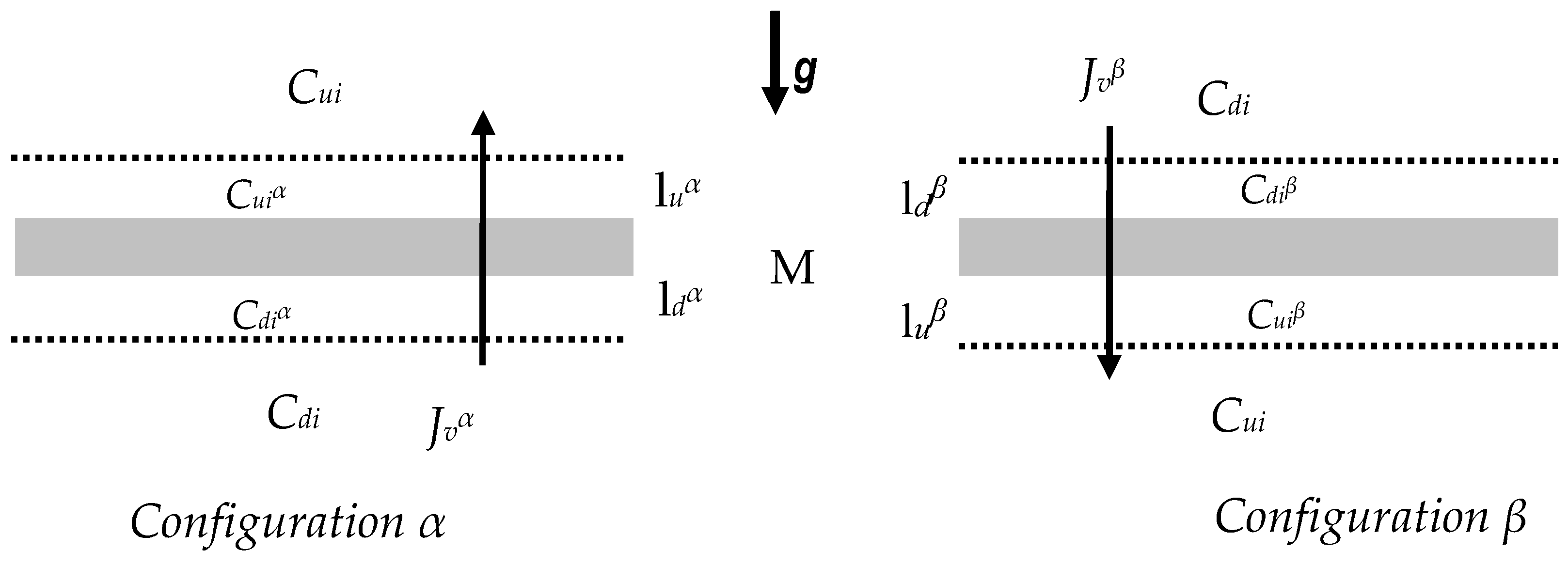
Let us consider membrane transport in a physicochemical cell, shown in Figure 1. In this cell, the membrane (M), arranged in a horizontal plane, at the initial moment (t0 = 0), separated two homogeneous solutions of the same non-electrolytic substance with concentrations Cui i Cdi (Cui > Cdi). If the membrane in question is isotropic, symmetrical, electro-neutral and selective for water and solute, its transport properties are characterized only by the coefficients: hydraulic permeability (Lp), reflection (σi) and permeability of solute (ωi) [21]. For times satisfying the condition t > t0, on both sides of the membrane, the creation of concentration boundary layers begins, which change the concentration field in the areas around the membrane, generating concentration polarization [6,21].
The nature of the concentration field in the areas around the membrane is determined by the density of the solutions separated by the membrane. If the density of the solution with Cui concentration reaches a critical value in relation to the density of the solution with Cdi concentration, then the concentration field changes its nature from diffusive to diffusion - convective. Under the conditions of the diffusion field of concentration, the concentration of the solution, which initially was Cui, decreases to the value or , and the concentration of the solution, which initially was Cd, increases to the value of or (> , > ). In turn, under the conditions of diffusion-convective concentration field, the concentration of the solution that initially amounted to Cui decreases to the value or , and the concentration of the solution that initially amounted to Cdi increases to the value of or ( > , > ). In addition, the conditions > , > , > and > are fullfilled.
Therefore, under the conditions of the diffusion field of concentration, on both sides of the membranes there are concentration boundary layers , , and under conditions of the diffusion-convective field of concentration; concentration boundary layers , , and . The thickness of the layers , , and is much smaller than the layers , , i The thicknesses of layers are denoted by , , i respectively. The concentration boundary layers are treated as pseudomembranes, whose transport properties are determined by the coefficients = = = = 0 and , , and . The volume flux through the complexes /M/ and /M/ will be denoted by and . respectively. Membrane volume transport processes occurring under the conditions of concentration polarization of areas on both sides of the membrane can be described using the first Kedem–Katchalsky equation (for volume flux) [21]. For the homogeneity conditions of diluted electrolyte solutions, this equation can be written as follows.
In turn, for concentration polarization conditions, this equation will take the form [19]
In the above equation, the coefficients of the hydrostatic permeability of the solvent and the reflection of the solute are respectively denoted by Lp and σi. In turn, and are the coefficients of pressure and osmotic concentration polarization, respectively. The symbol fi (1 ≤ fi ≤ 2) means the Vant Hoff coefficient. Expressions (Ph; Pl) = ΔP and RT(Ch; Cl) = Δπ refer to the difference of respectively hydrostatic pressures (Ph, Pl) and osmotic pressures on both sides of the membrane (RT is the product of gas constant and absolute temperature and Ch and Cl; concentration of solutions). The coefficients , , and and , , and are related to the following expressions = (RT)−1, = (RT)−1, = (RT)−1 and = (RT)−1, where , , and is the appropriate diffusion coefficient. The coefficients , , , ωmi, and are related by the equation [22]
where: r = α or β and i = 1 or 2. This equation shows that the value of the coefficient depends on the thickness of the concentration boundary layers i . The process of creating these layers can be followed using a Mach-Zehnder interferometer [7,22,23]. It is also possible, based on interferograms, to determine the time-spatial evolution of the concentration field and to determine the time dependence of the concentration thicknesses of boundary layers [24]. The process of transition from diffusion to convective concentration field can be controlled by the Rayleigh concentration number (RC) [25]. Assuming that = = , = = this number for ternary solutions can be described by the equation [26,27]
where is the gravitational acceleration; ρi is the mass density, νi is the kinematic viscosity of fluid, is the variation of density with the concentration.
Entropy is produced in every membrane system, including the biological one. In the case where the driving forces in the membrane system are the differences in hydrostatic pressure (Δp) and osmotic pressure (Δπk), entropy production () can be described by the equation [10,11]
where: is the flux of i-th solute, is the average solution concentration.
3. Methodology for Measuring the Volume Flux
The study of the volume osmotic flux () was carried out using the measuring set described in the previous paper [18]. This set consisted of two cylindrical measuring vessels (U, D) made of Plexiglas with a volume of 200 cm3 each. Vessel U contained the tested binary or ternary solution, while vessel D had pure water. As binary solutions, aqueous CuSO4 solutions or aqueous ethanol solutions were used. The ternary solutions were ethanol solutions in an aqueous CuSO4 solution or CuSO4 solutions in an aqueous ethanol solution. It should be noted that the density of aqueous ethanol solutions is less than the density of water, and the density of the aqueous solution of CuSO4 is greater than the density of water. In turn, the density of ethanol solutions in aqueous CuSO4 and the density of CuSO4 solutions in aqueous ethanol may be less than, equal to or greater than the density of water.
The U and D vessels were separated by a cellulose acetate membrane called Nephrophan situated in a horizontal plane with an area of S = 3.36 cm2 and transport properties determined, in accordance with Kedem and Katchalsky formalism, by the factors: hydraulic permeability (Lp), reflection (σi) and diffusion permeability (ωi). The Nephrophan membrane is the microporous, highly hydrophilic polymeric filter used in medicine (VEB Filmfabrik, Wolfen, Germany). This membrane is made of cellulose acetate (cello-triacetate (OCO-CH3)n) [28,29]. The electron microscope image of surface and cross-section of these membrane it was presented in ref. [18]. The values of these coefficients for CuSO4 (index 1) and ethanol (index 2), determined in a series of independent experiments, are: Lp = 5 × 10⁻¹² m3N−1s−1, σ1 = 0.17, σ2 = 0.025, ω1 = 0.6 × 10⁻⁹ mol N−1s−1 and ω2 = 1.52 × 10⁻⁹ mol N−1s−1. The U vessel was connected to a graduated pipette (K) positioned in a plane parallel to the membrane plane, which was used to measure the volume increase of the solution (ΔV) filling the vessel. In turn, the vessel D was connected to the water reservoir (N) with adjustable height relative to the pipette K, which served to compensate for the hydrostatic pressure (Δp = 0) present in the measuring set.
Each experiment was performed for the α and β configuration of the membrane system. In the α configuration, the test solution was in the vessel above the membrane, and the water, in the vessel under the membrane. In the β configuration, the order in which the solution and water were positioned relative to the membrane was reversed. The flow tests consisted of measuring the volume increase (ΔV) of the solution in the pipette K at 10 min intervals (Δt). For each configuration, the tests were carried out according to a two-step procedure [15]. In the first stage, the volume flux was determined under mechanical mixing conditions of the solutions separated through the membrane at a speed of 500 rpm. until steady state was achieved. The second stage began with switching off the mechanical stirring of the solutions and consisted in testing the flux until the second steady state was obtained. All the investigations of volume osmotic flows were carried out under isothermal conditions for T = (295 ± 0.5) K. The volume osmotic flux, which is a measure of the volume osmotic flows, was calculated on the basis of the measurement of the change in volume (ΔV) in the pipette K occurring during Δt, through the membrane surface area S, using the formula = ()S−1(Δt)−1 for conditions Δp = 0. The volume osmotic fluxes always occurred from the solution with a lower concentration to the solution with a higher concentration. Investigations of volume osmotic flux in both configurations consisted in determining the , , and for different concentrations and composition of solutions. Each measurement series was repeated three times. The relative error made in determining was not greater than 3%. Based on these characteristics, for the steady state, the characteristics = constant), = constant), = = constant) and = constant) were compiled.
4. Results and Discussion
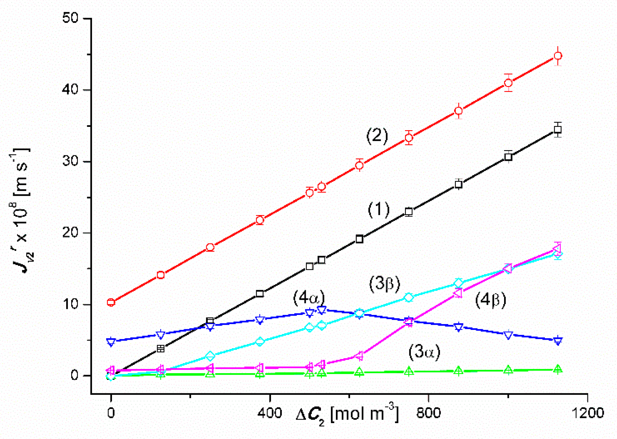
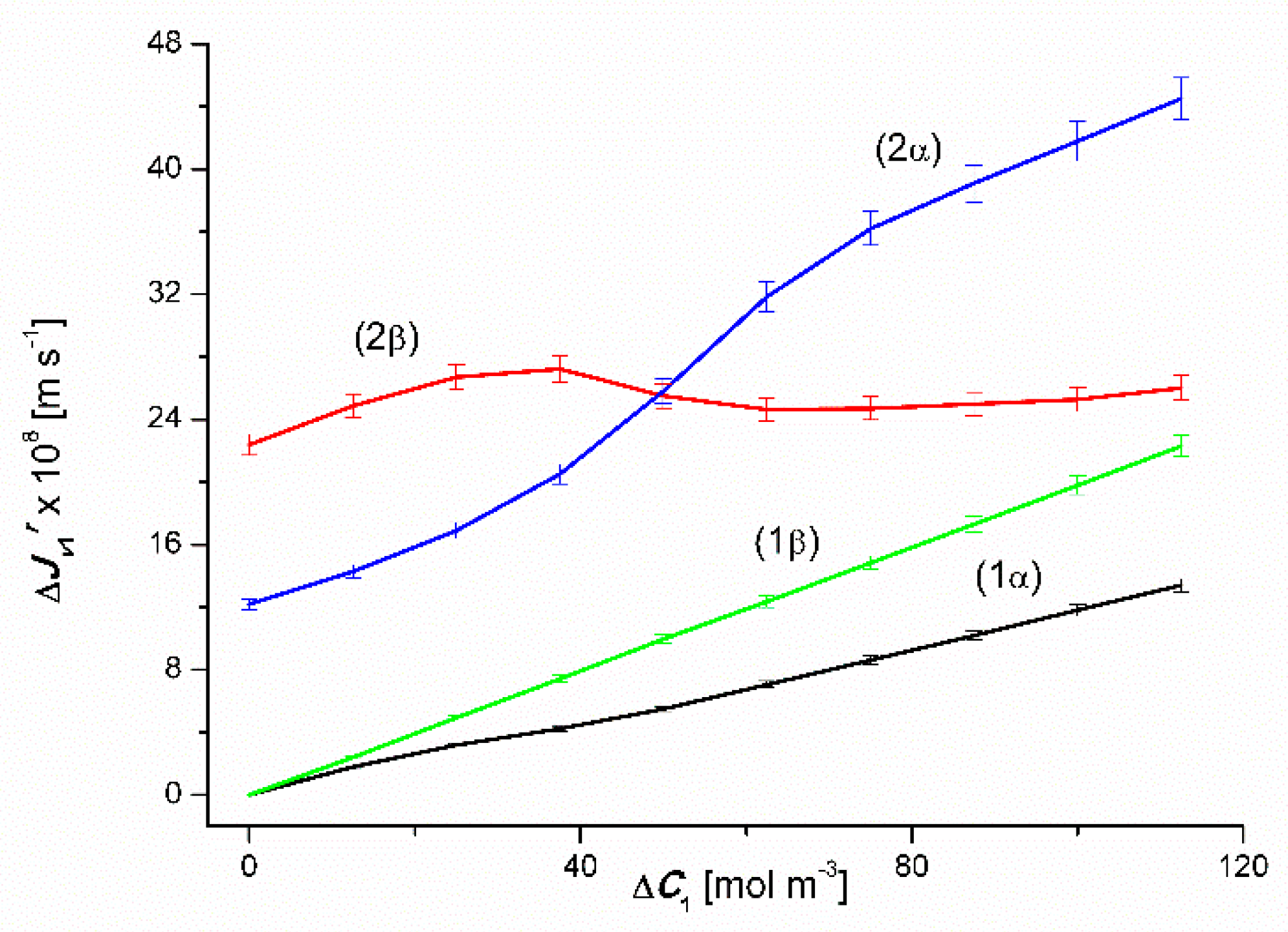
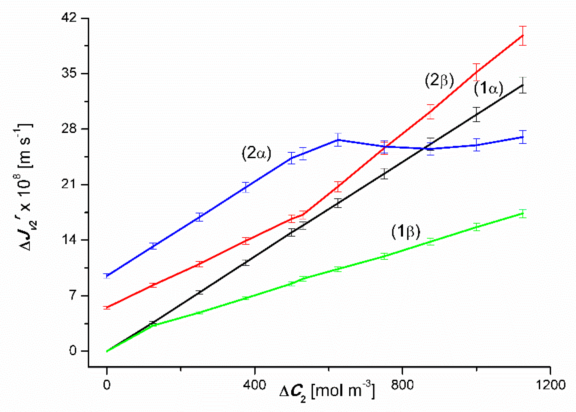
The results of the volume osmotic flux study for the conditions of homogeneity of solutions and conditions of concentration polarization of solutions separated by the membrane are presented in Figure 2 and Figure 3. Figure 2 shows the experimental dependences and = constant) and in Figure 3; experimental dependences = constant) and = constant) for the α (r = α) and β (r = β) configurations of the membrane system, respectively. The dependences shown in Figure 1 and Figure 2 were obtained under mechanical mixing of solutions at a speed of 500 rpm. These dependences for aqueous CuSO4 solutions (Figure 2) and aqueous ethanol solutions (Figure 3) are linear.
Adding a fixed amount of ethanol to aqueous CuSO4 solutions or a fixed amount of CuSO4 to aqueous ethanol solutions causes a parallel shift of the line (1) by a constant and positive volume flux.
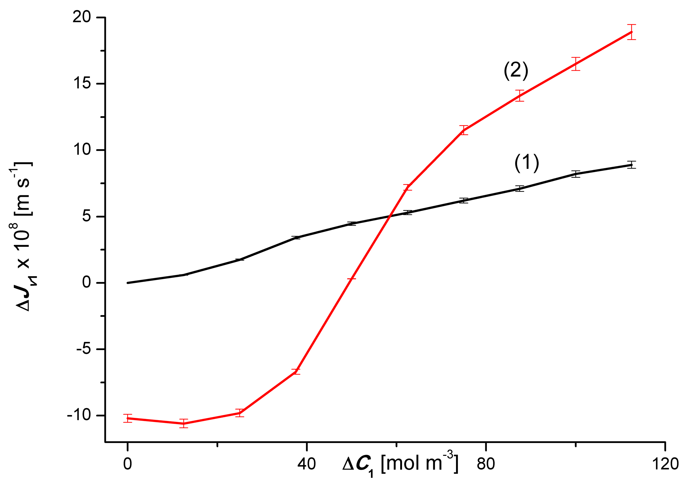
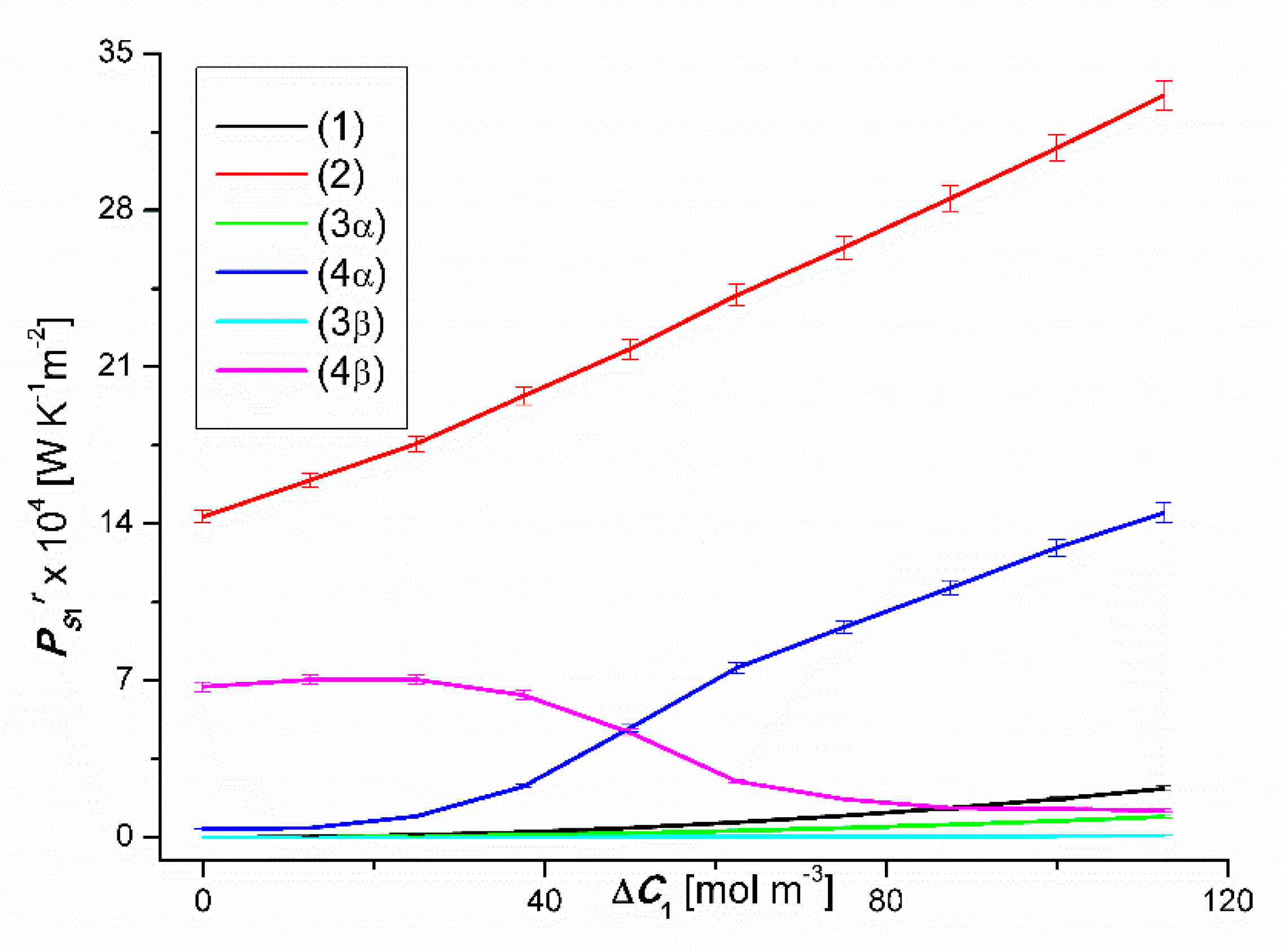
The concentration characteristics of the volume flux for concentration polarization conditions look completely different (after switching off the mechanical stirring of solutions). Graphs 3α and 3β presented in Figure 3 show that an increase in ΔC1 value in binary solutions (water solutions of CuSO4) for ΔC2 = 0, except for the segment 0 < ΔC1 ≤ 50 mol m−3, causes a linear increase in the fluxes and ( > ). In turn, graphs 4α and 4β show that, unlike binary solutions, an increase in ΔC1 in ternary solutions (ΔC2 = 750 mol m−3), causes a non-linear increase in the value of the flux for the α configuration and an initial increase followed by a non-linear decrease in value flux for the β configuration of the membrane system. In the case of the 4α curve shown in Figure 2 (ΔC2 = 750 mol m−3), achieves relatively small values slightly dependent on the value of ΔC1 up to ΔC1 ≤ 50 mol m−3. For ΔC1 > 50 mol m−3 reaches much higher values and strongly dependent on the value of ΔC1. The largest increase in the value of falls within the range of 37.5 mol m−3 < ΔC1 ≤ 62.5 mol m−3. In addition, for ΔC1 > 62.5 mol m−3), increases linearly as the ΔC1 value increases. In turn, the 4β curve shows that initially decreases and for ΔC1 = 18.75 mol m−3 it reaches the minimum value, and then increases non-linearly with an increase in the value of ΔC1 up to ΔC1 = 100 mol m−3. The largest increase in the value of falls within the range of 50 mol m−3 < ΔC1 ≥ 62.5 mol m−3.
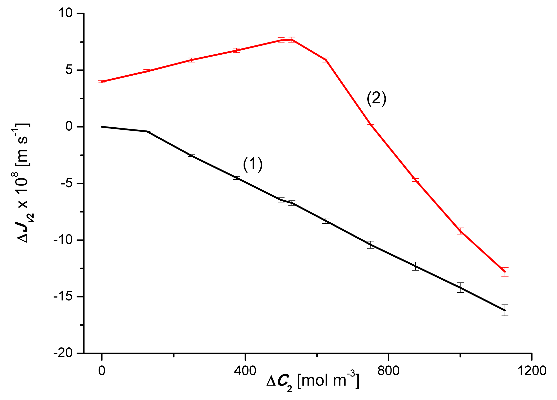
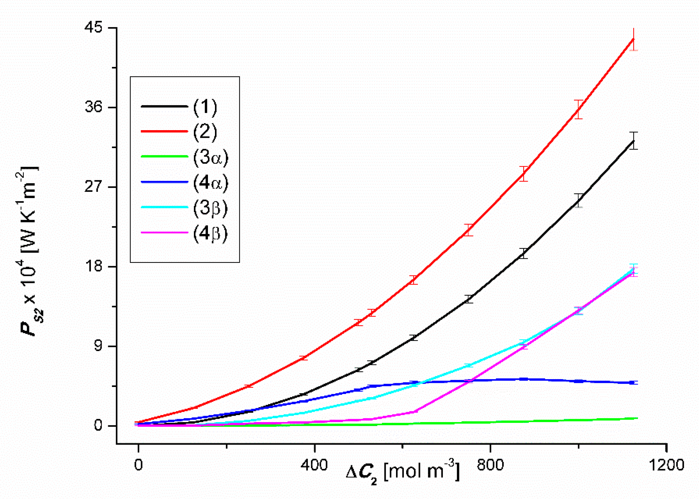
Graphs 3α and 3β presented in Figure 3 show that an increase in the ΔC2 value in binary solutions (aqueous ethanol solutions) for the zero value of the concentration of CuSO4 (ΔC1 = 0), apart from the segment 0 < ΔC2 ≤ 200 mol m−3, causes a linear increase in fluxes and ( < ). In turn, graphs 4α and 4β show that an increase in the value of ΔC2 in ternary solutions (ΔC1 = 50 mol m−3), causes a non-linear increase in the value of the flux for the α configuration and an initial increase followed by a non-linear decrease in the value of the flux for the configuration β of membrane system. In the case of the 4α curve shown in Figure 3 (ΔC1 = 50 mol m−3), increases linearly until the maximum value is = 9.4 × 10⁻⁸ m s−1 for ΔC2 = 540 mol m−3 and then decreases linearly. It should be noted that the increments of the first segment of the 2α graph and the decreases in the value of the second segment of this graph are the same. In turn, the 2β curve shown in this figure shows that the value of is initially independent of ΔC2, and then decreases non-linearly for ΔC2 ≥ 500 mol m−3. The largest increase in the value of occurs in the range of 625 mol m−3 < ΔC2 ≥ 750 mol m−3. To sum up, the creation of concentration boundary layers, which is a consequence of turning off mechanical mixing of solutions, reduces the value of the volume osmotic flux by up to 97%. The appearance of natural convection reduces the reduction by up to 52%.
4.1. The Effect of Concentration Polarization
The measure of the concentration polarization effect () is the equation
where is the volume osmotic flux determined for mechanical stirring conditions of solutions, is the volume osmotic flux determined for concentration polarization conditions, k = 1 or 2 and r = α or β. Figure 4 shows the dependence . This graph shows that for binary solutions > in the whole range of ΔC1. In the case of ternary solutions > , for ΔC1 < 47 mol m−3 and < , for ΔC1 > 47 mol m−3.
Figure 5 shows the dependencies . From this graph it follows that for binary solutions (ΔC1 = 0) > in the whole range of ΔC2. In the case of ternary solutions (ΔC1 = 50 mol m−3) < for ΔC2 < 750 mol m−3 and > , for ΔC1 > 750 mol m−3.
4.2. Convection Effect
The measure of convective effect () is an equation
where is the volume flux determined for concentration polarization conditions of solutions and α configuration of the membrane system, is the volume flux determined for the conditions of concentration polarization of solutions and configuration of the membrane system, k = 1 or 2.
Figure 6 shows the dependence . This graph shows that for binary solutions (ΔC2 = 0) > 0 in the whole range of ΔC1. For ternary solutions (ΔC2 = 750 mol m−3), < 0 for ΔC1 < 47 mol m−3 and > 0, for ΔC1 > 47 mol m−3.
Figure 7 shows the dependence . This graph shows that for binary solutions (ΔC1 = 0), < 0 in the whole range of ΔC2. For ternary solutions (ΔC1 = 50 mol m−3), > 0, for ΔC2 < 750 mol m−3, and < 0, for ΔC2 > 750 mol m−3. It should be noted that the test results presented in Figure 6 and Figure 7 are similar to the results of studies on the gravity-osmotic flux measured in a two-membrane system [14,15]. The membranes in this system were horizontally oriented and separated aqueous solutions of glucose and/or ethanol. The concentrations of these solutions met the condition Cui = Cdi < Cmi (Cui, Cdi; solution concentrations in the external compartments, Cmi; solution concentration in the inter-membrane compartment). The equivalent of such a membrane system is two single-membrane systems connected in parallel.
4.3. The Effect of Asymmetry of the Volume Osmotic Flux
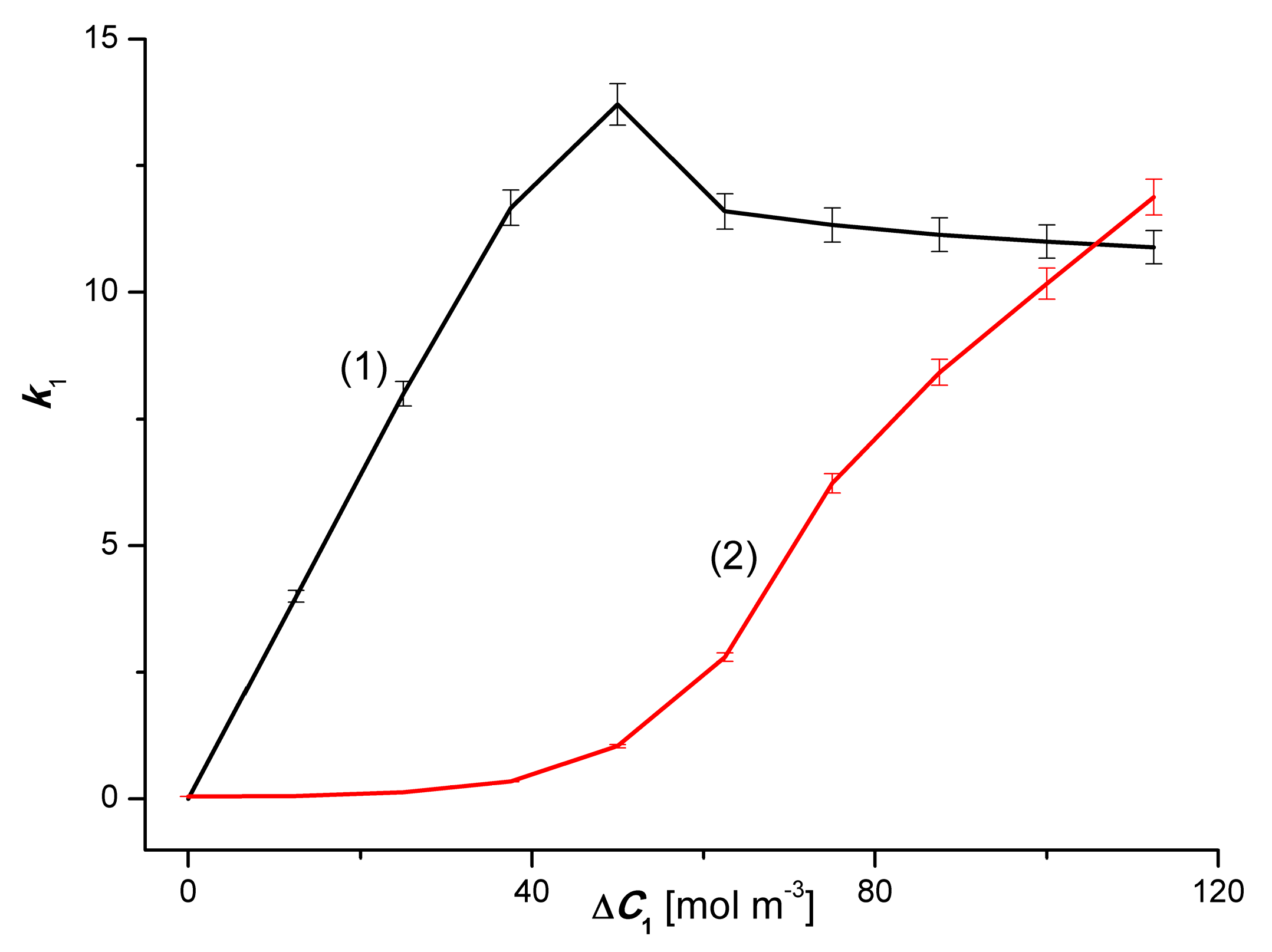
The comparison of the 3α and 3β and 4α and 4β plots presented in Figure 2 and Figure 3 shows the asymmetry of the volume osmotic fluxes, which is the evidence of the osmotic rectifying properties of the membrane system. The measure of this asymmetry is the asymmetry coefficients k1= / and k2 = /. The curves in Figure 8 and Figure 9 show the characteristics of k1 = f(ΔC1, ΔC2 = constant) and k2 = f(ΔC2, ΔC1 = constant). Graphs 1 in Figure 8 and Figure 9 illustrate the dependences k1 = f(ΔC1, ΔC2 = 0) and k2 = f(ΔC2, ΔC1 = 0). respectively. In turn, graphs 2 presented in these graphs illustrate the k1 = f(ΔC1, ΔC2 = 750 mol m−3) and k2 = f(ΔC2, ΔC1 = 50 mol m−3). The values of k1 and k2 coefficients, different from unity, indicate that the tested membrane system has rectifying properties, which are manifested as the asymmetry of the volume osmotic flux.
4.4. The Effect of Amplification the Volume Osmotic Flux
The measure of the amplification effect of the osmotic volume flux is the amplification coefficient, the definition of which is the equation
where is the volume flux increase for ternary solutions, is the volume flux increase for ternary solutions, k = 1 or 2 and r = α or β.
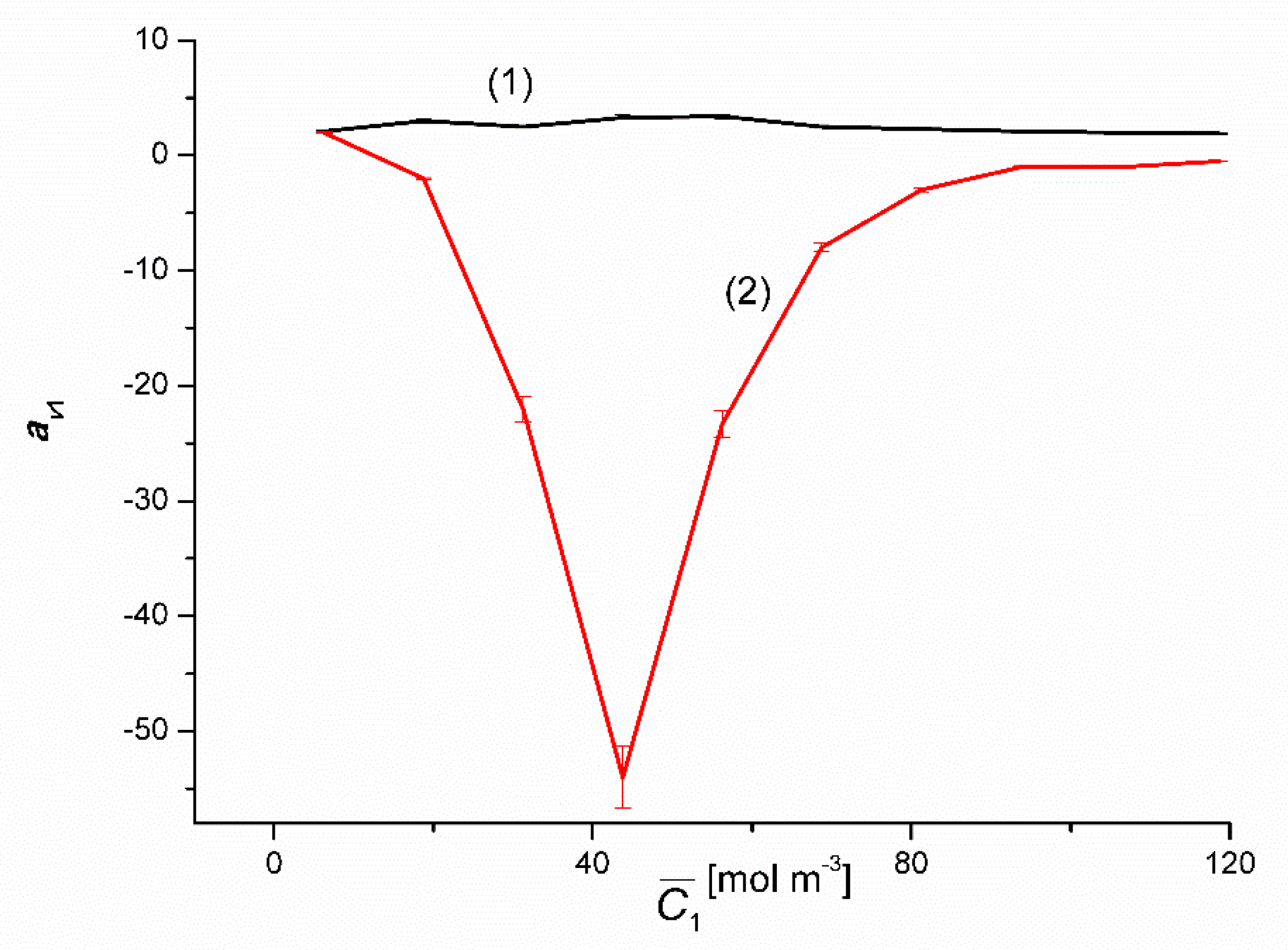
Figure 10 and Figure 11 show the dependencies , where = 0.5(Cj + Cj+1), j = 1, 2, …). Figure 10 shows that for binary solutions (ΔC2 = 0) > 0 in the whole range and takes values from = 2.1 to = 3.3. In the case of ternary solutions (ΔC2 = 750 mol m−3), the dependence is nonlinear, with a clearly marked minimum, and the coefficient is negative. The minimum of this dependence has the coordinates = 43.75 mol m−3 and = −54.
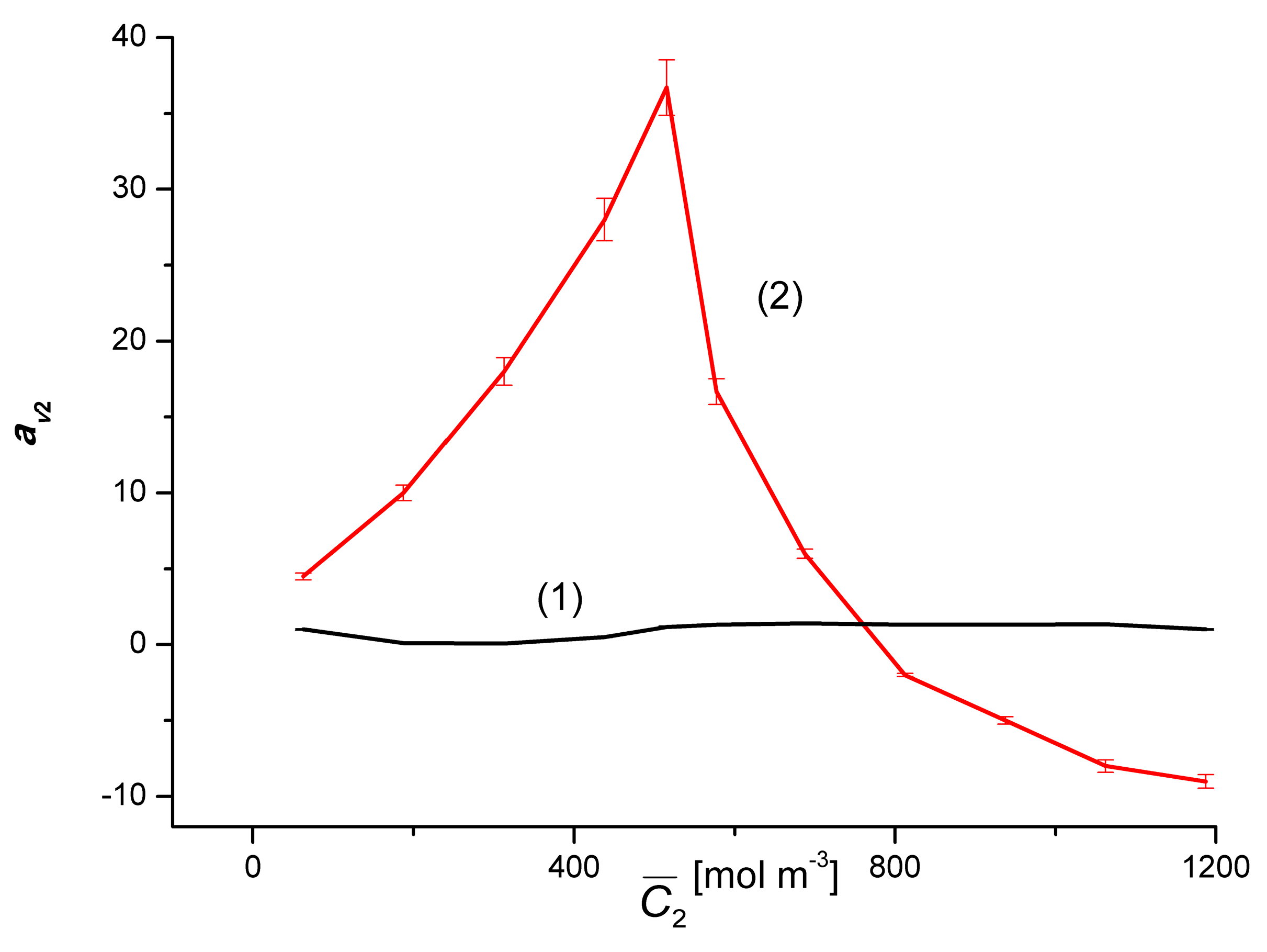
In turn, Figure 11 shows that for binary solutions (ΔC1 = 0), > 0 in the whole range and takes values from = 0.5 to = 1.4. In the case of ternary solutions (ΔC1 = 50 mol m−3), the dependence is non-linear, with the maximum clearly indicated, and the coefficient assumes positive values for < 760 mol m−3 and negative for < 760 mol m−3. The maximum of this dependence has the coordinates = 515.75 mol m−3 and = 36.7. Rectifying properties along with amplification properties and oscillation generation belong to the group of regulatory phenomena [19].
4.5. Evaluation of Osmotic Entropy Production
The osmotic entropy production () will be calculated using Equation (5), omitting the term and assuming that Δp = 0 and i = 1, 2. With such assumptions the Equation (5) will take the form
This equation shows that is directly proportional to, among others, . Taking into account the results of presented in Figure 2 and Figure 3 in the above equation, the relationships and , (r = α, β). The results of the calculations are presented in Figure 12 and Figure 13. These figures show that for the same values i , both and follow the changes in the values of or . Under the conditions of homogeneity of the solutions and they increase with the increase of the values of and , respectively. On the other hand, under the conditions of concentration polarization, the values and increase when free convection appears in the membrane system and decreases when convection disappears. Due to the fact that concentration polarization reduces and , it also reduces and .
Equations (2)–(4) will be used to interpret the results of osmotic volume flux tests for concentration polarization conditions and presented in Figure 2 and Figure 3. For this purpose, Equation (2), for pu; pd = 0, will be transformed into the form
Having Equation (3) in the above equation, we get
Assuming that = = , = = and f2 = 1, the equation can be written in a simplified form, namely
Based on Equation (10), the dependencies = constant), = constant), = 50 mol m−3) and = 50 mol m−3) were calculated. The following data was used for RC calculations: D1 = 0.73 × 10⁻⁹ m2s−1, D2 = 1.37 × 10⁻⁹ m2s−1, R = 8.31 J mol−1K−1, T = 295 K, Lp = 5 × 10⁻¹² m3N−1s−1, σ1 = 0.17, σ2 = 0.025, ωm1 = 0.6 × 10⁻⁹ mol N−1s−1 and ωm2 = 1.52 × 10⁻⁹ mol N−1s−1, f1 = 2 and f2 = 1. The results of the calculations are illustrated in Figure 14 and Figure 15.
The curves 1α and 1β presented in Figure 14 illustrate the dependencies = 0) and = 0), while the curves 2α and 2β ̶ dependencies = 750 mol m−3) and = 750 mol m−3). From the course of the 1α and 1β curves, it can be seen that the values of decrease and ̶ increase non-linearly. For ΔC1 = 5.1 mol m−3 = = 1.02 × 10⁻³ m, which means that the value of is independent of the configuration of the membrane system and thus also of the dependence between the gravity vector and the density gradient of binary solutions separated through the membrane. For ΔC1 ≥ 25 mol m−3, the value of is approximately constant and amounts to about = 0.9 × 10⁻³ m and for ΔC1 ≥ 50 mol m−3 = 12.7 × 10⁻³ m = constant, and therefore < . This means that for ΔC1 ≥ 25 mol m−3 and the α configuration of the membrane system, convection fluxes generated in the membrane areas destroy the concentration boundary layers, increasing the volume flux through the membrane.
For the 2α and 2β curves in this figure, the values of initially increase linearly and then, after reaching the maximum value = 9.9 × 10⁻³ m for ΔC1 = 6.25 mol m−3 decrease non-linearly. In turn, the values of increase non-linearly. For ΔC1 = 50 mol m−3 = = 1.02 × 10⁻³ m, which means that the value of is independent of the configuration of the membrane system and thus also of the dependence between the gravity vector and the density gradient of ternary solutions separated through the membrane. Comparing graphs 2α and 2β, it can be seen that for ΔC1 < 50 mol m−3, < while for ΔC1 > 50 mol m−3, > . This means that for ΔC1 > 50 mol m−3 and the β configuration of the membrane system (curve 2β), and for ΔC1 < 50 mol m−3 and the configuration of the membrane system (curve 2α), the convection fluxes generated in the membrane areas cause concentration destruction of boundary layers, increasing the volume flow through the membrane.
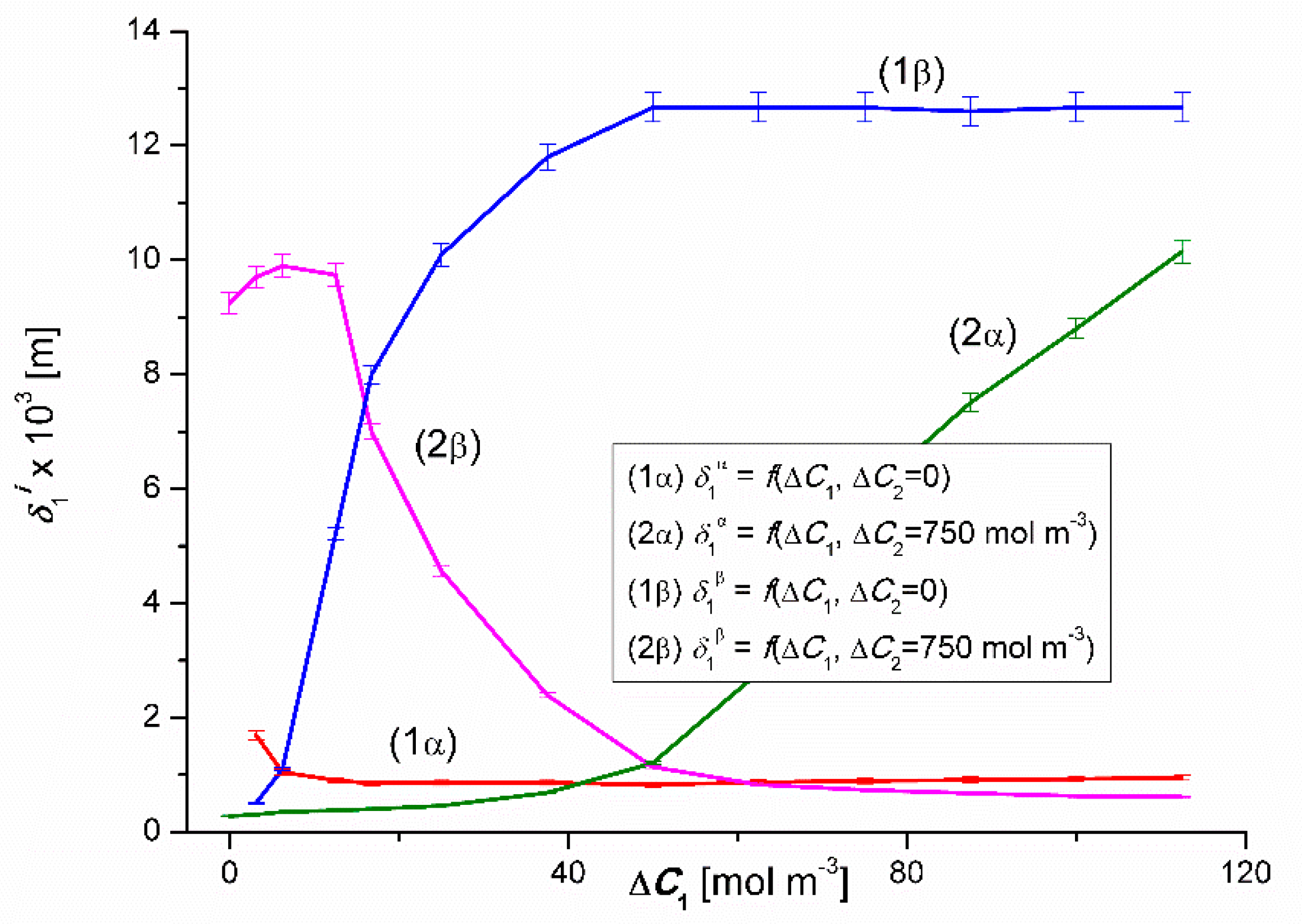
The curves 1α and 1β presented in Figure 15 illustrate the dependencies =0) and = 0), while the curves 2α and 2β ̶ dependencies 50 mol m−3) and = 50 mol m−3). From the course of the 1α and 1β curves, it can be seen that the values of initially increase non-linearly and ̶ decrease non-linearly. For ΔC2 = 50 mol m−3, = = 0.94 × 10⁻³ m, which means that the value of is independent of the configuration of the membrane system and thus also of the dependence between the gravity vector and the density gradient of binary solutions separated through the membrane. For ΔC2 ≥ 375 mol m−3 = 6.8 × 10⁻³ m = const. and for ΔC2 ≥ 375 mol m−3 = 0.2 × 10⁻³ m = const., and therefore > . This means that for ΔC2 ≥ 375 mol m−3 in the β configuration of the membrane system, convection fluxes generated in the membrane regions destroy the concentration boundary layers, increasing the volume flow through the membrane.
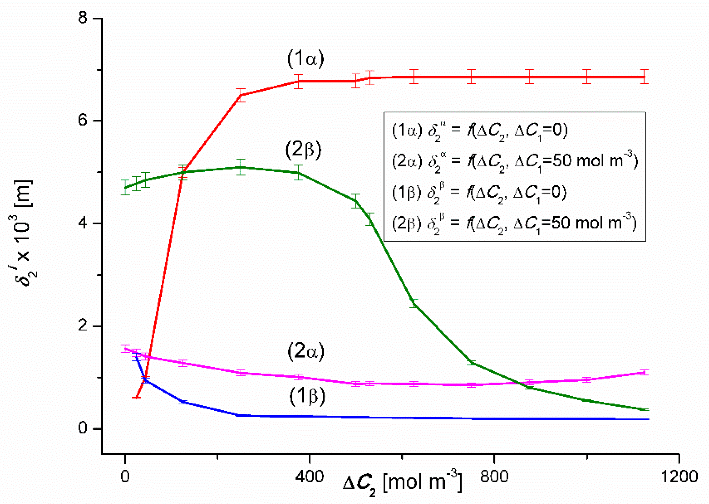
In the case of the 2α and 2β curves in this figure, the values of initially increase and then, after reaching the maximum value = 5.1 × 10⁻³ m for ΔC2 = 250 mol m−3 decrease non-linearly. In turn, the values of change non-linearly. For ΔC2 = 850 mol m−3 = = 0.92 ×10⁻³ m, which means that the value of is independent of the configuration of the membrane system and thus also of the dependence between the gravity vector and the density gradient of ternary solutions separated through the membrane. Comparing graphs 2α and 2β, it can be seen that for ΔC2 < 840 mol m−3 < , while for ΔC2 > 840 mol m−3, > . This means that for ΔC1 > 840 mol m−3 and the β configuration of the membrane system (graph 2β), and for ΔC1 < 840 mol m−3 and the α configuration of the membrane system (graph 2 α), the convection fluxes generated in the membrane areas cause concentration destruction of the boundary layers, increasing the volume flux through the membrane.
As already mentioned, the Rayleigh concentration number (), which is the parameter controlling the transition from non-convective to convective state can be expressed using Equation (4). We assume that at the point where = = , (i = 1, 2) the concentration number meets the condition = = . Calculations will be made for the following data D1 = 0.73 × 10⁻⁹ m2s−1, D2 = 1.37 × 10⁻⁹ m2s−1, ω1 = 0.6 × 10⁻⁹ mol N−1s−1, ω2 = 1.52 × 10⁻⁹ mol N−1s−1, ρ0 = 998 kg m−3, ν0 = 1.012 × 10⁻⁶ m2s−1, (∂ρ/∂C1)bin. = 0.06 kg mol−1 (for ΔC2 = 0), (∂ρ/∂C1)ter. = 0.05 kg mol−1 (for ΔC2 = 750 mol m−3), (∂ρ/∂C2)bin. = −0.0095 kg mol−1 (for ΔC1 = 0) and (∂ρ/∂C2)ter. = −0.0035 kg mol−1 (for ΔC1 = 50 mol m−3). It should be noted that ∂ρ/∂Ci (i = 1, 2) is added for solutions whose density increases with increasing concentration and negative ̶ when the density of solutions decreases with increasing concentration. Therefore, the indication is determined by the indication ∂ρ/∂Ci. For calculations the values of = = (i = 1, 2) will be used, taken from the curves presented in Figure 14 and Figure 15. Graphs 1α and 1β intersect at a point with coordinates ΔC1 = 5.1 mol m−3 and = = 1.02 × 10⁻³ m. Taking the relevant data into Equation (4) gives = 1737.89. In turn, the curves 2α and 2β presented in Figure 14 intersect at a point with coordinates ΔC1 = 50 mol m−3 and = = 1.02 × 10⁻³ m. Therefore, taking into account relevant data in Equation (4) gives = 1335.69. Figure 15 shows that the diagrams 1α and 1β intersect at a point with the coordinates ΔC2 = 50 mol m−3 = = 0.92 × 10⁻³ m. Therefore, taking into account the relevant data in Equation (4) gives = −1169.79. Figure 15 also shows that the graphs 2α and 2β intersect at a point with the coordinates ΔC2 = 850 mol m−3 = = 0.92 ×10⁻³ m. Therefore, taking into account relevant data in Equation (4) we get = −1408.68.
Graphs 1α and 1β show that for < and > non-convective state in both configurations of the membrane system is being dealt with. > in the α configuration (graphs 1α and 2α) a convective state is obtained and in the β configuration (graphs 1β and 2β) ̶ the non-convective state. On the other hand, for < in the α configuration (graphs 1α and 2α) a non-convective state is obtained, and for the β configuration (graphs 1β and 2β); the convective state. Therefore, the authors have shown that the concentration Rayleigh number () is a parameter controlling the transition from non-convective to convective state. This number also acts as a switch between two convective states (with a higher value) and non-convective states (with a lower value). The operation of this switch indicates the regulatory role of earthly gravity in relation to membrane transport.
Investigations on membrane transport are one of the most forward-looking directions in biotechnology, biomedical engineering and environmental protection and engineering, especially in water treatment and purification. Moreover, in recent years the research on integrated membrane processes has also been carried out [30]. The research results presented in the paper may also be relevant for nature-inspired chemical engineering (NICE) [31].
5. Conclusions
In this article, the authors presented the results of studies on the impact of the concentration of individual solution components and the configuration of the membrane system on the value of the volume osmotic flux in a single-membrane system, in which the polymer membrane was positioned in a horizontal plane and separated water and a ternary solution consisting of water, ethanol and/or CuSO4. From the studies it results, that for conditions of concentration polarization and binary solutions is a linear and for ternary solutions a non-linear function of the solution concentration differences. In addition, depends on the configuration of the membrane system. For mechanically stirred solutions, is independent of the membrane system configuration and is a linear function of the difference in solution concentrations. The effects of concentration polarization, convective polarization, asymmetry and amplification of the volume osmotic flux calculated on the basis of measurements are a consequence of the concentration polarization of solutions adjacent to the membrane. The effects of concentration polarization and convective polarization for binary solutions are linear and for ternary ones a non-linear function of the concentration difference. The measures of asymmetry and amplification of the volume osmotic flux (which are a consequence of concentration polarization) are the corresponding asymmetry coefficients k1 and k2 and the amplification coefficients av1 and av2. The k1 coefficient for both binary and ternary solutions is a non-linear function of the difference in concentration of CuSO4. In turn, the value of the coefficient k2 for binary solutions is independent of the concentration and for ternary solutions; it is a non-linear function of the difference in ethanol concentration. For binary solutions, the values of av1 and av2 coefficients are constant and positive. In turn, for ternary solutions, these coefficients are a non-linear function of the respective concentration differences and assume both positive and negative values.
It has been shown that entropy production occurs in the single-membrane system study, which is a consequence of two thermodynamic forces (one variable and the other constant) and the generation of an osmotic flux. It has been shown, that the factor , by the thickness of the concentration boundary layer (, can be associated with the Rayleigh concentration number (), i.e., the parameter controlling the transition from non-convection (diffusion) to convective concentration field. Four different concentration Rayleigh number, which differ in values and signs were obtained.
The signs is conditioned by the relationship between the gravity vector and the solution density gradient. It has been shown that this number also acts as a switch between two states of the concentration field: convective (with a higher value) and non-convective (with a lower value). The operation of this switch indicates the regulatory role of earthly gravity in relation to membrane transport.
Author Contributions
Conceptualization, K.M.B. and A.Ś.: methodology, K.M.B. and A.Ś.: calculation and investigation: K.M.B., A.Ś.; writing; original draft preparation, K.M.B., A.Ś. and W.M.B.; writing; review and editing K.M.B., A.Ś. and W.M.B. All authors have read and agreed to the published version of the manuscript.
Funding
This research received no external funding.
Acknowledgments
We would like to thank our astoundingly supportive research team and for those who have touched our science paths.
Conflicts of Interest
The authors declare no conflict of interest.
References
- Lipton, B. The Biology of Belief: Unleashing the Power of Consciousness; Hay House: Carlsbad, CA, USA, 2018; ISBN 10: 1401923127. [Google Scholar]
- Baker, R. Membrane Technology and Application; John Wiley & Sons: New York, NY, USA, 2012; ISBN 978-0-470-74372-0. [Google Scholar]
- Nunes, S.P.; Culfaz-Emecen, P.Z.; Ramon, G.Z.; Visser, T.; Koops, G.H.; Jin, W.; Ulbricht, M. Thinking the future of membranes: Perspectives for advanced and new membrane materials and manufacturing processes. J. Membr. Sci. 2020, 598, 117761. [Google Scholar] [CrossRef]
- Nguyen, T.P.N.; Jun, B.M.; Hwa Lee, J.; Kwon, Y.-M. Comparison of integrally asymmetric and thin film composite structures for a desirable fashion of forward osmosis membranes. J. Membr. Sci. 2015, 495, 457–470. [Google Scholar] [CrossRef]
- Nga Nguyen, T.P.; Byung-Moon, N.; Kwon, Y.N. The chlorination mechanism of integrally asymmetric cellulose triacetate (CTA)-based and thin film composite polyamide-based forward osmosis membrane. J. Membr. Sci. 2017, 523, 111–121. [Google Scholar] [CrossRef]
- Barry, P.H.; Diamond, J.M. Effects of unstirred layers on membrane phenomena. Physiol. Rev. 1984, 64, 763–872. [Google Scholar] [CrossRef]
- Dworecki, K.; Ślęzak, A.; Ornal-Wąsik, B.; Wąsik, S. Effect of hydrodynamic instabilities on solute transport in membrane system. J. Membr. Sci. 2005, 265, 94–100. [Google Scholar] [CrossRef]
- Nikonenko, V.V.; Kovalenko, A.V.; Urtenov, M.K.; Pismenskaya, N.D.; Han, J.; Sistet, P.; Pourcelly, G. Desalination at overlimitinng currents: state-of-theart and perspectives. Desalination 2014, 342, 85–106. [Google Scholar] [CrossRef]
- Batko, K.M.; Ślęzak-Prochazka, I.; Ślęzak, A. Network hybrid form of the Kedem-Katchalsky equations for non-homogenous binary non-electrolyte solutions: Evaluation of Pij* Peusner’s tensor coefficients. Transp. Porous Med. 2015, 106, 1–20. [Google Scholar] [CrossRef] [Green Version]
- Ślęzak, A.; Ślęzak-Prochazka, I.; Grzegorczyn, S.; Jasik-Ślęzak, J. Evaluation of S-Entropy production in a single-membrane system in concentration polarization conditions. Trans. Porous Med. 2017, 116, 941–957. [Google Scholar] [CrossRef]
- Dermirel, Y. Nonequilibrium Thermodynamics: Transport and Rate Processes in Physical, Chemical and Biological Systems; Elsevier: Amsterdam, The Netherlands, 2007; pp. 275–540. ISBN 978-0-444-53079-0. [Google Scholar]
- Delmotte, M.; Chanu, J. Non-equilibrium thermodynamics and membrane potential measurement in biology. In Topics Bioelectrochemistry and Bioenergetics; Millazzo, G., Ed.; John Wiley Publish & Sons: Chichester, UK, 1979; pp. 307–359. [Google Scholar]
- Przestalski, S.; Kargol, M. Graviosmotic volume flow through membrane systems. Stud. Biophys. 1972, 34, 7–14. [Google Scholar]
- Kargol, M.; Dworecki, K.; Przestalski, S. Graviosmotic flow amplification effects in a series membrane system. Stud. Biophys. 1979, 76, 137–144. [Google Scholar]
- Kargol, M. The graviosmotic hypothesis of xylem transport of water in plants. Gen. Physiol. Biophys. 1992, 11, 469–487. [Google Scholar] [PubMed]
- Ślęzak, A.; Dworecki, K.; Anderson, J.A. Gravitational effects on transmembrane flux: the Rayleigh-Taylor convective instability. J. Membr. Sci. 1985, 23, 71–81. [Google Scholar] [CrossRef]
- Ślęzak, A. Irreversible thermodynamic model equations of the transport across a horizontally mounted membrane. Biophys. Chem. 1989, 34, 91–102. [Google Scholar] [CrossRef]
- Ślęzak, A.; Grzegorczyn, S.; Jasik-Ślęzak, J.; Michalska-Małecka, K. Natural convection as an asymmetrical factor of the transport through porous membrane. Transp. Porous Media 2010, 84, 685–698. [Google Scholar] [CrossRef]
- Batko, K.M.; Ślęzak-Prochazka, I.; Grzegorczyn, S.; Ślęzak, A. Membrane transport in concentration polarization conditions: network thermodynamics model equations. J. Porous. Media 2014, 17, 573–586. [Google Scholar] [CrossRef]
- Ślęzak, A.; Jasik-Ślęzak, J.; Wąsik, J.; Sieroń, A.; Pilis, W. Volume osmotic flows of non-homogeneous electrolyte solutions through horizontally mounted membrane. Gen. Physiol. Biophys. 2001, 21, 115–146. [Google Scholar]
- Katchalsky, A.; Curran, P.F. Nonequilibrium Thermodynamics in Biophysics; Harvard University Press: Cambridge, MA, USA, 1965; ISBN 9780674494121. [Google Scholar]
- Ślęzak, A.; Dworecki, K.; Ślęzak, I.H.; Wąsik, S. Permeability coefficient model equations of the complex: Membrane-concentration boundary layers for ternary nonelectrolyte solutions. J. Membr. Sci. 2005, 267, 50–57. [Google Scholar] [CrossRef]
- Dworecki, K.; Wąsik, S.; Ślęzak, A. Temporal and spatial structure of the concentration boundary layers In membrane system. Physica A 2003, 326, 360–369. [Google Scholar] [CrossRef]
- Ślęzak, A.; Jasik-Ślęzak, J.; Grzegorczyn, S.; Ślęzak-Prochazka, I. Nonlinear effects in osmotic volume flows of electrolyte solutions through double-membrane system. Transp. Porous Med. 2012, 92, 337–356. [Google Scholar] [CrossRef]
- Lebon, G.; Jou, D.; Casas-Vasquez, J. Understanding Non-Equilibrium Thermodynamics. Foundations, Applications, Frontiers; Springer: Berlin/Heidelberg, Germany, 2008. [Google Scholar] [CrossRef] [Green Version]
- Jasik-Ślęzak, J.; Olszówka, K.M.; Ślęzak, A. Estimation of thickness of concentration boundary layers by osmotic volume flux determination. Gen. Physiol. Biophys. 2011, 30, 186–195. [Google Scholar] [CrossRef]
- Ślęzak, A.; Dworecki, K.; Jasik-Ślęzak, J.; Wąsik, J. Method to determine the critical concentration Rayleigh number in isothermal passive membrane transport processes. Desalination 2004, 168, 397–412. [Google Scholar] [CrossRef]
- Klinkman, H.; Holtz, M.; Willgerodt, W.; Wilke, G.; Schoenfelder, D. “Nephrophan”— eine neue dialysemembran. Zeits. Urolog. Nephrol. 1969, 62, 285–294. [Google Scholar]
- Richter, T.; Keipert, S. In vito permeation studies comparing bovine nasal mucosa, porcine cornea and art.ificial membrane: Androdtenedione in microemulsions and their components. Europ. J. Pharmac. Biopharmac. 2004, 58, 137–143. [Google Scholar] [CrossRef] [PubMed]
- Korus, I.; Rajca, M. Membranes and membrane processes in environmental protection. In Proceedings of the MEMPEP 2018, 12th Scientific Conference, Zakopane, Poland, 13–16 June 2018; Silesia Technical University Press: Gliwice, Poland, 2018; pp. 120–121. [Google Scholar]
- Gerbaud, V.; Shcherbakova, N.; Da Cunha, S. A nonequilibrium thermodynamics perspective on nature-inspired chemical engineering processes. Chem. Eng. Res. Des. 2020, 154, 316–330. [Google Scholar] [CrossRef]
Figure 1.
Single membrane system: M = membrane; Cui and Cdi (Cui > Cdi, k = 1 or 2) = solution concentrations; , Jviβ (k = 1 or 2) = volume flux for the α and β configuration of the membrane system, respectively.
Figure 1.
Single membrane system: M = membrane; Cui and Cdi (Cui > Cdi, k = 1 or 2) = solution concentrations; , Jviβ (k = 1 or 2) = volume flux for the α and β configuration of the membrane system, respectively.

Figure 2.
Graphic illustration of the experimental dependence , (r = α, β) for CuSO4 solutions in aqueous ethanol and the α and β configurations of the membrane system. Graphs 1, 3α and 3β were obtained for ΔC2 = 0, graphs 2, 4α and 4β; for ΔC2 = 750 mol m−3.
Figure 2.
Graphic illustration of the experimental dependence , (r = α, β) for CuSO4 solutions in aqueous ethanol and the α and β configurations of the membrane system. Graphs 1, 3α and 3β were obtained for ΔC2 = 0, graphs 2, 4α and 4β; for ΔC2 = 750 mol m−3.

Figure 3.
Graphic illustration of the experimental dependence , (r = α, β) for ethanol solutions in aqueous CuSO4 and the α and β configurations of the membrane system. Graphs 1, 3α and 3β were obtained for ΔC1 = 0, graphs 2, 4α and 4β; for ΔC1 = 50 mol m−3.
Figure 3.
Graphic illustration of the experimental dependence , (r = α, β) for ethanol solutions in aqueous CuSO4 and the α and β configurations of the membrane system. Graphs 1, 3α and 3β were obtained for ΔC1 = 0, graphs 2, 4α and 4β; for ΔC1 = 50 mol m−3.

Figure 4.
Graphic illustration of the dependence , (r = α, β) for CuSO4 solutions in aqueous ethanol and the α and β configurations of the membrane system. Graphs 1α and 1β were obtained for ΔC2 = 0, graphs 2α and 2β; for ΔC2 = 750 mol m−3.
Figure 4.
Graphic illustration of the dependence , (r = α, β) for CuSO4 solutions in aqueous ethanol and the α and β configurations of the membrane system. Graphs 1α and 1β were obtained for ΔC2 = 0, graphs 2α and 2β; for ΔC2 = 750 mol m−3.

Figure 5.
Graphic illustration of the dependence , (r = α, β) for ethanol solutions in the aqueous solution of CuSO4 and α and β configurations of the membrane system. Graphs 1α and 1β were obtained for ΔC1 = 0, graphs 2α and 2β; for ΔC1 = 50 mol m−3.
Figure 5.
Graphic illustration of the dependence , (r = α, β) for ethanol solutions in the aqueous solution of CuSO4 and α and β configurations of the membrane system. Graphs 1α and 1β were obtained for ΔC1 = 0, graphs 2α and 2β; for ΔC1 = 50 mol m−3.

Figure 6.
Graphic illustration of the dependence , (r = α, β) for CuSO4 solutions in aqueous ethanol and the α and β configurations of the membrane system. Graph 1 was obtained for ΔC2 = 0, graph 2; ΔC2 = 750 mol m−3.
Figure 6.
Graphic illustration of the dependence , (r = α, β) for CuSO4 solutions in aqueous ethanol and the α and β configurations of the membrane system. Graph 1 was obtained for ΔC2 = 0, graph 2; ΔC2 = 750 mol m−3.

Figure 7.
Graphic illustration of the dependence , (r = α, β) for ethanol solutions in aqueous CuSO4 solution and α and β configurations of the membrane system. Graph 1 was obtained for ΔC1 = 0, graph 2; for ΔC1 = 50 mol m−3.
Figure 7.
Graphic illustration of the dependence , (r = α, β) for ethanol solutions in aqueous CuSO4 solution and α and β configurations of the membrane system. Graph 1 was obtained for ΔC1 = 0, graph 2; for ΔC1 = 50 mol m−3.

Figure 8.
Graphic illustration of the dependence k1 = f(ΔC1, ΔC2 = constant). For solutions of CuSO4 in aqueous ethanol. Graphs 1 and 2 were obtained for ΔC2 = 0 and ΔC2 = 750 mol m−3, respectively.
Figure 8.
Graphic illustration of the dependence k1 = f(ΔC1, ΔC2 = constant). For solutions of CuSO4 in aqueous ethanol. Graphs 1 and 2 were obtained for ΔC2 = 0 and ΔC2 = 750 mol m−3, respectively.

Figure 9.
Graphic illustration of the dependence k2 = f(ΔC2, ΔC1 = constant) for ethanol solutions in aqueous CuSO4. Graphs 1 and 2 were obtained for ΔC1 = 0 and ΔC1 = 50 mol m−3, respectively.
Figure 9.
Graphic illustration of the dependence k2 = f(ΔC2, ΔC1 = constant) for ethanol solutions in aqueous CuSO4. Graphs 1 and 2 were obtained for ΔC1 = 0 and ΔC1 = 50 mol m−3, respectively.

Figure 10.
Graphic illustration of the dependence = f(, ΔC2 = constant) for solutions of CuSO4 in aqueous ethanol. Graphs 1 and 2 were obtained for ΔC2 = 0 and ΔC2 = 750 mol m−3, respectively.
Figure 10.
Graphic illustration of the dependence = f(, ΔC2 = constant) for solutions of CuSO4 in aqueous ethanol. Graphs 1 and 2 were obtained for ΔC2 = 0 and ΔC2 = 750 mol m−3, respectively.

Figure 11.
Graphic illustration of the relationship = f(, ΔC1 = constant) for solutions of ethanol in an aqueous solution of CuSO4. Graphs 1 and 2 were obtained for ΔC1 = 0 and ΔC1 = 50 mol m−3, respectively.
Figure 11.
Graphic illustration of the relationship = f(, ΔC1 = constant) for solutions of ethanol in an aqueous solution of CuSO4. Graphs 1 and 2 were obtained for ΔC1 = 0 and ΔC1 = 50 mol m−3, respectively.

Figure 12.
Graphic illustration of the dependencies , (r = α, β) for CuSO4 solutions in aqueous ethanol and the α and β configurations of the membrane system. Graphs 1, 3α and 3β were obtained for ΔC2 = 0, graphs 2, 4α and 4β; for ΔC2 = 750 mol m−3.
Figure 12.
Graphic illustration of the dependencies , (r = α, β) for CuSO4 solutions in aqueous ethanol and the α and β configurations of the membrane system. Graphs 1, 3α and 3β were obtained for ΔC2 = 0, graphs 2, 4α and 4β; for ΔC2 = 750 mol m−3.

Figure 13.
Graphic illustration of the dependencies , (r = α, β) for ethanol solutions in aqueous CuSO4 and the α and β configurations of the membrane system. Graphs 1, 3α and 3β were obtained for ΔC1 = 0, graphs 2, 4α i 4β; for ΔC1 = 50 mol m−3.
Figure 13.
Graphic illustration of the dependencies , (r = α, β) for ethanol solutions in aqueous CuSO4 and the α and β configurations of the membrane system. Graphs 1, 3α and 3β were obtained for ΔC1 = 0, graphs 2, 4α i 4β; for ΔC1 = 50 mol m−3.

Figure 14.
Graphic illustration of the dependencies , (r = α, β; i = 1, 2) for CuSO4 solutions in aqueous ethanol solution and α and β configurations of membrane system. Graphs 1α and 1β were obtained for ΔC2 = 0, graphs 2α and 2β; for ΔC2 = 750 mol m−3.
Figure 14.
Graphic illustration of the dependencies , (r = α, β; i = 1, 2) for CuSO4 solutions in aqueous ethanol solution and α and β configurations of membrane system. Graphs 1α and 1β were obtained for ΔC2 = 0, graphs 2α and 2β; for ΔC2 = 750 mol m−3.

Figure 15.
Graphic illustration of the dependencies (r = α, β) for ethanol solutions in aqueous CuSO4 solution and α and β configurations of the membrane system. Graphs 1α and 1β were obtained for ΔC1 = 0, graphs 2α and 2β; for ΔC1 = 50 mol m−3.
Figure 15.
Graphic illustration of the dependencies (r = α, β) for ethanol solutions in aqueous CuSO4 solution and α and β configurations of the membrane system. Graphs 1α and 1β were obtained for ΔC1 = 0, graphs 2α and 2β; for ΔC1 = 50 mol m−3.

© 2020 by the authors. Licensee MDPI, Basel, Switzerland. This article is an open access article distributed under the terms and conditions of the Creative Commons Attribution (CC BY) license (http://creativecommons.org/licenses/by/4.0/).
Share and Cite
MDPI and ACS Style
Batko, K.M.; Ślęzak, A.; Bajdur, W.M. The Role of Gravity in the Evolution of the Concentration Field in the Electrochemical Membrane Cell. Entropy 2020, 22, 680. https://0-doi-org.brum.beds.ac.uk/10.3390/e22060680
AMA Style
Batko KM, Ślęzak A, Bajdur WM. The Role of Gravity in the Evolution of the Concentration Field in the Electrochemical Membrane Cell. Entropy. 2020; 22(6):680. https://0-doi-org.brum.beds.ac.uk/10.3390/e22060680
Chicago/Turabian StyleBatko, Kornelia M., Andrzej Ślęzak, and Wioletta M. Bajdur. 2020. "The Role of Gravity in the Evolution of the Concentration Field in the Electrochemical Membrane Cell" Entropy 22, no. 6: 680. https://0-doi-org.brum.beds.ac.uk/10.3390/e22060680
Note that from the first issue of 2016, this journal uses article numbers instead of page numbers. See further details here.