Groupwise Non-Rigid Registration with Deep Learning: An Affordable Solution Applied to 2D Cardiac Cine MRI Reconstruction

 , and
, and 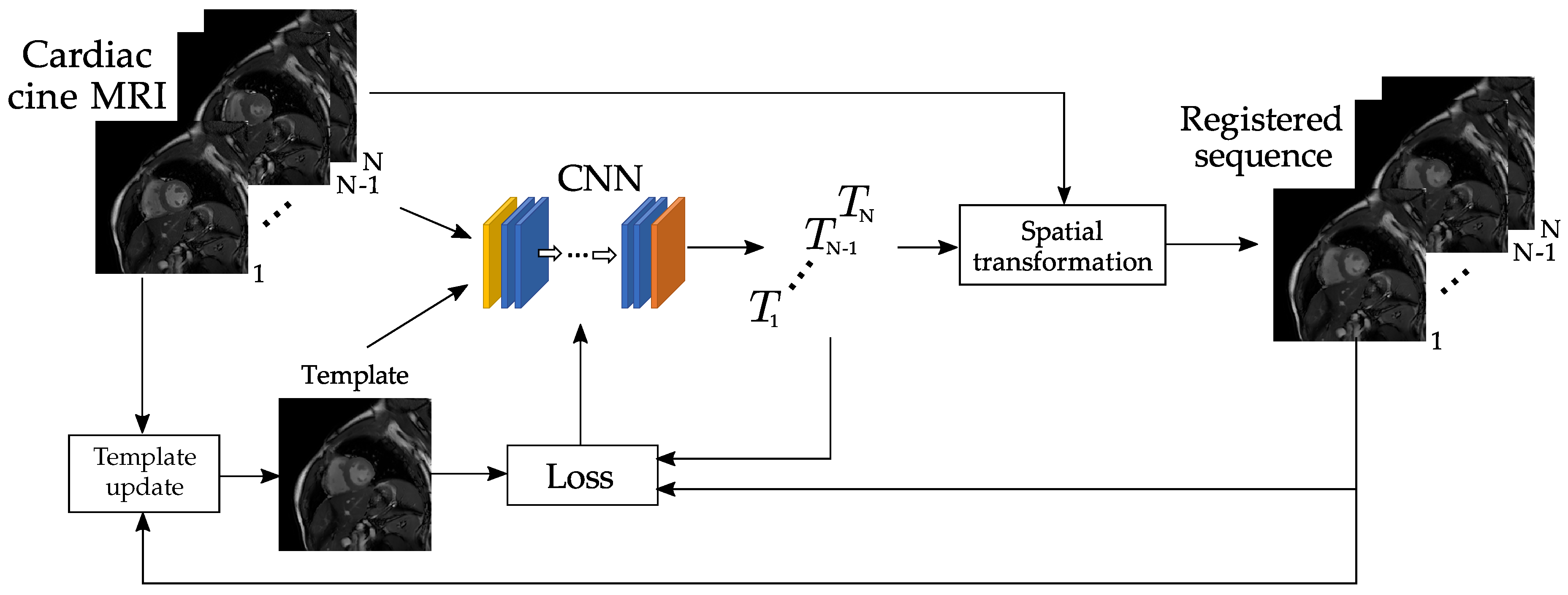
Abstract
:1. Introduction
2. Related Work
3. Material and Methods
3.1. Materials
3.2. Reconstruction Problem
3.3. Registration
3.4. Registration via Deep Learning
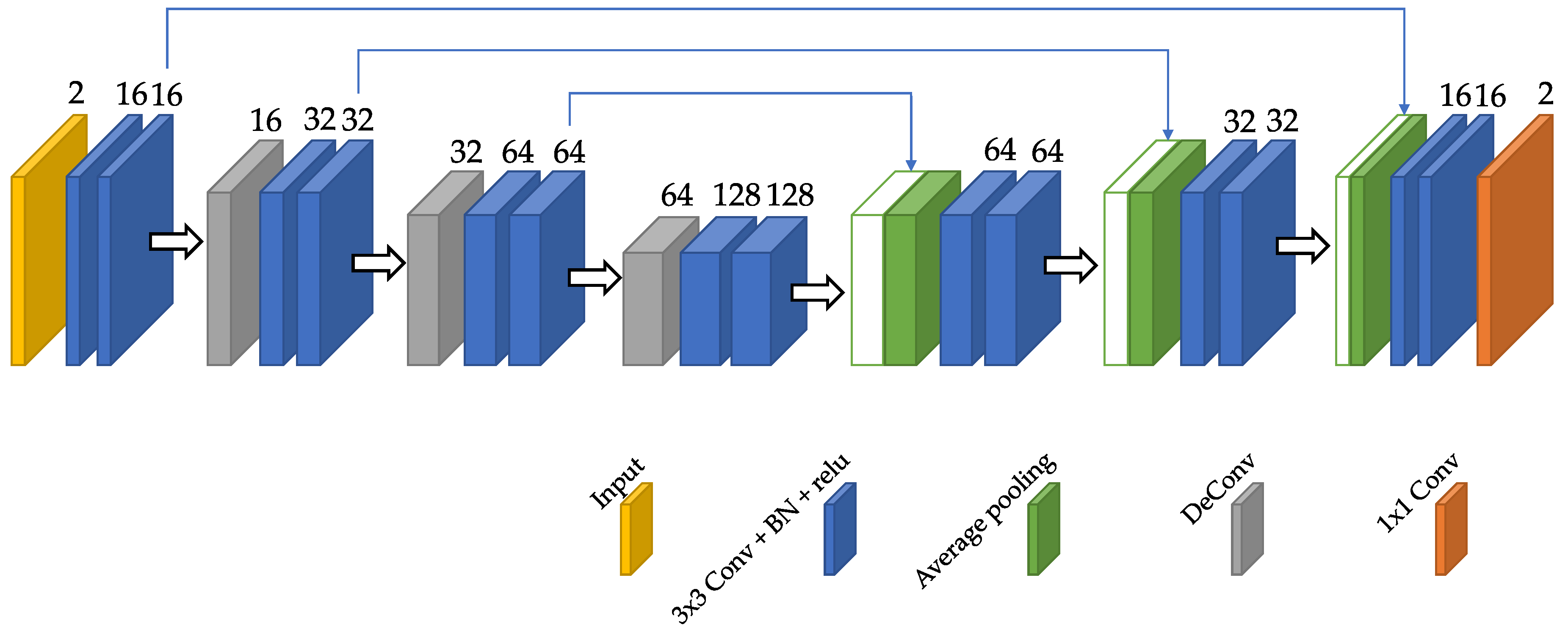
3.4.1. Architecture
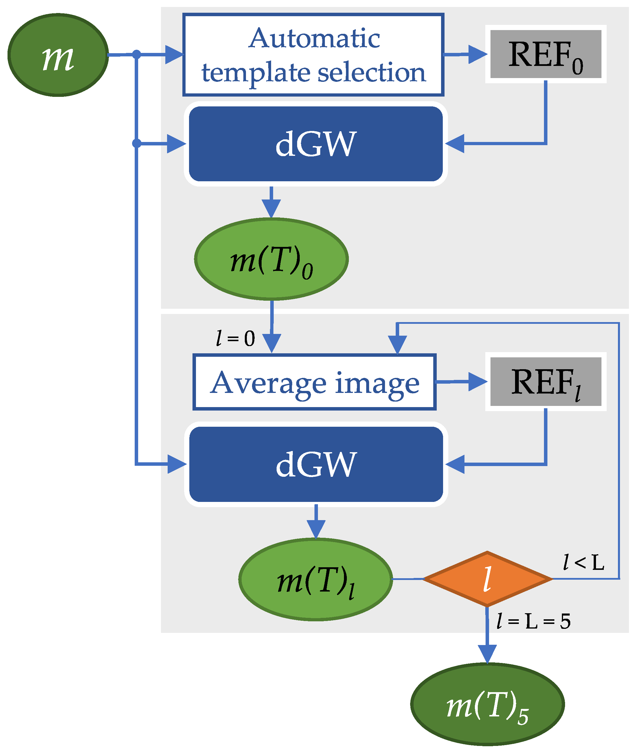
3.4.2. Template Update
- (a)
- Define the similarity between two frames as the residual complexity [27].
- (b)
- Construct the connected kNN graph of frames based on that similarity, where k is the number of neighbors of each frame. A frame is considered connected to its k-closest frames, the higher k, the more connected the graph.
- (c)
- Compute the geodesic distance of every node in the graph.
- (d)
- Select the node, i.e., the frame, with a minimum sum of distances to the rest of the frames. This frame will be taken as the template.
3.4.3. Loss Function
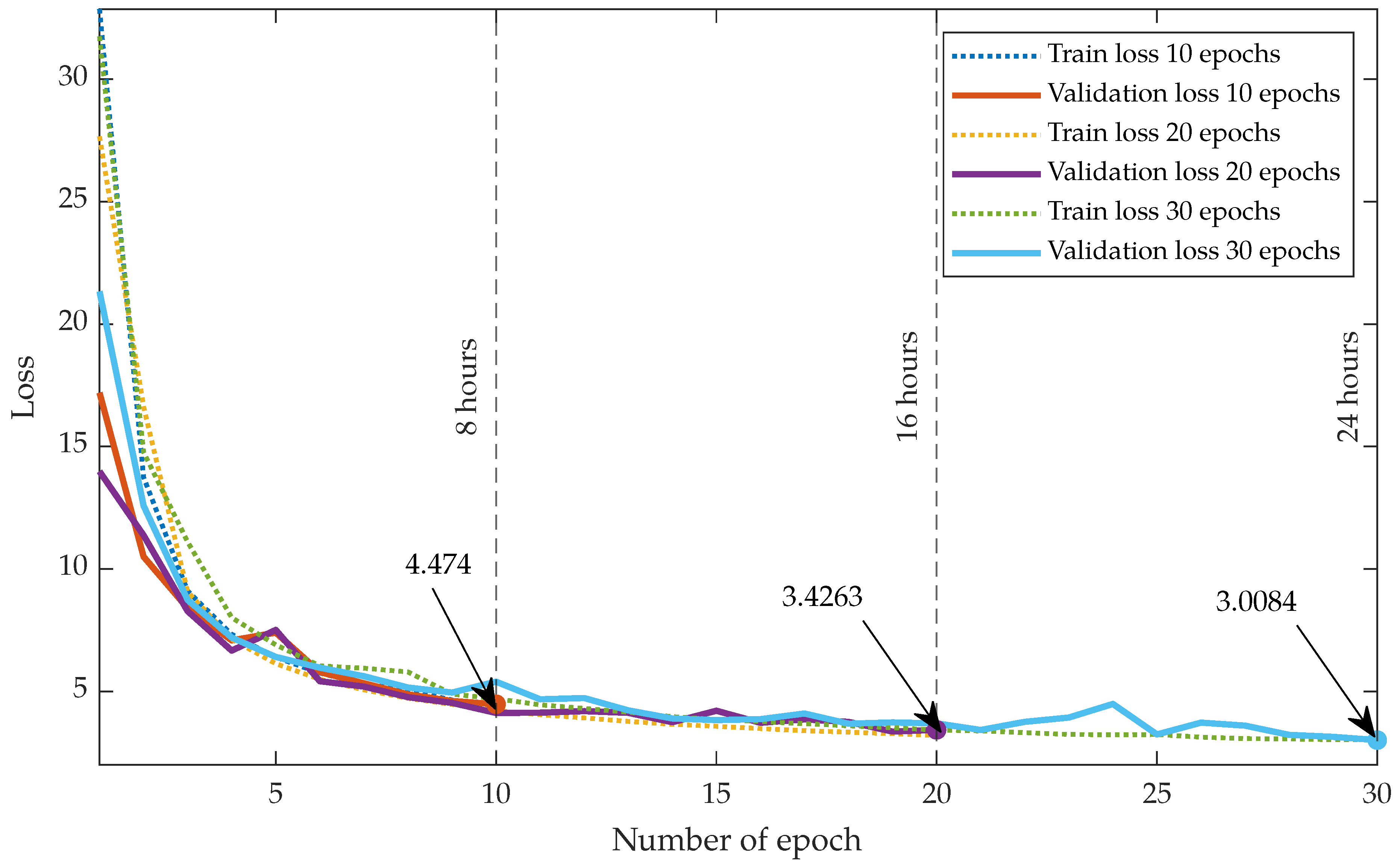
3.4.4. Training
- Set . The template is calculated as described in Section 3.4.2.
- The batch size is taken as the number of frames per slice; therefore, following the definition of iteration given in Section 3.4, network parameters are updated at the end of each iteration; at this moment, the registered sequence is obtained.
- Set . Update the template as the average of the registered sequence at the previous iteration.
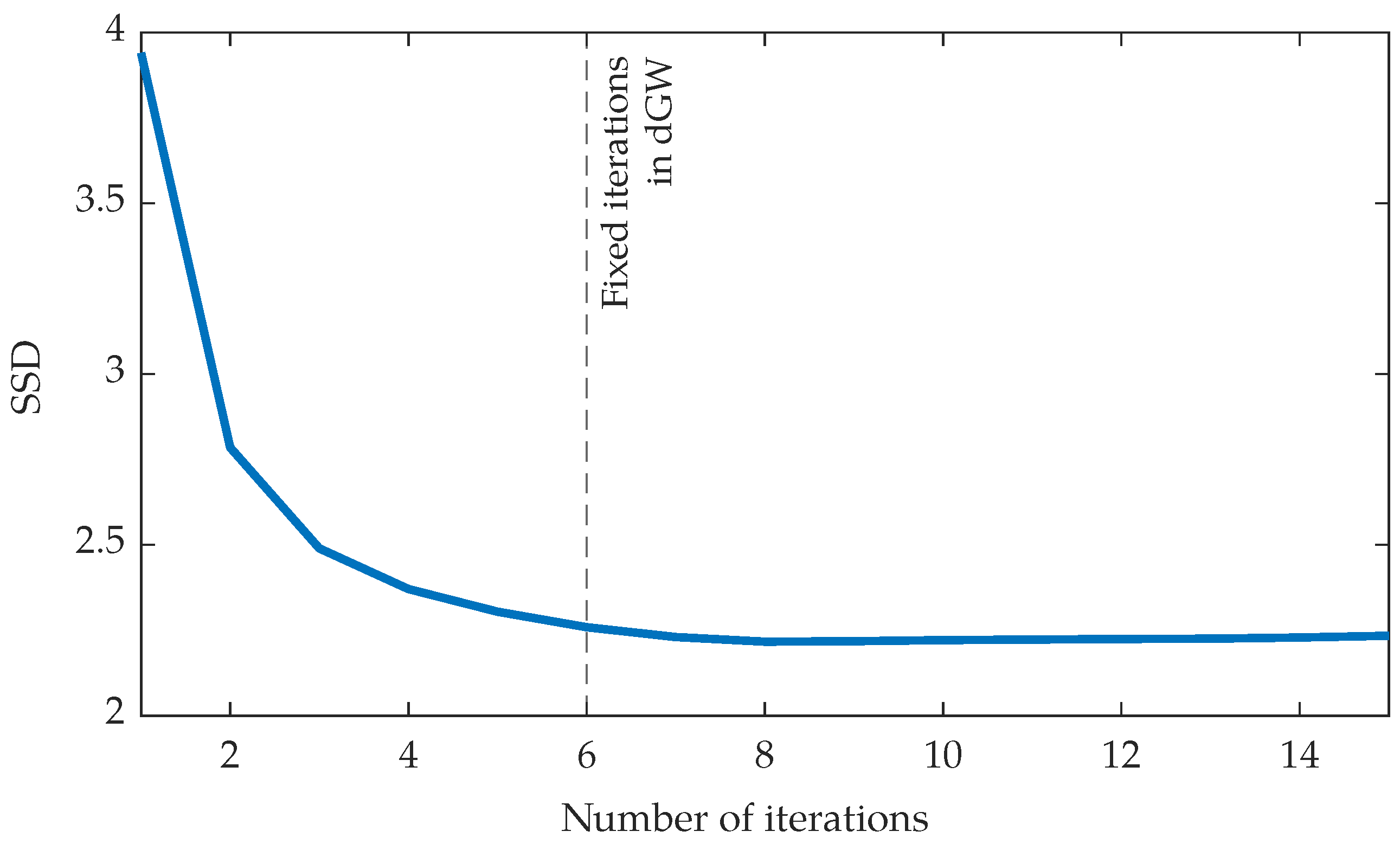
- Steps 2 and 3 are executed while ; consequently, 6 templates are calculated for a given slice. The output at this stage is considered to be the final registration output. The number is a parameter design that has been set beforehand.
3.4.5. Implementation
3.5. Performance Analysis and Hyperparameter Selection
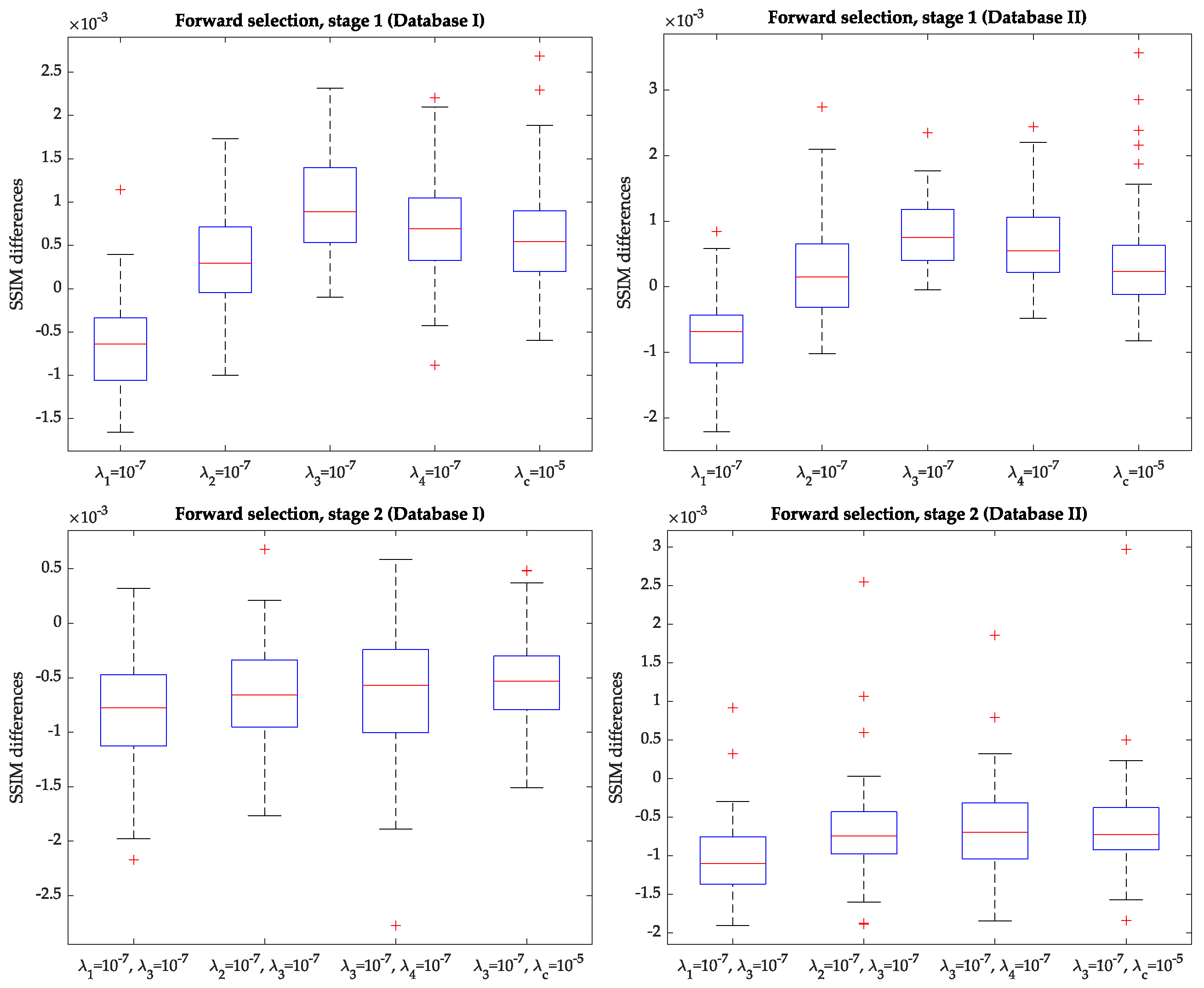
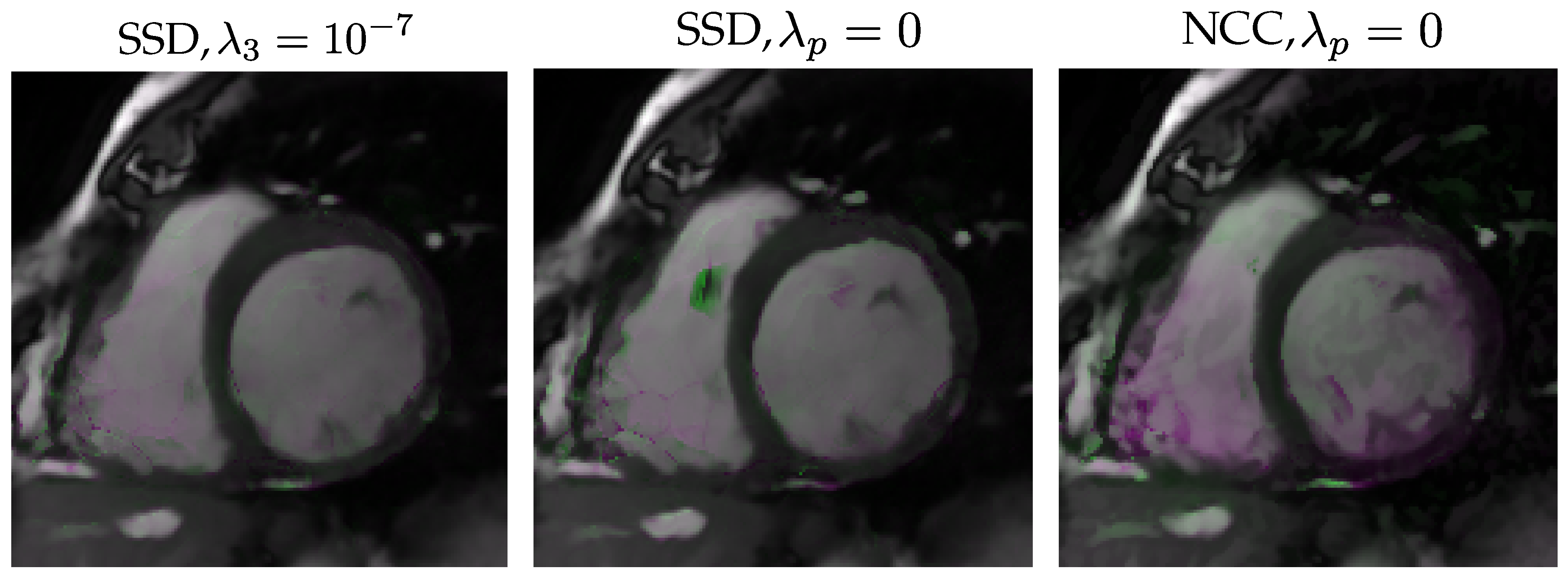
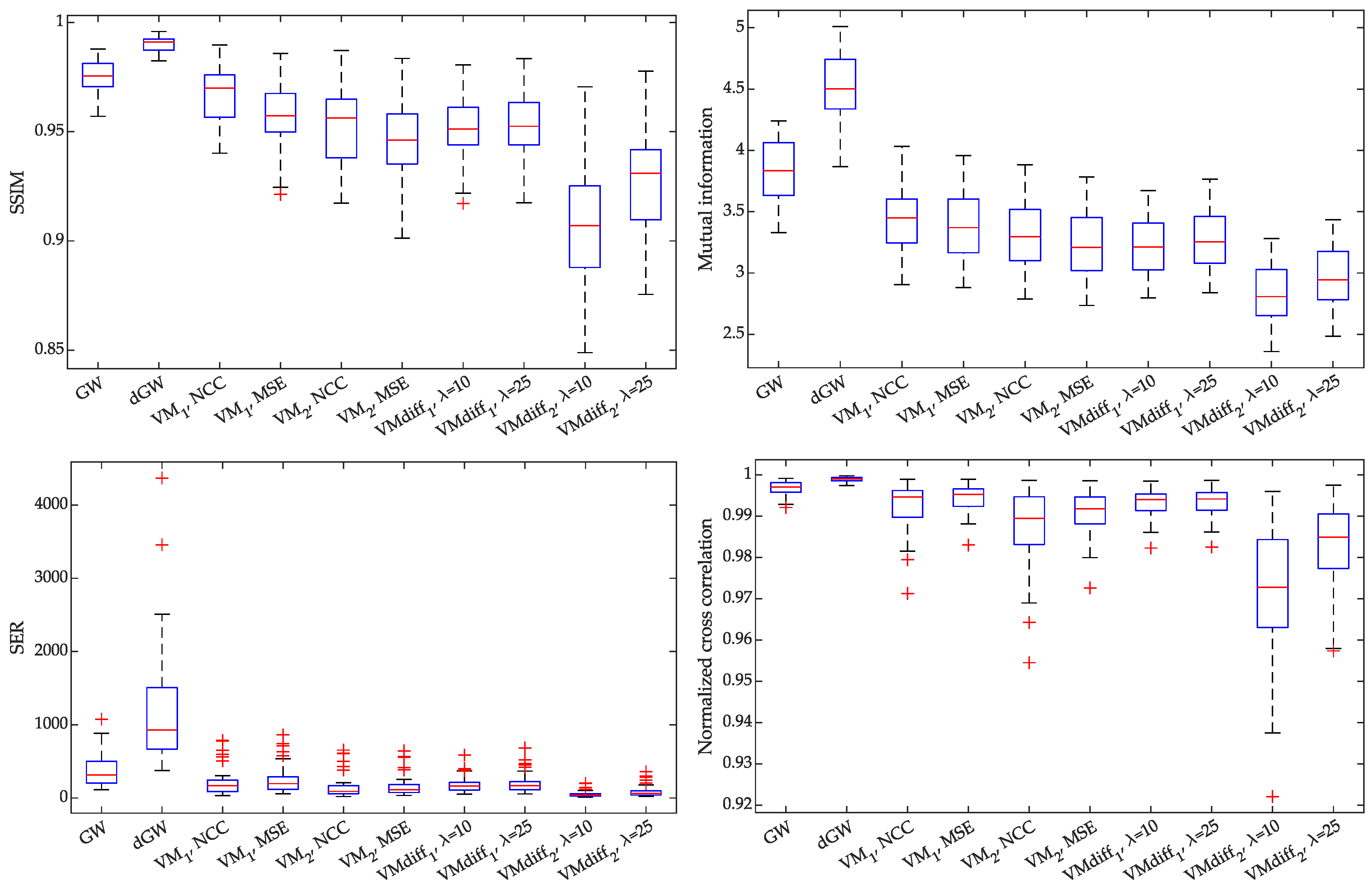
- Stage one: we pursue to find the optimum value of each hyperparameter while the others are null. Then, the best among them is selected. For the four parameters in Equation (6), we test the values ; for in Equation (10) we tried ; these values were preselected on the basis of the validation set in Database I. Then, for each hyperparameter and each value within the pairs just mentioned, we train a network and then a SSIM sample is obtained with each validation dataset. Notice that networks are trained. SSIM values turned out to be quite close to the all-null solution indicated in Stage 0. Thus, we have obtained the boxplots of the pairwise differences between the SSIM sample with each parameter taking a non-null value and the SSIM sample obtained from the network in Stage 0. Figure 5, upper row, shows these boxplots for the validation sets in Database I (left) and Database II (right) for the best selection of each parameter within the pair indicated above (i.e., for the value of this parameter that provides the most favorable result to this parameter); clearly, turns out not to be relevant, while the others provide positive-shifted distributions; in the four rightmost boxplots differences turned out to be significant with p-values . As can be appraised, the highest median corresponds to the activation of ; this is observed with the two databases. Hence, the result of this stage is the setting of the first order () temporal derivative defined in Equation (7) to the value .
- Stage two: the purpose is to find whether the combination of two non-null hyperparameters (being one of them ) provides significantly different results than those provided by the network with and the rest of them null. To this end, new networks are trained with fixed while the others can take values within the pairs indicated above. Then, networks are trained and, for each one, a SSIM sample is obtained with each validation dataset. Should significant differences be found, the second hyperparameter would be that value associated with the minimum p-value. Figure 5, lower row, shows the corresponding pairwise differences in this stage for the best selection of each parameter within the pair indicated above for the validation sets in Database I (left) and Database II (right); the figure clearly shows that adding a second parameter does not provide better results than keeping activated on its own since differences are negative. Therefore, the forward selection procedure ends at this stage, with the selection of a network with only one hyperparameter activated.
- Further stages: in the case that two parameters had been selected, this process would continue by setting a third parameter, with the selected two parameters from stage two remaining fixed, and would continue until all the parameters were set or no significant differences were obtained. Since such differences were not found on stage two, no further stages were tested.
4. Experiments
4.1. Experiment 1: Iterations, Time Sequence Ordering and an Alternative Similarity Metric
4.2. Experiment 2: Performance Comparison with Another DL Architecture
4.3. Experiment 3: dGW vs. an Optimization-Based Registration Approach
4.4. Experiment 4: Dynamic Image Reconstruction
5. Results
5.1. Results of Experiment 1
5.2. Results of Experiment 2
5.3. Results of Experiment 3
5.4. Results of Experiment 4
6. Discussion
7. Conclusions and Future Work
Author Contributions
Funding
Conflicts of Interest
References
- Polfliet, M.; Klein, S.; Huizinga, W.; Paulides, M.M.; Niessen, W.J.; Vandemeulebroucke, J. Intrasubject multimodal groupwise registration with the conditional template entropy. Med. Image Anal. 2018, 46, 15–25. [Google Scholar] [CrossRef]
- Alam, F.; Rahman, S.U. Medical image registration: Classification, applications and issues. JPMI 2018, 32, 300. [Google Scholar]
- Metz, C.T.; Klein, S.; Schaap, M.; Van Walsum, T.; Niessen, W.J. Nonrigid registration of dynamic medical imaging data using nD+ t B-splines and a groupwise optimization approach. Med. Image Anal. 2011, 15, 238–249. [Google Scholar] [CrossRef]
- Che, T.; Zheng, Y.; Cong, J.; Jiang, Y.; Niu, Y.; Jiao, W.; Zhao, B.; Ding, Y. Deep group-wise registration for multi-spectral images from fundus images. IEEE Access 2019, 7, 27650–27661. [Google Scholar] [CrossRef]
- Balakrishnan, G.; Zhao, A.; Sabuncu, M.R.; Guttag, J.; Dalca, A.V. VoxelMorph: A learning framework for deformable medical image registration. IEEE Trans. Med. Imaging 2019, 38, 1788–1800. [Google Scholar] [CrossRef] [Green Version]
- Dalca, A.V.; Balakrishnan, G.; Guttag, J.; Sabuncu, M.R. Unsupervised learning of probabilistic diffeomorphic registration for images and surfaces. Med. Image Anal. 2019, 57, 226–236. [Google Scholar] [CrossRef] [Green Version]
- Royuela-del Val, J.; Cordero-Grande, L.; Simmross-Wattenberg, F.; Martín-Fernández, M.; Alberola-López, C. Nonrigid groupwise registration for motion estimation and compensation in compressed sensing reconstruction of breath-hold cardiac cine MRI. Magn. Reson. Med. 2016, 75, 1525–1536. [Google Scholar] [CrossRef] [Green Version]
- Guyader, J.M.; Huizinga, W.; Poot, D.H.; Van Kranenburg, M.; Uitterdijk, A.; Niessen, W.J.; Klein, S. Groupwise image registration based on a total correlation dissimilarity measure for quantitative MRI and dynamic imaging data. Sci. Rep. 2018, 8, 13112. [Google Scholar] [CrossRef]
- Pontré, B.; Cowan, B.R.; DiBella, E.; Kulaseharan, S.; Likhite, D.; Noorman, N.; Tautz, L.; Tustison, N.; Wollny, G.; Young, A.A.; et al. An open benchmark challenge for motion correction of myocardial perfusion MRI. IEEE J. Biomed. Health Inform. 2016, 21, 1315–1326. [Google Scholar] [CrossRef]
- Hu, Y.; Modat, M.; Gibson, E.; Li, W.; Ghavami, N.; Bonmati, E.; Wang, G.; Bandula, S.; Moore, C.M.; Emberton, M.; et al. Weakly-supervised convolutional neural networks for multimodal image registration. Med. Image Anal. 2018, 49, 1–13. [Google Scholar] [CrossRef]
- Zhao, S.; Lau, T.; Luo, J.; Eric, I.; Chang, C.; Xu, Y. Unsupervised 3d end-to-end medical image registration with volume tweening network. IEEE J. Biomed. Health Inform. 2019, 24, 1394–1404. [Google Scholar] [CrossRef] [Green Version]
- Krebs, J.; Mansi, T.; Mailhé, B.; Ayache, N.; Delingette, H. Unsupervised Probabilistic Deformation Modeling for Robust Diffeomorphic Registration. In Deep Learning in Medical Image Analysis and Multimodal Learning for Clinical Decision Support; Springer: Cham, Switzerland, 2018. [Google Scholar]
- Ahmad, S.; Fan, J.; Dong, P.; Cao, X.; Yap, P.T.; Shen, D. Deep Learning Deformation Initialization for Rapid Groupwise Registration of Inhomogeneous Image Populations. Front. Neuroinform. 2019, 13, 34. [Google Scholar]
- Siebert, H.; Heinrich, M.P. Deep Groupwise Registration of MRI Using Deforming Autoencoders. In Bildverarbeitung für die Medizin 2020; Tolxdorff, T., Deserno, T.M., Handels, H., Maier, A., Maier-Hein, K.H., Palm, C., Eds.; Springer: Wiesbaden, Germany, 2020; pp. 236–241. [Google Scholar]
- Feng, L.; Coppo, S.; Piccini, D.; Yerly, J.; Lim, R.P.; Masci, P.G.; Stuber, M.; Sodickson, D.K.; Otazo, R. 5D whole-heart sparse MRI. Magn. Reson. Med. 2018, 79, 826–838. [Google Scholar] [CrossRef] [PubMed]
- Asif, M.S.; Hamilton, L.; Brummer, M.; Romberg, J. Motion-adaptive spatio-temporal regularization for accelerated dynamic MRI. Magn. Reson. Med. 2013, 70, 800–812. [Google Scholar] [CrossRef]
- Menchón-Lara, R.M.; Royuela del Val, J.; Godino-Moya, A.; Cordero-Grande, L.; Simmross-Wattenberg, F.; Martin-Fernandez, M.; Alberola-López, C. An Efficient Multi-resolution Reconstruction Scheme with Motion Compensation for 5D Free-Breathing Whole-Heart MRI. In Molecular Imaging, Reconstruction and Analysis of Moving Body Organs, and Stroke Imaging and Treatment; Springer: Cham, Switzerland, 2017; pp. 136–145. [Google Scholar] [CrossRef]
- Schlemper, J.; Caballero, J.; Hajnal, J.V.; Price, A.N.; Rueckert, D. A deep cascade of convolutional neural networks for dynamic MR image reconstruction. IEEE Trans. Med. Imaging 2017, 37, 491–503. [Google Scholar] [CrossRef] [PubMed] [Green Version]
- Qin, C.; Schlemper, J.; Caballero, J.; Price, A.N.; Hajnal, J.V.; Rueckert, D. Convolutional recurrent neural networks for dynamic MR image reconstruction. IEEE Trans. Med. Imaging 2018, 38, 280–290. [Google Scholar] [CrossRef] [PubMed] [Green Version]
- Aggarwal, H.K.; Mani, M.P.; Jacob, M. MoDL: Model-based deep learning architecture for inverse problems. IEEE Trans. Med. Imaging 2018, 38, 394–405. [Google Scholar] [CrossRef]
- Martín-González, E.; Casaseca-de-la Higuera, P.; San-José-Revuelta, L.M.; Alberola-López, C. Groupwise Deep Learning-based Approach for Motion Compensation. Application to Compressed Sensing 2D Cardiac Cine MRI Reconstruction. In Proceedings of the XXXVII Congreso Anual de la Sociedad Española de Ingeniería Biomédica, Santander, Spain, 27–29 November 2019; pp. 299–302. [Google Scholar]
- Sanz-Estébanez, S.; Cordero-Grande, L.; Sevilla, T.; Revilla-Orodea, A.; De Luis-García, R.; Martín-Fernández, M.; Alberola-López, C. Vortical features for myocardial rotation assessment in hypertrophic cardiomyopathy using cardiac tagged magnetic resonance. Med. Image Anal. 2018, 47, 191–202. [Google Scholar] [CrossRef] [Green Version]
- Royuela-del Val, J.; Cordero-Grande, L.; Simmross-Wattenberg, F.; Martín-Fernández, M.; Alberola-López, C. Jacobian weighted temporal total variation for motion compensated compressed sensing reconstruction of dynamic MRI. Magn. Reson. Med. 2017, 77, 1208–1215. [Google Scholar] [CrossRef] [Green Version]
- Rueckert, D.; Sonoda, L.I.; Hayes, C.; Hill, D.L.; Leach, M.O.; Hawkes, D.J. Nonrigid registration using free-form deformations: Application to breast MR images. IEEE Trans. Med. Imaging 1999, 18, 712–721. [Google Scholar] [CrossRef]
- Cordero-Grande, L.; Merino-Caviedes, S.; Aja-Fernández, S.; Alberola-López, C. Groupwise elastic registration by a new sparsity-promoting metric: Application to the alignment of cardiac magnetic resonance perfusion images. IEEE Trans. Pattern Anal. Mach. Intell. 2013, 35, 2638–2650. [Google Scholar] [CrossRef]
- Ronneberger, O.; Fischer, P.; Brox, T. U-Net: Convolutional Networks for Biomedical Image Segmentation. In Proceedings of the International Conference on Medical Image Computing and Computer-Assisted Intervention, Munich, Germany, 5–9 October 2015; Springer: Cham, Switzerland, 2015. [Google Scholar]
- Feng, Q.; Zhou, Y.; Li, X.; Mei, Y.; Lu, Z.; Zhang, Y.; Feng, Y.; Liu, Y.; Yang, W.; Chen, W. Liver DCE-MRI registration in manifold space based on robust principal component analysis. Sci. Rep. 2016, 6, 34461. [Google Scholar] [CrossRef] [PubMed] [Green Version]
- Bhatia, K.K.; Hajnal, J.V.; Puri, B.K.; Edwards, A.D.; Rueckert, D. Consistent groupwise non-rigid registration for atlas construction. In Proceedings of the 2004 2nd IEEE International Symposium on Biomedical Imaging: Nano to Macro (IEEE Cat No. 04EX821), Arlington, VA, USA, 18 April 2004; pp. 908–911. [Google Scholar]
- Abadi, M.; Agarwal, A.; Barham, P.; Brevdo, E.; Chen, Z.; Citro, C.; Corrado, G.S.; Davis, A.; Dean, J.; Devin, M.; et al. TensorFlow: Large-Scale Machine Learning on Heterogeneous Systems. 2015. Available online: tensorflow.org (accessed on 17 June 2020).
- Keras. 2015. Available online: https://keras.io (accessed on 17 June 2020).
- Kingma, D.P.; Ba, J. Adam: A Method for Stochastic Optimization. arXiv 2014, arXiv:1412.6980. [Google Scholar]
- Dalca, A.V.; Guttag, J.; Sabuncu, M.R. Anatomical priors in convolutional networks for unsupervised biomedical segmentation. In Proceedings of the IEEE Conference on Computer Vision and Pattern Recognition, Salt Lake City, UT, USA, 18–22 June 2018; pp. 9290–9299. [Google Scholar]
- Wang, Z.; Bovik, A.C.; Sheikh, H.R.; Simoncelli, E.P. Image quality assessment: From error visibility to structural similarity. IEEE Trans. Image Process. 2004, 13, 600–612. [Google Scholar] [CrossRef] [PubMed] [Green Version]
- Theodoridis, S.; Koutroumbas, K. Pattern Recognition, Copyright 2003; Elsevier: Amsterdam, The Netherlands, 2003. [Google Scholar]
- Cover, T.M.; Thomas, J.A. Entropy, relative entropy and mutual information. Elem. Inf. Theory 1991, 2, 1–55. [Google Scholar]
- Lewis, J. Industrial Light & Magic. Fast Norm. Cross Correl. 1995, 2011, 1. [Google Scholar]
- Yang, X.; Kwitt, R.; Styner, M.; Niethammer, M. Quicksilver: Fast predictive image registration—A deep learning approach. NeuroImage 2017, 158, 378–396. [Google Scholar] [CrossRef]
- Sokooti, H.; De Vos, B.; Berendsen, F.; Lelieveldt, B.P.; Išgum, I.; Staring, M. Nonrigid image registration using multi-scale 3D convolutional neural networks. In Proceedings of the International Conference on Medical Image Computing and Computer-Assisted Intervention, Quebec City, QC, Canada, 10–14 September 2017; Springer: Cham, Switzerland, 2017; pp. 232–239. [Google Scholar]
- Wu, G.; Kim, M.; Wang, Q.; Munsell, B.C.; Shen, D. Scalable high-performance image registration framework by unsupervised deep feature representations learning. IEEE Trans. Biomed. Eng. 2015, 63, 1505–1516. [Google Scholar] [CrossRef] [Green Version]


© 2020 by the authors. Licensee MDPI, Basel, Switzerland. This article is an open access article distributed under the terms and conditions of the Creative Commons Attribution (CC BY) license (http://creativecommons.org/licenses/by/4.0/).
Share and Cite
Martín-González, E.; Sevilla, T.; Revilla-Orodea, A.; Casaseca-de-la-Higuera, P.; Alberola-López, C. Groupwise Non-Rigid Registration with Deep Learning: An Affordable Solution Applied to 2D Cardiac Cine MRI Reconstruction. Entropy 2020, 22, 687. https://0-doi-org.brum.beds.ac.uk/10.3390/e22060687
Martín-González E, Sevilla T, Revilla-Orodea A, Casaseca-de-la-Higuera P, Alberola-López C. Groupwise Non-Rigid Registration with Deep Learning: An Affordable Solution Applied to 2D Cardiac Cine MRI Reconstruction. Entropy. 2020; 22(6):687. https://0-doi-org.brum.beds.ac.uk/10.3390/e22060687
Chicago/Turabian StyleMartín-González, Elena, Teresa Sevilla, Ana Revilla-Orodea, Pablo Casaseca-de-la-Higuera, and Carlos Alberola-López. 2020. "Groupwise Non-Rigid Registration with Deep Learning: An Affordable Solution Applied to 2D Cardiac Cine MRI Reconstruction" Entropy 22, no. 6: 687. https://0-doi-org.brum.beds.ac.uk/10.3390/e22060687