A New Look on Financial Markets Co-Movement through Cooperative Dynamics in Many-Body Physics

 ,
,  ,
,  , and
, and 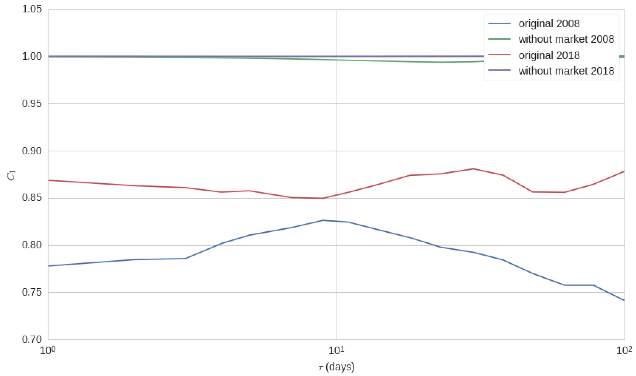
Abstract
:1. Introduction
- is the return on the asset i,
- is the part of the return on the asset i that is due to aspects of the asset itself, such as profit, business, etc.
- is the return of the risk-free asset,
- is the market return (usually proxied through its main equity index or an all-shares value-weighted portfolio),
- is known as the market risk premium, and
- is a zero-mean residual.
2. Methodology
- . Consider the functionswhere is the log-price of asset i at time t, and the sum is for each pair of assets i, j, excluding the pairs i, i. is the average of over time origins t.The function is a measure of co-movement, from time t to time , along the time t and the function is a measure of co-movement for the full period considered.The interpretation of these functions is as follows: if the resulting function is close to 1, it means that there is no co-movement in the whole market; if it yields values lower than 1, then we can say that the stocks move together; and if, on the contrary, the values are greater than 1, the stocks tend to move in the opposite direction.
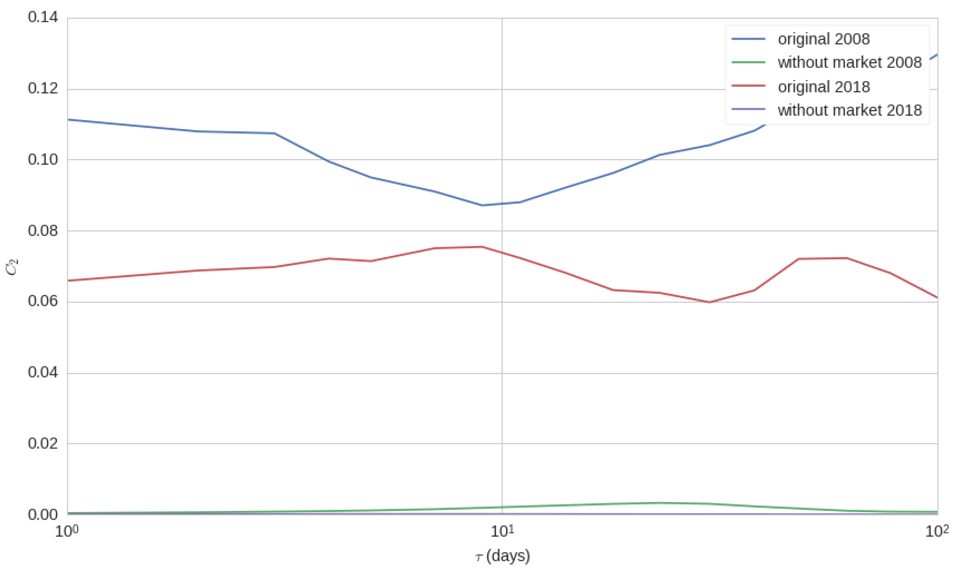
- . Consider the functionswhere the same notation is used.In this case, if the functions are close to 0 it means that there is no co-movement; if they are greater than 0, it means that the stocks move in the same direction and, when they are less than 0, the stocks move in the opposite direction.
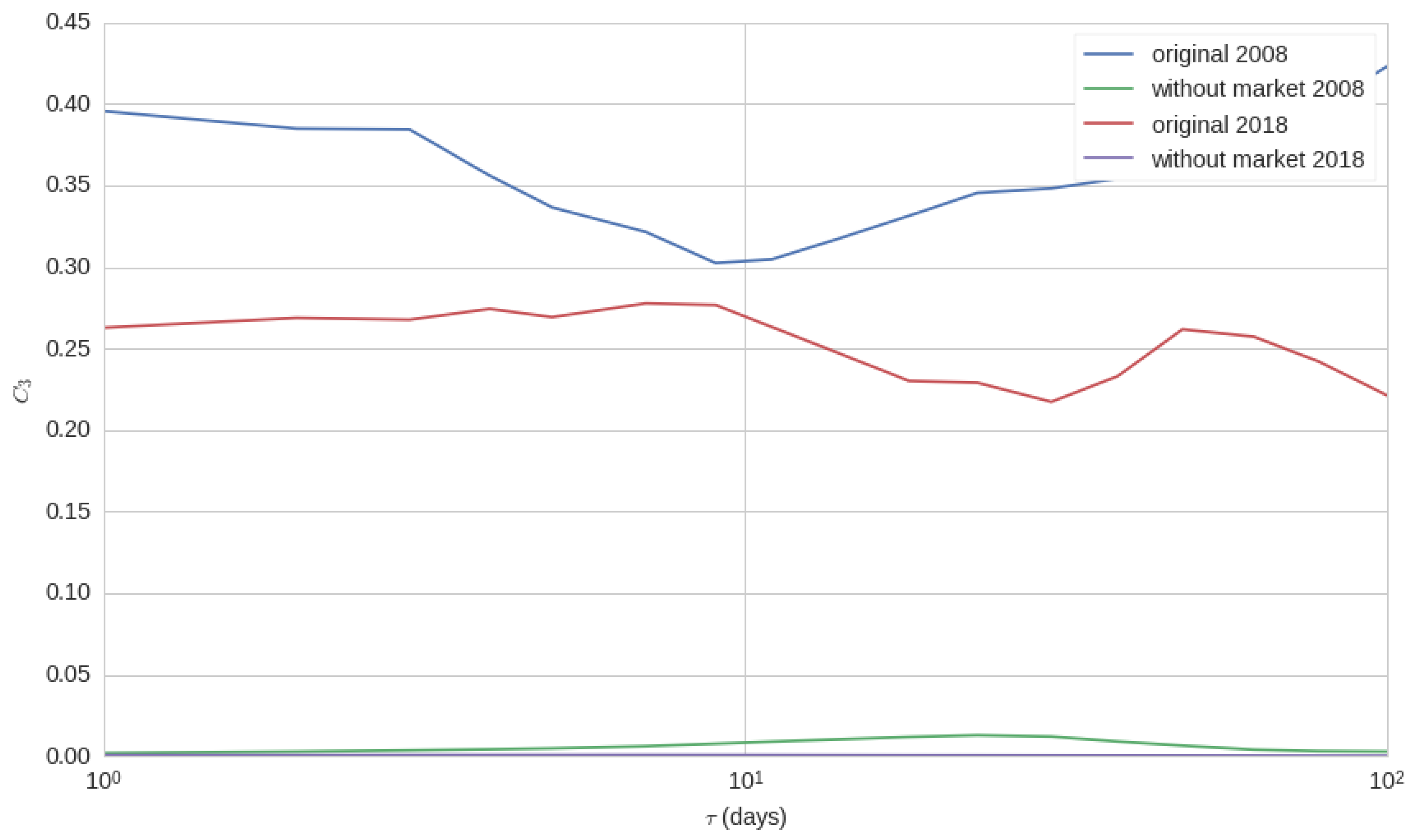
- . Consider the functionswhere the same notation is used.These functions are interpreted in the same way that . Note that and take values between and 1.
3. Results
3.1. Co-Movement for Different Lag Times with and without Considering the Market
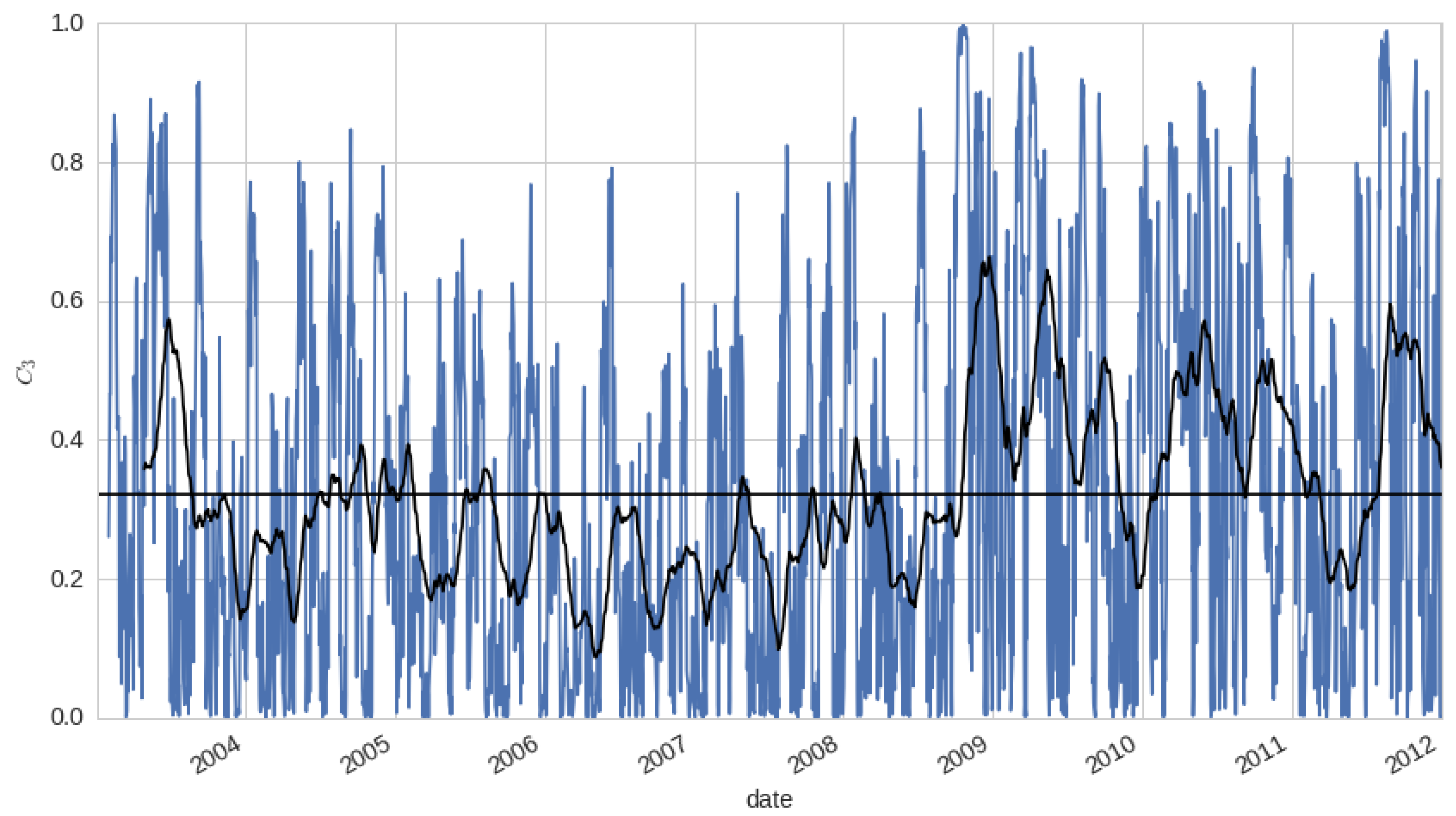
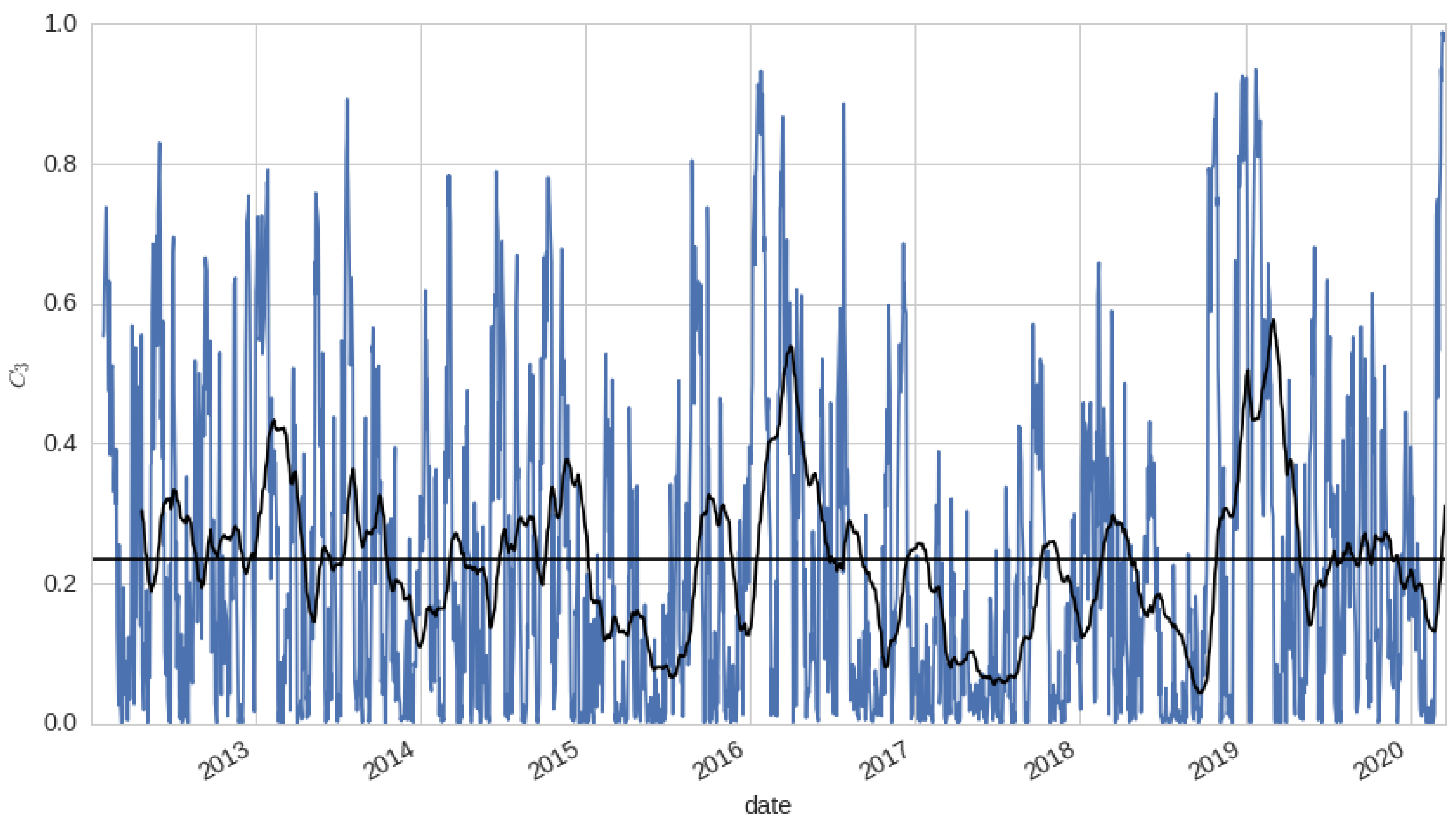
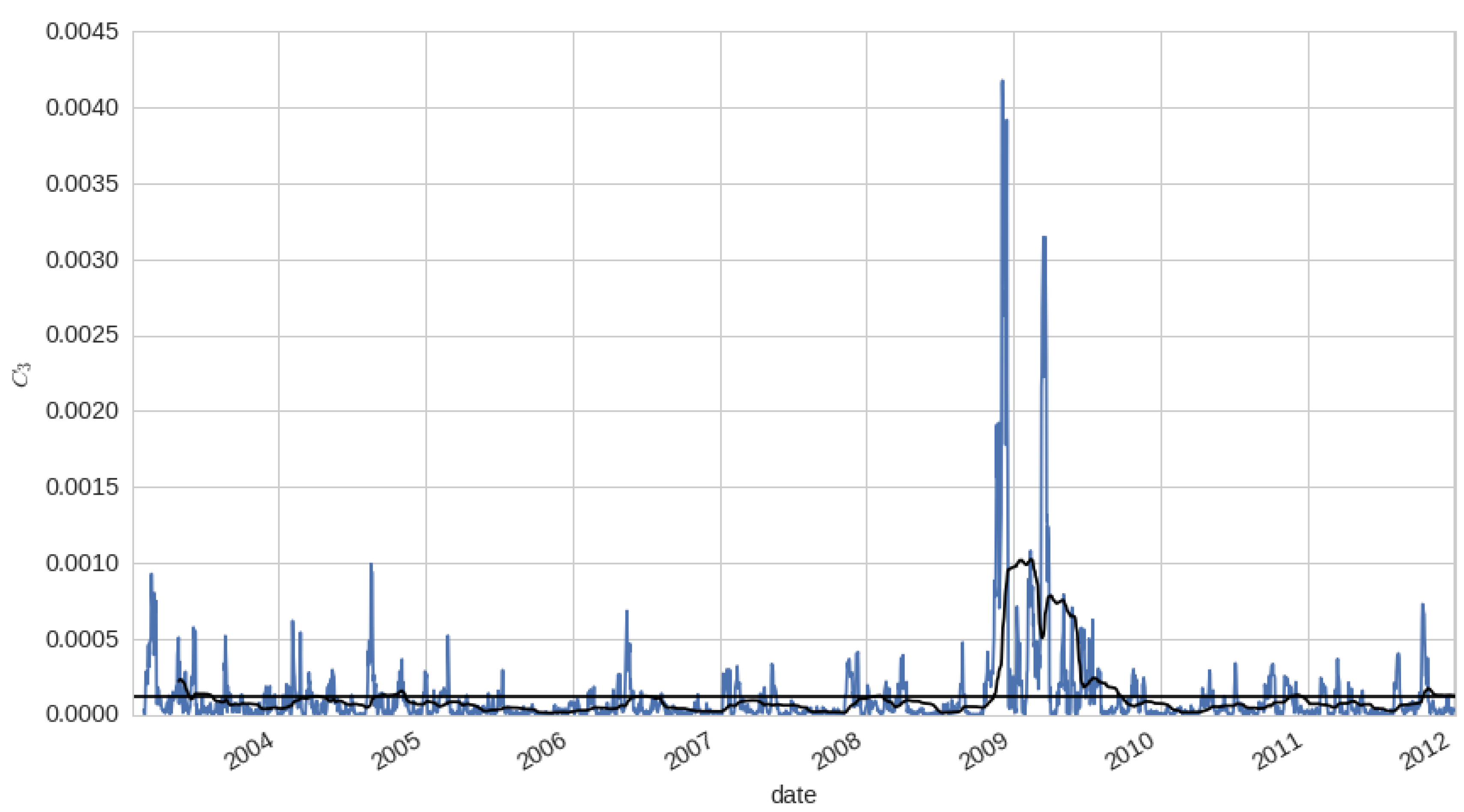
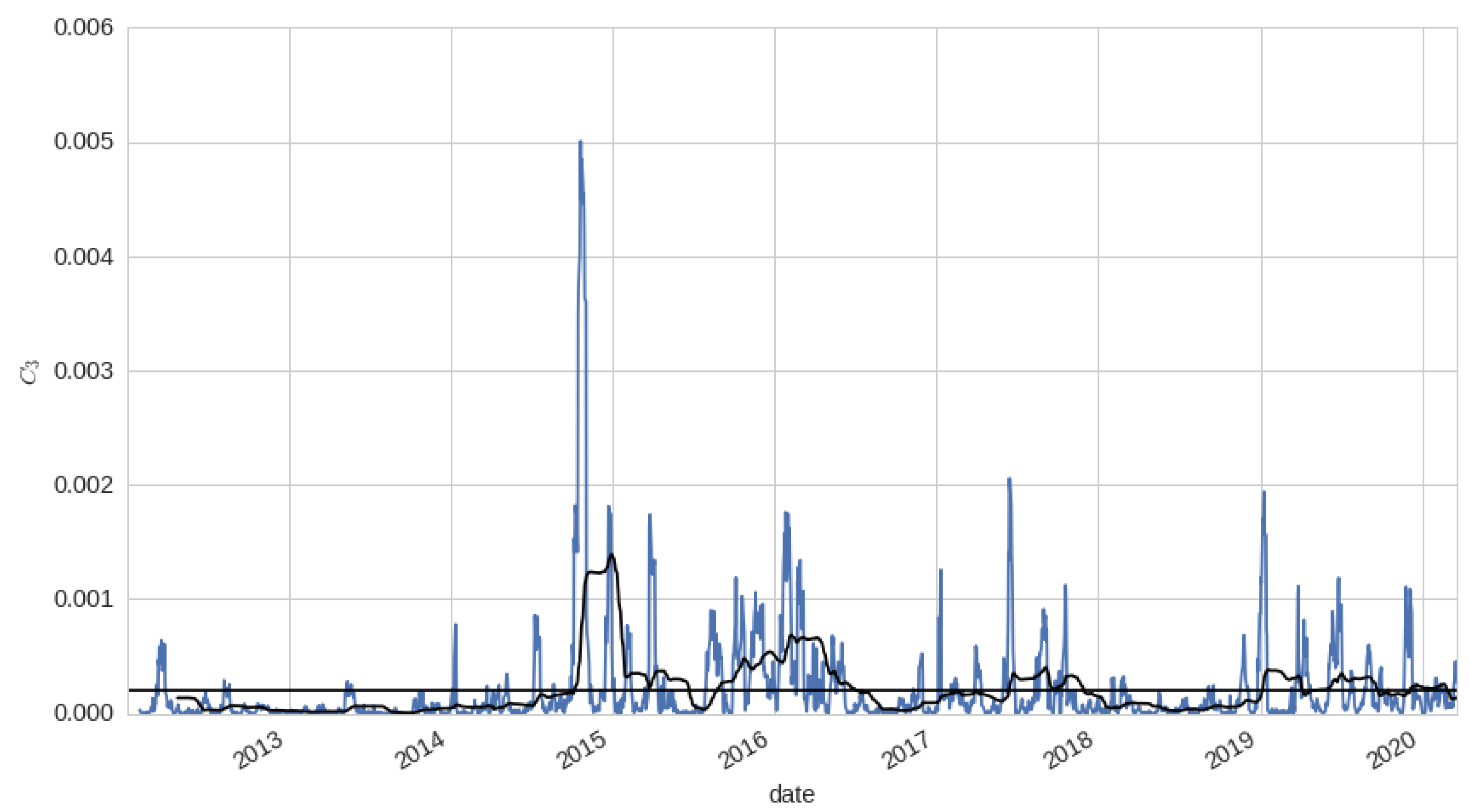
3.2. Co-Movement along the Time
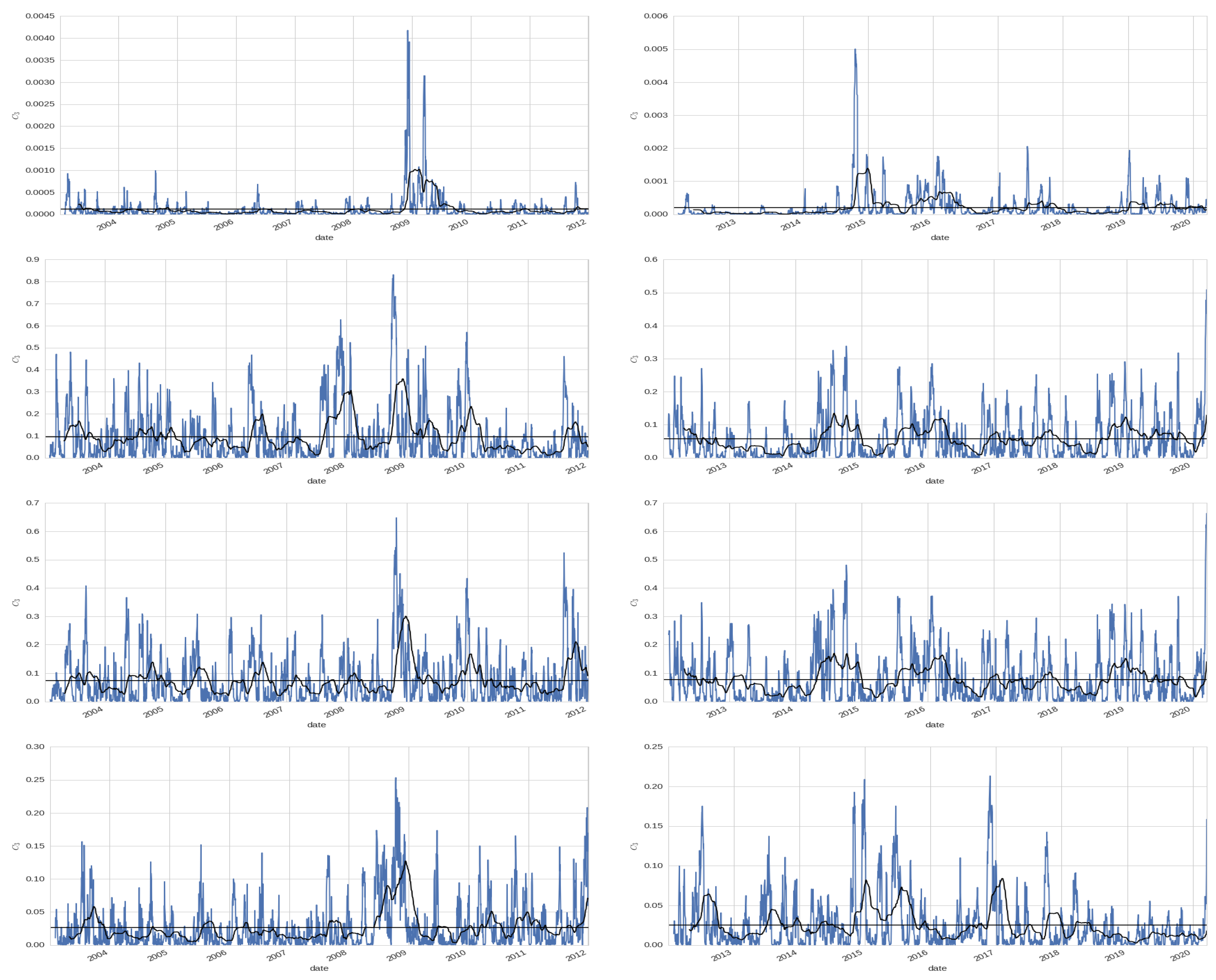
3.3. Other Ways to Represent the Market
- ew: equal weight. This is the representation described in the previous section, which is, , where is the number of stocks at time t.
- cap: this representation is calculated as a capitalization-weighted average, which is, and with the capitalization of asset j.
- SPY: the SP500 index.
- IWM: the Russell 2000 index.
Considering Beta
4. Conclusions
Author Contributions
Funding
Conflicts of Interest
References
- Sharpe, W. Capital Asset Prices: A theory of market equilibrium under conditions of risk. J. Financ. 1964, 19, 425–442. [Google Scholar]
- Lintner, J. The valuation of risk assets and the selection of risky investments in stock portfolios and capital budgets. Rev. Econ. Stat. 1965, 47, 13–37. [Google Scholar] [CrossRef]
- Black, F. Capital Market Equilibrium with Restricted Borrowing. J. Bus. 1972, 45, 444–455. [Google Scholar] [CrossRef] [Green Version]
- Black, F. Beta and returns. J. Portf. Manag. Fall 1993, 20, 8–18. [Google Scholar] [CrossRef]
- Blume, M. On the assessment f risk. J. Financ. 1971, 26, 1–10. [Google Scholar] [CrossRef]
- Black, F.; Jensen, M.; Scholes, M. The capital asset pricing model: Some empirical tests. Stud. Theory Cap. Mark. 1972, 81, 79–121. [Google Scholar]
- Fama, E.F.; MacBeth, J.D. Risk, Return, and Equilibrium: Empirical Tests. J. Political Econ. 1973, 81, 607–636. [Google Scholar] [CrossRef]
- King, B.F. Market and Industry Factors in Stock Price Behavior. J. Bus. 1966, 39, 139–190. [Google Scholar] [CrossRef] [Green Version]
- Meyers, S.L. A Re-Examination of Market and Industry Factors in Stock Price Behavior. J. Financ. 1973, 28, 695–705. [Google Scholar] [CrossRef]
- Banz, R.W. The relationship between return and market value of common stocks. J. Financ. Econ. 1981, 9, 3–18. [Google Scholar] [CrossRef] [Green Version]
- Roll, R. R2. J. Financ. 1988, 43, 541–566. [Google Scholar] [CrossRef]
- Bhandari, L.C. Debt/Equity Ratio and Expected Common Stock Returns: Empirical Evidence. J. Financ. 1988, 43, 507–528. [Google Scholar] [CrossRef]
- Stattman, D. Book values and stocks returns. Chic. MBA J. Sel. Pap. 1980, 4, 25–45. [Google Scholar]
- Rosenberg, B.; Reid, K.; Lanstein, R. Persuasive Evidence of Market Inefficiency. J. Portf. Manag. 1985, 11, 9–17. [Google Scholar] [CrossRef]
- Fama, E.F.; French, K.R. The Cross-Section of Expected Stock Returns. J. Financ. 1992, 47, 427–465. [Google Scholar] [CrossRef]
- Isakov, D. Is beta still alive? Conclusive evidence from the Swiss stock market. Eur. J. Financ. 1999, 5, 202–212. [Google Scholar] [CrossRef]
- Pettengill, G.N.; Sundaram, S.; Mathur, I. The Conditional Relation between Beta and Returns. J. Financ. Quant. Anal. 1995, 30, 101–116. [Google Scholar] [CrossRef] [Green Version]
- Chan, L.; Lakonishok, J. Institutional trades and intraday stock price behavior. J. Financ. Econ. 1993, 33, 173–199. [Google Scholar] [CrossRef] [Green Version]
- Grundy, K.; Malkiel, B.G. Reports of beta’s death have been greatly exaggerated. J. Portf. Manag. 1996, 22, 36–44. [Google Scholar] [CrossRef]
- López-García, M.N.; Trinidad-Segovia, J.E.; Sánchez-Granero, M.A.; Pouchkarev, I. Extending the Fama and French model with a long term memory factor. Eur. J. Oper. Res. 2020, in press. [Google Scholar] [CrossRef]
- Domowitz, I.; Hansch, O.; Wang, X. Liquidity commonality and return co-movement. J. Financ. Mark. 2005, 8, 351–376. [Google Scholar] [CrossRef]
- Byrne, J.P.; Cao, S.; Korobilis, D. Decomposing global yield curve co-movement. J. Bank. Financ. 2019, 106, 500–513. [Google Scholar] [CrossRef]
- Morck, R.; Yeung, B.; Yu, W. The information content of stock markets: Why do emerging markets have synchronous stock price movements? J. Financ. Econ. 2000, 58, 215–260. [Google Scholar] [CrossRef] [Green Version]
- Jach, A. International Stock market Comovement Time Scale Outlined A Thick Pen. J. Empir. Financ. 2017, 43, 115–129. [Google Scholar] [CrossRef]
- Parsley, D.; Popper, H. Return comovement. J. Bank. Financ. 2020, 112, 105–223. [Google Scholar] [CrossRef]
- Bonfiglioli, A.; Favero, C.A. Explaining co-movements between stock markets: The case of US and Germany. J. Int. Money Financ. 2005, 24, 1299–1316. [Google Scholar] [CrossRef]
- Rua, A.; Nunes, L.C. International comovement of stock market returns: A wavelet analysis. J. Empir. Financ. 2009, 16, 632–639. [Google Scholar] [CrossRef] [Green Version]
- Akoum, I.; Graham, M.; Kivihaho, J.; Nikkinen, J.; Omran, M. Co-movement of oil and stock prices in the GCC region: A wavelet analysis. Q. Rev. Econ. Financ. 2012, 52, 385–394. [Google Scholar] [CrossRef]
- Reboredo, J.C. Modelling oil prices and exchange rates co-movements. J. Policy Model. 2012, 34, 419–440. [Google Scholar] [CrossRef]
- Magdaleno, M.; Pinho, C. International stock market indices comovements: A new look. Int. J. Financ. Econ. 2012, 17, 89–102. [Google Scholar] [CrossRef]
- Loh, L. Co-movement of Asia-Pacific with European and US stock market returns: A cross-time-frequency analysis. Res. Int. Bus. Financ. 2013, 29, 1–13. [Google Scholar] [CrossRef]
- Baca, S.; Garbe, B.; Weiss, R. The rise of sector effects in major equity markets. Financ. Anal. J. 2000, 56, 35–40. [Google Scholar] [CrossRef]
- Cavaglia, S.; Brightman, C.; Aked, M. The increasing importance of industry factors. Financ. Anal. J. 2000, 56, 41–54. [Google Scholar] [CrossRef] [Green Version]
- Griffin, J.; Karolyi, A. Another look at the role of industrial structure of markets for international diversification strategies. J. Financ. Econ. 1998, 50, 351–373. [Google Scholar] [CrossRef]
- L’Her, J.; Sy, O.; Tnani, Y. Country, industry and risk factor loadings in portfolio management. J. Portf. Manag. 2002, 28, 70–79. [Google Scholar] [CrossRef]
- Brooks, R.; Del Negro, M. Firm-Level Evidence on International Stock Market Comovement. Rev. Financ. 2006, 10, 69–98. [Google Scholar] [CrossRef]
- Antonakakis, N.; Chatziantoniou, I.; Filis, G. Dynamic Co-movements of Stock Market Returns, Implied Volatility and Policy Uncertainty. Econ. Lett. 2013, 120, 87–92. [Google Scholar] [CrossRef]
- Fernández-Avilés Calderón, G.; Montero, J.M.; Orlov, A. Spatial Modeling of Stock Market Comovements. Financ. Res. Lett. 2012, 9, 202–212. [Google Scholar] [CrossRef]
- Cappiello, L.; Gerard, B.; Kadareja, A.; Manganelli, S. Measuring Comovements by Regression Quantiles. J. Financ. Econom. 2014, 12, 645–678. [Google Scholar] [CrossRef]
- Garcia, R.; Tsafack, G. Dependence structure and extreme comovements in international equity and bond markets. J. Bank. Financ. 2011, 35, 1954–1970. [Google Scholar] [CrossRef] [Green Version]
- Fernández-Avilés, G.; Montero, J.M.; Sanchis-Marco, L. Extreme downside risk co-movement in commodity markets during distress periods: A multidimensional scaling approach. Eur. J. Financ. 2020, 12, 1207–1237. [Google Scholar] [CrossRef]
- Ramos Requena, J.P.; Trinidad Segovia, J.E.; Sánchez Granero, M.A. An Alternative Approach to Measure Co-Movement between Two Time Series. Mathematics 2020, 8, 261. [Google Scholar] [CrossRef] [Green Version]
- Clara-Rahola, J.; Puertas, A.M.; Sánchez-Granero, M.A.; Trinidad-Segovia, J.E.; de las Nieves, F.J. Diffusive and arrestedlike dynamics in currency exchange markets. Phys. Rev. Lett. 2017, 118, 068301. [Google Scholar] [CrossRef] [PubMed] [Green Version]
- Sánchez-Granero, M.A.; Trinidad-Segovia, J.E.; Clara-Rahola, J.; Puertas, A.M.; de las Nieves, F.J. A model for foreign exchange markets based on glassy Brownian systems. PLoS ONE 2017, 12, e0188814. [Google Scholar] [CrossRef] [Green Version]
- Puertas, A.M.; Sánchez-Granero, M.A.; Clara-Rahola, J.; Trinidad-Segovia, J.E.; de las Nieves, F.J. Stock markets: A view from soft matter. Phys. Rev. E 2020, 101, 032307. [Google Scholar] [CrossRef] [PubMed]
- Donati, C.; Glotzer, S.C.; Poole, P.H. Growing spatial correlations of particle displacements in a simulated liquid on cooling toward the glass transition. Phys. Rev. Lett. 1999, 82, 5064. [Google Scholar] [CrossRef] [Green Version]
- Cates, M.E.; Evans, M.R. Soft and Fragile Matter, Nonequilibrium Dynamics, Metastability and Flow; Institute of Physics: Bristol, UK, 2000. [Google Scholar]
- Weeks, E.; Crocker, J.C.; Levitt, A.C.; Schofield, A.; Weitz, D.A. Three-dimensional direct imaging of structural relaxation near the colloidal glass transition. Science 2000, 287, 627. [Google Scholar] [CrossRef] [Green Version]
- Glotzer, S.C.; Novikov, V.N.; Schroeder, T.B. Time dependent, four-point density correlation function description of dynamical heterogeneity and decoupling in supercooled liquids. J. Chem. Phys. 2000, 112, 509–512. [Google Scholar] [CrossRef] [Green Version]
- Berthier, L.; Biroli, G.; Bouchad, J.-P.; Cipelletti, L.; van Saarloos, W. Dynamical Heterogeneities in Glasses, Colloids and Granular Media; Oxford University Press: Oxford, UK, 2011. [Google Scholar]
- Muranaka, T.; Hiwatari, Y. β relaxation in a highly supercooled state via molecular dynamics simulation. Phys. Rev. E 1995, 51, R2735(R). [Google Scholar] [CrossRef]
- Zahn, K.; Lenke, R.; Maret, G. Two-stage melting of paramagnetic colloidal crystals in two dimensions. Phys. Rev. Lett. 1999, 82, 2721. [Google Scholar] [CrossRef] [Green Version]
- Tseng, J.J.; Li, S.P. Asset returns and volatility clustering in financial time series. Phys. A Stat. Mech. Appl. 2011, 390, 1300–1314. [Google Scholar] [CrossRef] [Green Version]
- Trinidad Segovia, J.E.; Fernández-Martínez, M.; Sánchez-Granero, M.A. A novel approach to detect volatility clusters in financial time series. Phys. A Stat. Mech. Appl. 2019, 535, 122452. [Google Scholar] [CrossRef]


© 2020 by the authors. Licensee MDPI, Basel, Switzerland. This article is an open access article distributed under the terms and conditions of the Creative Commons Attribution (CC BY) license (http://creativecommons.org/licenses/by/4.0/).
Share and Cite
López-García, M.N.; Sánchez-Granero, M.A.; Trinidad-Segovia, J.E.; Puertas, A.M.; Nieves, F.J.D.l. A New Look on Financial Markets Co-Movement through Cooperative Dynamics in Many-Body Physics. Entropy 2020, 22, 954. https://0-doi-org.brum.beds.ac.uk/10.3390/e22090954
López-García MN, Sánchez-Granero MA, Trinidad-Segovia JE, Puertas AM, Nieves FJDl. A New Look on Financial Markets Co-Movement through Cooperative Dynamics in Many-Body Physics. Entropy. 2020; 22(9):954. https://0-doi-org.brum.beds.ac.uk/10.3390/e22090954
Chicago/Turabian StyleLópez-García, María Nieves, Miguel Angel Sánchez-Granero, Juan Evangelista Trinidad-Segovia, Antonio Manuel Puertas, and Francisco Javier De las Nieves. 2020. "A New Look on Financial Markets Co-Movement through Cooperative Dynamics in Many-Body Physics" Entropy 22, no. 9: 954. https://0-doi-org.brum.beds.ac.uk/10.3390/e22090954