
Bayesian Analysis of Dynamic Cumulative Residual Entropy for Lindley Distribution
by
 and
and
Abdullah M. Almarashi
1, 
Ali Algarni
1,
Amal S. Hassan
2,
Ahmed N. Zaky
3 and
Mohammed Elgarhy
4,*
1
Statistics Department, Faculty of Science, King Abdulaziz University, Jeddah 21551, Saudi Arabia
2
Faculty of Graduate Studies for Statistical Research, Cairo University, Giza 12613, Egypt
3
Institute of National Planning, Cairo 11765, Egypt
4
The Higher Institute of Commercial Sciences, Al Mahalla Al Kubra, Algarbia 31951, Egypt
*
Author to whom correspondence should be addressed.
Entropy 2021, 23(10), 1256; https://0-doi-org.brum.beds.ac.uk/10.3390/e23101256
Submission received: 19 August 2021
/
Revised: 17 September 2021
/
Accepted: 23 September 2021
/
Published: 27 September 2021
Abstract
:Dynamic cumulative residual (DCR) entropy is a valuable randomness metric that may be used in survival analysis. The Bayesian estimator of the DCR Rényi entropy (DCRRéE) for the Lindley distribution using the gamma prior is discussed in this article. Using a number of selective loss functions, the Bayesian estimator and the Bayesian credible interval are calculated. In order to compare the theoretical results, a Monte Carlo simulation experiment is proposed. Generally, we note that for a small true value of the DCRRéE, the Bayesian estimates under the linear exponential loss function are favorable compared to the others based on this simulation study. Furthermore, for large true values of the DCRRéE, the Bayesian estimate under the precautionary loss function is more suitable than the others. The Bayesian estimates of the DCRRéE work well when increasing the sample size. Real-world data is evaluated for further clarification, allowing the theoretical results to be validated.
1. Introduction
Reference [1] introduced the idea of the Rényi entropy as a measure of randomness for Y. The Rényi entropy can be used to estimate the uncertainty in a random observation. In the study of quantum systems, quantum communication protocols, and quantum correlations [2,3], it has been extensively utilized. The probability density function (PDF) g (.) and the distribution function (CDF) G(.) of the Rényi entropy with the order is given by
In recent times, several authors studied the statistical inferences for the entropy measures using different distributions and sampling schemes (for example, [4,5,6,7,8,9,10,11,12]).
Alternative measurements of uncertainty for probability distributions in recent times are of interest to many authors, especially in reliability and survival analysis studies. Therefore, the cumulative residual entropy and its dynamic version have been proposed, respectively, in [13,14]. The DCRRéE is defined as follows:
where is the survival function (SF), and for t = 0, the DCRRéE leads to the cumulative residual Rényi entropy. In the literature, few works have been regarded for the inferential procedures of DCR entropy for lifetime distributions. Properties of the DCR entropy from the order statistics were presented in [15]. The cumulative residual and past inaccuracy have been proposed in [16] as extensions of the cumulative entropies for the truncated random variables. The Bayesian estimators of the DCR entropy of the Pareto model using different sampling schemes have been studied in [17,18,19]. The Bayesian inference of the DCR entropy for the Pareto II distribution was given in [20]. The Bayesian and non-Bayesian estimators of the DCR entropy for the Lomax distribution were provided in [21].
Reference [22] was the first to use the Lindley distribution to evaluate failure time data, particularly in reliability modeling. It is also a good alternative to the exponential distribution since it combines the exponential and gamma distributions. Hazard rates might be increasing, decreasing, uni-modal, or bathtub-shaped, resulting in the modeling of multiple lifetime data. The PDF of the Lindley distribution is
The CDF and the SF of the Lindley distribution are given by
and
The authors of [23,24] handled the properties and the inferential procedure for the Lindley distribution. As a result, numerous writers have utilized the Lindley distribution to predict lifetime data under intended circumstances; see [25,26,27,28,29,30] and the references listed therein.
To generate random numbers from the Lindley distribution, we may use the fact that the distribution, as given in Equation (3), is a mixture of exponential (θ) and gamma (2, θ), with mixing proportions (θ/1 + θ) and (1/1 + θ), respectively. For generating a random sample of size n, we have the following simulation algorithm:
- (i)
- Generate from uniform (0, 1), i = 1, 2, …, n.
- (ii)
- Generate from exponential (θ), i = 1, 2, …, n.
- (iii)
- Generate from gamma (2, θ), i = 1, 2, …, n.
- (iv)
- If then set otherwise, set .
Since the last decade, the Lindley distribution has attracted the attention of researchers for its use in several fields as well as for modeling lifetime data. Herein, we intend to discuss the Bayesian inference of the DCRRéE for the Lindley model. The Bayesian estimators and the Bayesian credible intervals of the DCRRéE under the gamma prior are derived. The proposed estimators are obtained via the squared error (SE), linear exponential (LINEx), and precautionary (PR) loss functions. The Markov Chain Monte Carlo (MCMoC) simulation is utilized because the DCRRéE’s Bayesian estimator is complicated. A real data analysis is given for illustration. We outline the paper as follows: Section 2 gives the formula for the DCRRéE of the Lindley distribution; Section 3 offers the DCRRéE’s Bayesian estimator of the Lindley distribution under the specific loss functions; a description of MCMoC is provided in Section 4; and in Section 5, a real-world data application is shown. Using the findings of our numerical investigations, we came to certain conclusions.
2. Expression of the DCRRéE for the Lindley Distribution
This section presents the formula of the DCRRéE for the Lindley distribution. The DCRRéE of the Lindley distribution is obtained by substituting Equation (5) into Equation (2) as follows:
where To obtain I, we use the transformation , then we have
Let and then Equation (7) can be expressed as
where Γ(.) stands for an incomplete gamma function and By substituting Equation (8) into Equation (6), the DCRRéE for the Lindley distribution is expressed as follows
The DCRRéE requires this phrase for the Lindley distribution.
3. The Bayesian Estimation
Herein, the Bayesian estimator of the DCRRéE for the Lindley distribution is obtained using the gamma prior. The Bayesian estimator is derived under the selected loss functions, and the Bayesian credible intervals are computed.
A random sample of size n taken from the PDF (3) and the CDF (4) can be used if is unknown. Then, the likelihood function of the Lindley distribution given the sample is given by
Let us assume that the prior of has a gamma distribution with the parameters (a, b) with the following PDF
This is how the posterior PDF of given the data can be expressed as
where
The Bayes estimator of under the SE loss function, denoted by , is obtained as follows:
Based on the LINEx loss function, the Bayes estimator of says is given by
Using the PR loss function, the Bayes estimator of says is given by
As previously stated, the analytical solution to Integrations (11–13) is extremely difficult to acquire due to complex mathematical forms. To approximate these integrations, the MCMoC technique is used. Furthermore, using the method described in [31], we obtain the Bayesian credible intervals of A credible interval is the Bayesian equivalent of a confidence interval. The upper (U) and lower (L) credible limits are the U and L endpoints of a credible interval, respectively.
The probability that a credible interval will contain the unknown parameter is called the “confidence coefficient”. If we suppose the L and U credible limits, respectively, for the parameter , then where is the confidence coefficient.
4. Numerical Illustrations and Results
For the Lindley distribution at , a numerical analysis is conducted in this part to examine the performance of the Bayesian estimates of In Bayesian literature, the Metropolis–Hastings (MH) algorithm (see [32]) is one of the most well-known subclasses of the MCMoC technique for simulating deviations from the posterior density and producing good approximation results. MCMoC simulations are run for selected sample sizes and loss functions. R 4.1.1 will be used to run the MH algorithm.
The MCMoC method is used to generate samples from the posterior distributions and then to compute the DCRRéE’s Bayesian estimators under the intended loss functions. MCMoC schemes come in a wide range of options. Gibbs sampling and the more general Metropolis-within-Gibbs samplers are a significant subclass of the MCMoC methods.
To pull samples from the posterior density functions and then compute the Bayesian estimators, we use the following MCMoC technique, see Algorithm 1.
| Algorithm 1: Algorithm of MCMC |
| Step 1. Set initial value of θ as . |
| Step 2. For i = 1, 2, …, N = 1000 repeat the following steps: |
| 2.1: Set |
| 2.2: Generate a new candidate parameter value |
| 2.3: Generate , where π(·) is the posterior density in Equation (10). |
| 2.4: Generate a sample u from the uniform distribution U (0, 1). |
| 2.5: Accept or reject the new candidate |
| Step 3. Obtain the Bayesian estimator of θ and compute the DCRRéE function with respect to the loss functions as follows:
|
| where M = 0.2 N is the burn-in period. We also found that the acceptance rate is equal to 0.85. |
| The formulas of relative absolute biases (RABs) and the estimated risks (ERs) are given
|
The hyper-parameters of the gamma distribution are specified as a = 2 and b = 1. Choose v = (−1, 1) for the LINEx loss function, which represents underestimation and overestimation, respectively. Using a sample size of 5,000, n = 30, 50, 70, and 100 are generated from the Lindley model. The true values of the parameter values are chosen as The actual value of the DCRRéE measure is elected as where t = 0.5, and where t = 1.5. Measures including the RABs and the ERs of the Bayes estimates (Bes) of the DCRRéE, along with the width (WD) of the Bayesian credible interval, are computed.
4.1. Numerical Results
The results of this study are presented in Table 1, Table 2 and Table 3 for the DCRRéE estimates at t = 0.5, and Table 4, Table 5 and Table 6 give the simulation results for the DCRRéE estimates at t = 1.5. Figure 1, Figure 2, Figure 3 and Figure 4 also provide the numerical results. Accordingly, we may draw the following conclusions about the DCRRéE estimates.
- As the value grows, the DCRRéE estimates appear smaller for a similar value of t.
- The DCRRéE estimates decrease with an increasing value of t for a similar value of .At t = 0.5, the following notes can be recorded:
- The estimated risk of at v = −1 picks the lowest values for n = 50 and 70 while the estimated risk of at v = 1 picks the lowest values at n = 100. In addition, the width of the credible interval for at v = −1 takes the lowest values for n = 100 (see Table 1).
- The estimated risk of has the lowest values for all n values, and the width of the credible interval for picks the lowest values for all values of n except n = 70 (see Table 2).
- At actual value the estimated risk of at v = 1 for all n values except at n = 100 has the lowest values. Moreover, the width of the credible interval for at v = 1 obtains the lowest value at n = 70 (see Table 3).
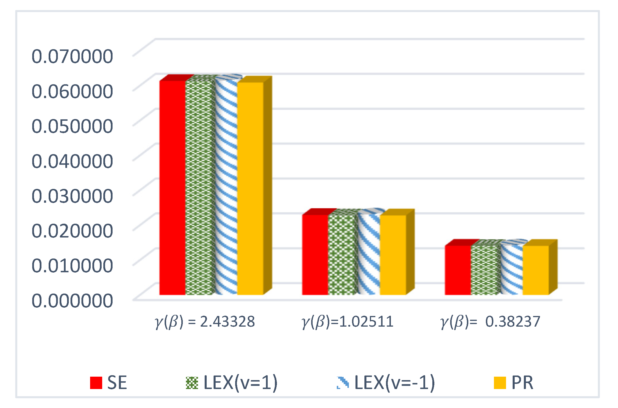
- We can see from Figure 1 that the estimated risk for at the true value for n = 30 has the lowest values when compared to the other estimates, except at the true value of
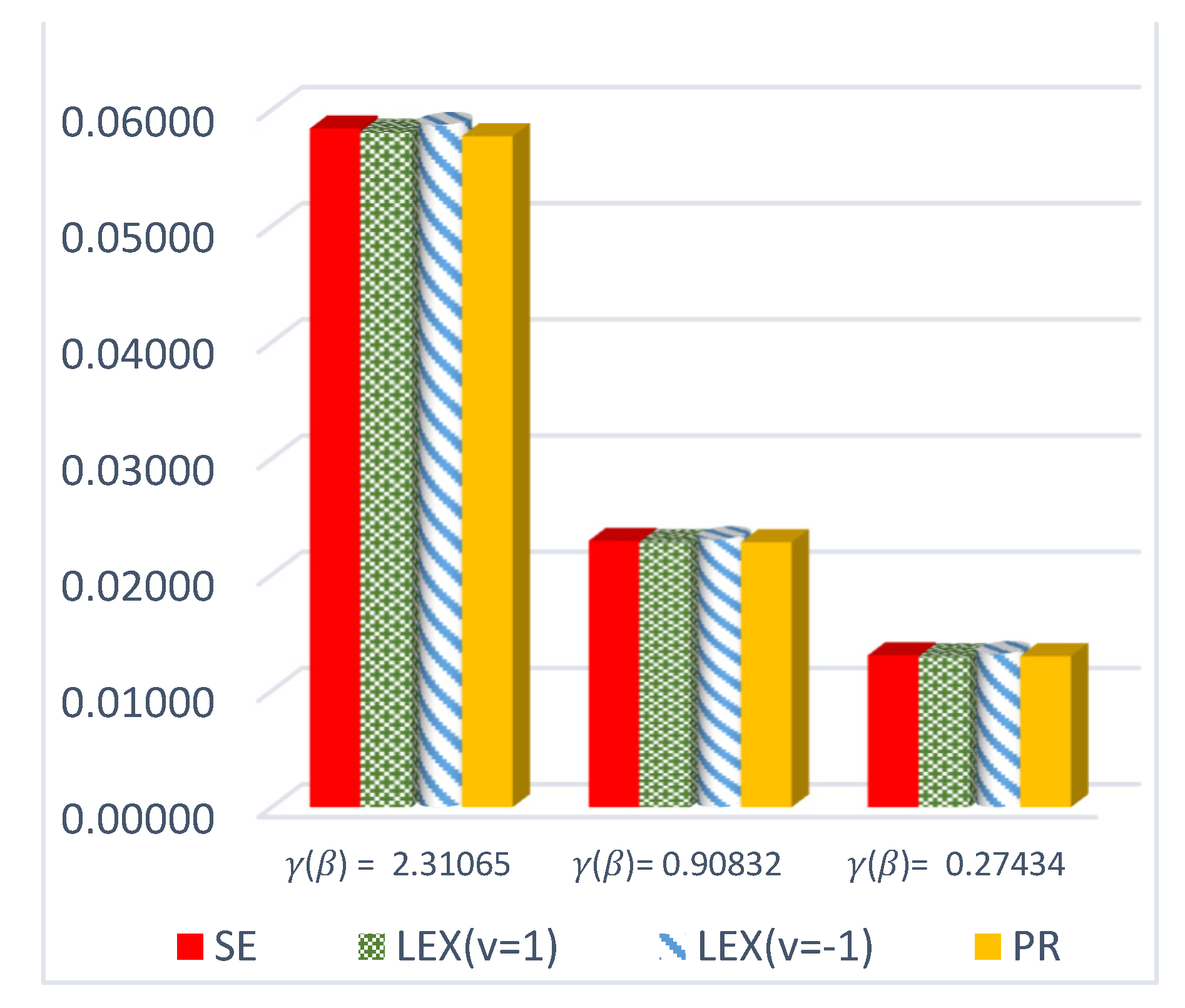
- Figure 2 indicates that the estimated risks of at v = 1 have the lowest value at when compared to the other estimates for n = 100.
The following are the notes that may be found at t = 1.5:
- The estimated risk of at v = −1 obtains the lowest values at n = 70 and 100 while the estimated risk of has the lowest values for n = 30 and 50. The width of the Bayesian credible interval for at v = −1 is the smallest in comparison with other estimates for n = 50 and 70 (see Table 4).
- At n = 30 and 100, the estimated risk of has the lowest values, while the estimated risk of has the lowest values at n = 50 and 70. The width of the Bayesian credible interval for at v = 1 is the shortest compared to the others via the SE and PR loss functions, except at n = 100 (see Table 5).
- We can see from Figure 3 that the estimated risk of at n = 30 holds the lowest values for all actual values of , except at
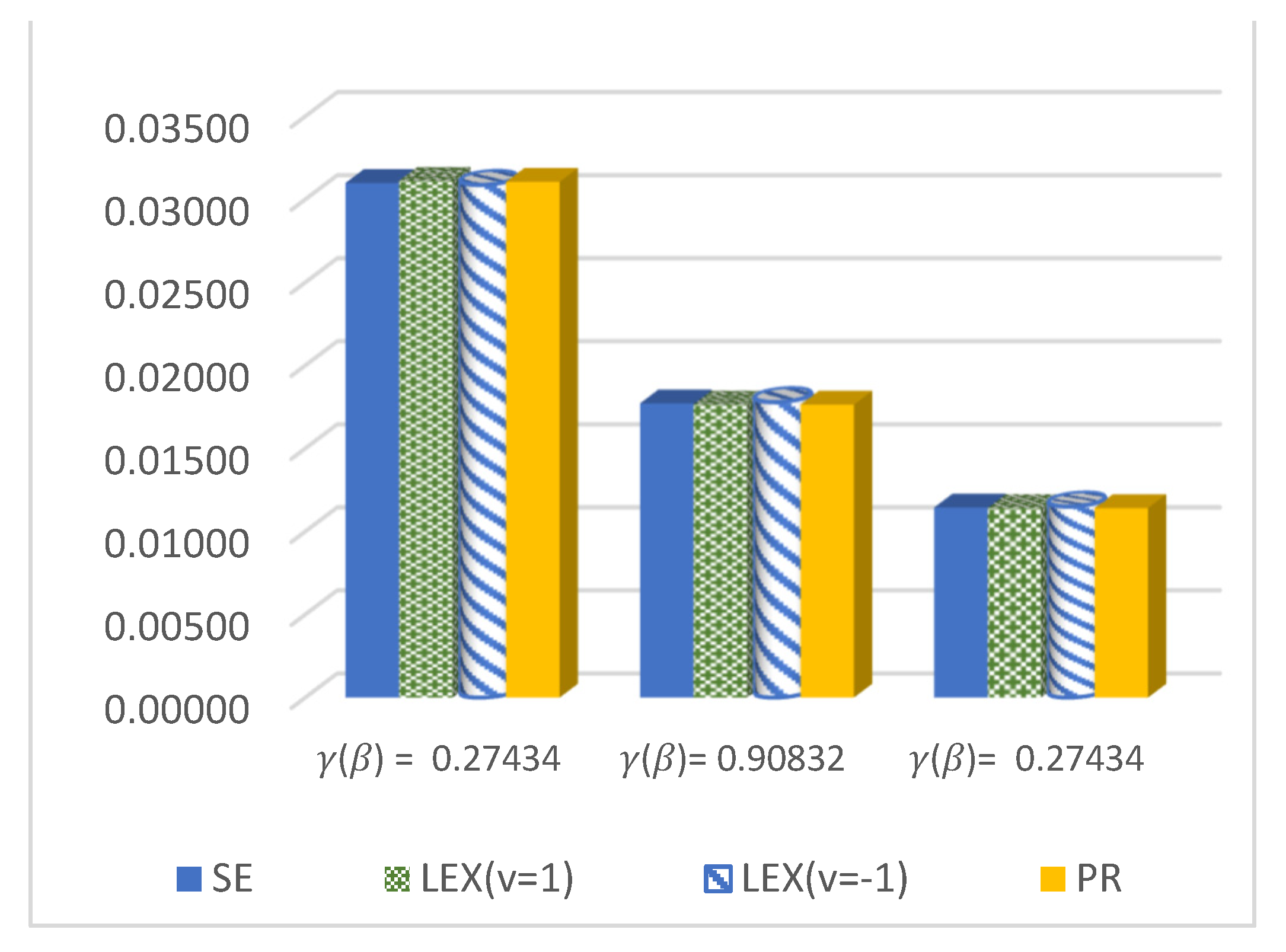
- For a large sample size (n = 100), the estimated risks for at v = 1 obtain the lowest value at actual value of , as shown in Figure 4.
- We conclude from Table 6 that the estimated risks of at v = 1 provide the lowest values for all values of n. Moreover, the width of the Bayesian credible intervals for at v = 1 takes the lowest values with respect to all possible values of n, except at n = 30 and 70.
4.2. Application
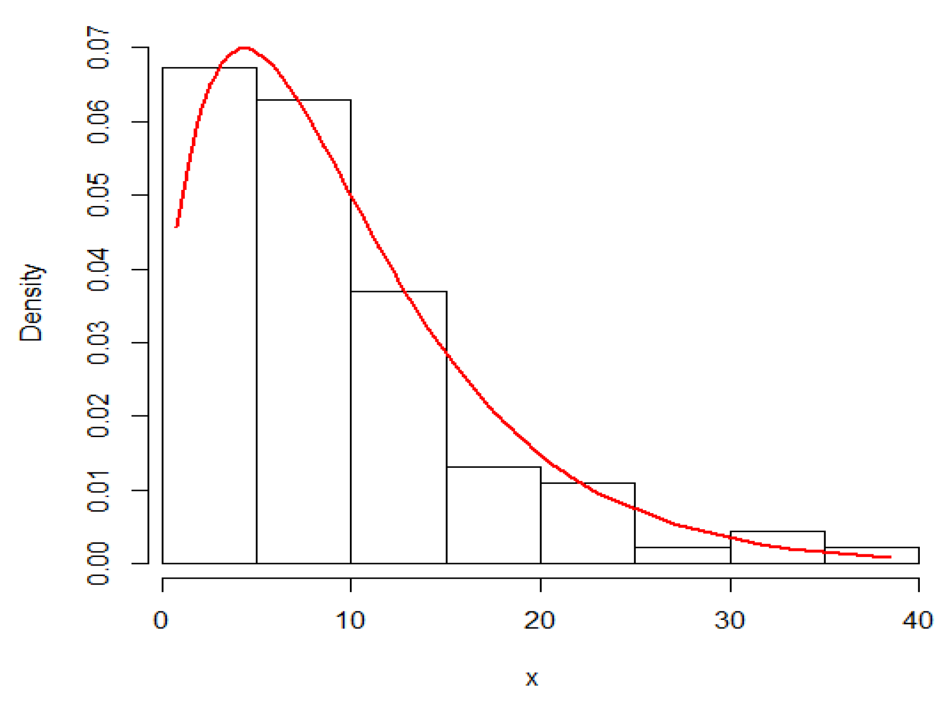
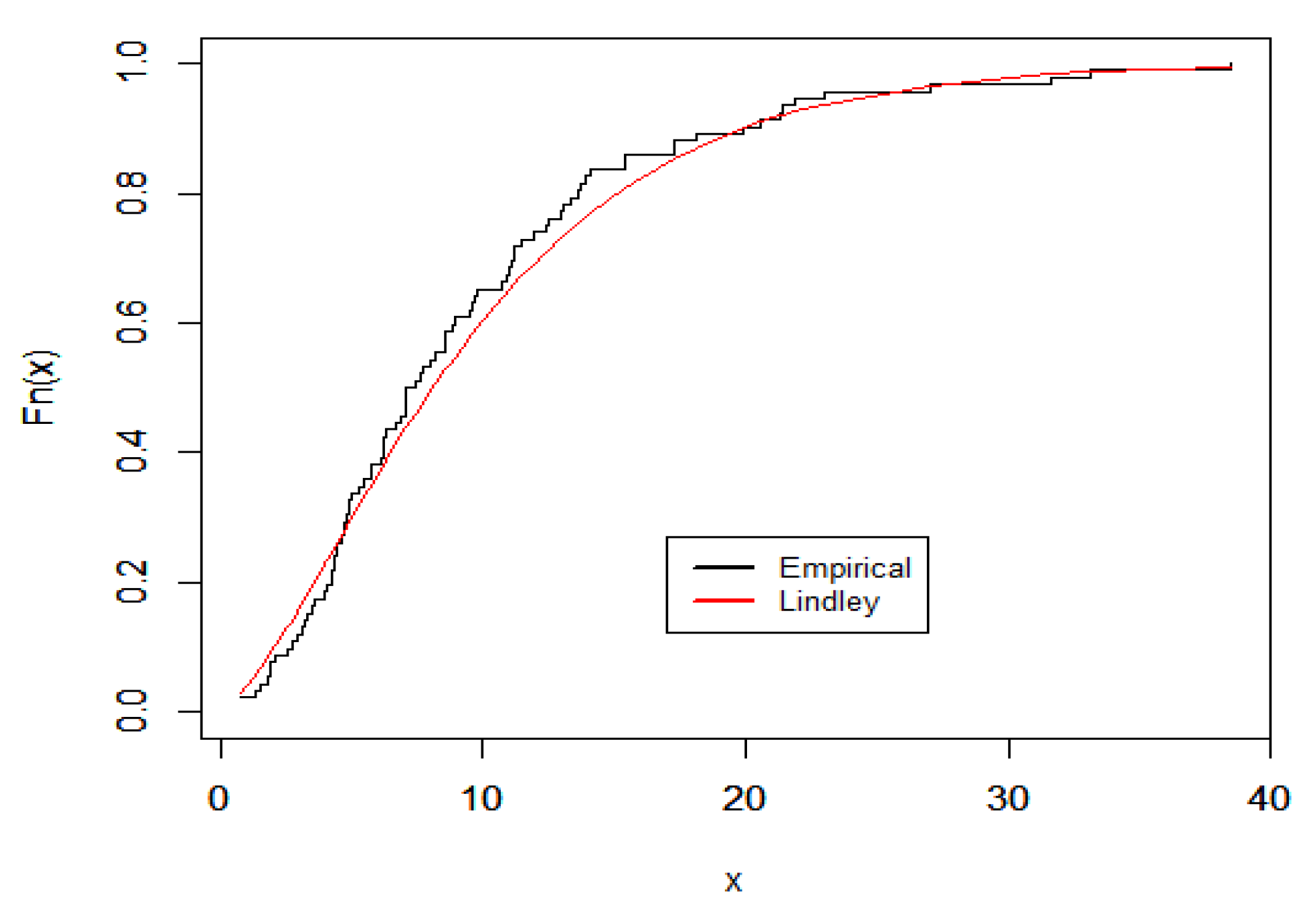
Here, we demonstrate the technique described in the preceding section by using an actual data set that represents the waiting times (in minutes) before receiving service for 100 bank customers. Reference [23] discussed the detailed statistics that showed the data fitted the Lindley distribution. Figure 8 and Figure 9 provide plots of fitted PDF and CDF for the data under consideration. The Bayes estimates of the DCRRéE at t = 0.5 and 1.5 at the intended loss functions are reported in Table 7.
As expected, the DCRRéE estimators for the proposed loss functions decrease with time, as seen in this example.
5. Concluding Remarks
The Bayesian estimators of the DCRRéE for the Lindley distribution are investigated in this study. The Bayesian estimators of the DCRRéE for the Lindley model are thought to be produced by both symmetric and asymmetric loss functions. The MCMoC method is used to calculate the Bayesian estimator and the Bayesian credible intervals. The behavior of the DCRRéE estimators for the Lindley distribution is evaluated using some precision criteria. Real-world data and simulation concerns are addressed. Regarding the outcomes of the study, we conclude that for small actual values of the DCRRéE, the estimated risk and width of the Bayesian credible intervals of the DCRRéE estimates under the linear exponential loss function are often fewer than those based on the squared error and precautionary loss functions. At t = 0.5, the width of the Bayesian credible intervals for the DCRRéE estimates via the linear exponential loss function is less than the others via the squared error and precautionary loss functions for a sample size of large values and large actual values of the DCRRéE. However, at t = 1.5, the width of the Bayesian credible interval for the DCRRéE estimates via the precautionary loss function is smaller than the equivalent estimates via the squared error and linear exponential loss functions. For small DCRRéE values, the Bayesian estimates via the linear exponential loss function are preferable to other estimates under the squared error and precautionary loss functions. However, for a high true value of the DCRRéE, the Bayesian estimates under the precautionary loss function are preferable to the other estimates via the loss functions chosen.
Author Contributions
Methodology, A.M.A., A.A., A.S.H., A.N.Z. and M.E. Conceptualization, A.S.H.; Data curation, A.M.A.; Funding acquisition, A.M.A.; Methodology, A.A.; Project administration, M.E.; Software, A.N.Z.; Supervision, M.E. All authors have read and agreed to the published version of the manuscript.
Funding
The Deanship of Scientific Research (DSR), King Abdul-Aziz University, Jeddah, supported this work under grant no. (KEP-PhD-69-130-42). The authors, therefore, gratefully acknowledge the technical and financial support of the DSR.
Institutional Review Board Statement
Not applicable.
Informed Consent Statement
Not applicable.
Data Availability Statement
If you would like to obtain the numerical dataset used to conduct the study reported in the publication, please contact the appropriate author.
Acknowledgement:
We would like to express our gratitude to the two reviewers for their insightfuland useful suggestions on this manuscript, which significantly enhanced it. This project was funded by the Deanship of Scientific Research (DSR), King Abdul-Aziz University, Jeddah, supported this work under grant no. (KEP-PhD-69-130-42). The authors, therefore, gratefully acknowledge the technical and financial support of the DSR.
Conflicts of Interest
The authors declare no conflict of interest.
Acronyms & Abbreviations
| BEs | Bayes estimates |
| CDF | Cumulative distribution function |
| DCR | dynamic cumulative residual |
| DCRRéE | dynamic cumulative residual Rényi entropy |
| ER | Estimated Risk |
| LINEx | Linear exponential loss function |
| L | Lower credible limit |
| MCMoC | Markov Chain Monte Carlo |
| MH | Metropolis–Hastings |
| Probability density function | |
| PR | Precautionary loss function |
| RABs | Relative absolute biases |
| SE | Squared error loss function |
| SF | Survival function |
| U | Upper credible limit |
| WD | Width of credible intervals |
References
- Rényi, A. On measures of Entropy and Information. In Proceeding of the Fourth Berkeley Symposium on Mathematical Statistics and Probability; University of California Press: Berkeley, CA, USA, 1961; Volume 1, pp. 547–561. [Google Scholar]
- Renner, R.; Gisin, N.; Kraus, B. An information-theoretic security proof for quantum-key-distribution protocols. Phys. Rev. A 2005, 72, 1–18. [Google Scholar] [CrossRef] [Green Version]
- Lévay, P.; Nagy, S.; Pipek, J. Elementary formula for entanglement entropies of fermionic systems. Phys. Rev. A 2005, 72, 1–8. [Google Scholar] [CrossRef] [Green Version]
- Baratpour, S.; Ahmadi, J.; Arghami, N.R. Entropy properties of record statistics. Stat. Pap. 2007, 48, 197–213. [Google Scholar] [CrossRef]
- Abo-Eleneen, Z.A. The entropy of progressively censored samples. Entropy 2011, 13, 437–449. [Google Scholar] [CrossRef] [Green Version]
- Seo, J.I.; Lee, H.J.; Kan, S.B. Estimation for generalized half logistic distribution based on records. J. Korean Inf. Sci. Soc. 2012, 23, 1249–1257. [Google Scholar] [CrossRef] [Green Version]
- Cho, Y.; Sun, H.; Lee, K. Estimating the Entropy of a Weibull Distribution under Generalized Progressive Hybrid Censoring. Entropy 2015, 17, 102–122. [Google Scholar] [CrossRef] [Green Version]
- Lee, K. Estimation of entropy of the inverse Weibull distribution under generalized progressive hybrid censored data. J. Korean Inf. Sci. Soc. 2017, 28, 659–668. [Google Scholar]
- Chacko, M.; Asha, P.S. Estimation of entropy for generalized exponential distribution based on record values. J. Indian Soc. Probab. Stat. 2018, 19, 79–96. [Google Scholar] [CrossRef]
- Al-Babtain, A.A.; Elbatal, I.; Chesneau, C.; Elgarhy, M. Estimation of different types of entropies for the Kumaraswamy distribution. PLoS ONE 2021, 16, e0249027. [Google Scholar] [CrossRef] [PubMed]
- Hassan, A.S.; Zaky, A.N. Entropy Bayesian estimation for Lomax distribution based on record. Thail. Stat. 2021, 19, 96–115. [Google Scholar]
- Hassan, A.S.; Zaky, A.N. Estimation of entropy for inverse Weibull distribution under multiple censored data. J. Taibah Univ. Sci. 2019, 13, 331–337. [Google Scholar] [CrossRef] [Green Version]
- Rao, M.; Chen, Y.; Vemuri, B.C.; Wang, F. Cumulative residual entropy: A new measure of information. IEEE Trans. Inf. Theory 2004, 50, 1220–1228. [Google Scholar] [CrossRef]
- Sunoj, S.M.; Linu, M.N. Dynamic cumulative rsidual Rényi’s entropy. Statistics 2012, 46, 41–56. [Google Scholar] [CrossRef]
- Kamari, O. On dynamic cumulative residual entropy of order statistics. J. Stat. Appl. Prob. 2016, 5, 515–519. [Google Scholar] [CrossRef]
- Kundu, C.; Crescenzo, A.D.; Longobardi, M. On cumulative residual (past) inaccuracy for truncated random variables. Metrika 2016, 79, 335–356. [Google Scholar] [CrossRef]
- Renjini, K.R.; Abdul-Sathar, E.I.; Rajesh, G. Bayes Estimation of Dynamic Cumulative Residual Entropy for Pareto Distribution Under Type-II Right Censored Data. Appl. Math. Model. 2016, 40, 8424–8434. [Google Scholar] [CrossRef]
- Renjini, K.R.; Abdul-Sathar, E.I.; Rajesh, G. A study of the effect of loss functions on the Bayes estimates of dynamic cumulative residual entropy for Pareto distribution under upper record values. J. Stat. Comput. Simul. 2016, 86, 324–339. [Google Scholar] [CrossRef]
- Renjini, K.R.; Abdul-Sathar, E.I.; Rajesh, G. Bayesian estimation of dynamic cumulative residual entropy for classical Pareto distribution. Am. J. Math. 2018, 37, 1–13. [Google Scholar] [CrossRef]
- Ahmadini, A.A.H.; Hassan, A.S.; Zaki, A.N.; Alshqaq, S.S. Bayesian Inference of Dynamic Cumulative Residual Entropy from Parto II distribution with Application to COVID-19. AIM Math. 2020, 6, 2196–2216. [Google Scholar] [CrossRef]
- Al-Babtain, A.A.; Hassan, A.S.; Zaky, A.N.; Elbatal, I.; Elgarhy, M. Dynamic cumulative residual Rényi entropy for Lomax distribution: Bayesian and non-Bayesian methods. AIM Math. 2021, 6, 3889–3914. [Google Scholar] [CrossRef]
- Lindley, D.V. Fiducial distributions and Bayes’ theorem. J. R. Stat. Soc. B 1958, 20, 102–107. [Google Scholar] [CrossRef]
- Ghitany, M.E.; Atieh, B.; Nadarajah, S. Lindley distribution and its application. Math. Comput. Simul. 2008, 78, 493–506. [Google Scholar] [CrossRef]
- Ghitany, M.E.; Alqallaf, F.; Al-Mutairi, D.K.; Husain, H.A. A two-parameter Lindley distribution and its applications to survival data. Math. Comput. Simul. 2011, 81, 1190–1201. [Google Scholar] [CrossRef]
- Ali, S.; Aslam, M.; Kazmi, S.M.A. A study of the effect of the loss function on Bayes Estimate, posterior risk and hazard function for Lindley distribution. Appl. Math. Model. 2013, 37, 6068–6078. [Google Scholar] [CrossRef]
- Al-Mutairi, D.K.; Ghitany, M.E.; Kundu, D. Inferences on stress-strength reliability from Lindley distributions. Commun. Stat. Theory Methods 2013, 42, 1443–1463. [Google Scholar] [CrossRef]
- Krishna, H.; Kumar, K. Reliability estimation in Lindley distribution with progressively type II right censored sample. Math. Comput. Simul. 2011, 82, 281–294. [Google Scholar] [CrossRef]
- Sharma, V.K.; Singh, S.K.; Singh, U.; Ul-Farhat, K. Bayesian estimation on interval censored Lindley distribution using Lindley’s approximation. Int. J. Syst. Assur. Eng. Manag. 2016, 8, 799–810. [Google Scholar] [CrossRef]
- Maiti, S.S.; Mukherjee, I. On estimation of the PDF and CDF of the Lindley distribution. Commun. Stat. Simul. Comput. 2018, 47, 1370–1381. [Google Scholar] [CrossRef]
- Hafez, E.H.; Riad, F.H.; Mubarak, S.A.M.; Mohamed, M.S. Study on Lindley distribution accelerated life tests: Application and numerical simulation. Symmetry 2020, 12, 2080. [Google Scholar] [CrossRef]
- Chen, M.H.; Shao, Q.M. Monte Carlo Estimation of Bayesian Credible and HPD Intervals. J. Comput. Graph. Stat. 1999, 8, 69–92. [Google Scholar]
- Metropolis, N.; Rosenbluth, A.W.; Rosenbluth, M.N.; Teller, A.H.; Teller, E. Equations of state calculations by fast computing machines. J. Chem. Phys. 1953, 21, 1087–1091. [Google Scholar] [CrossRef] [Green Version]
Figure 1.
ER of DCRRéE estimates under proposed loss functions at n = 30 and t = 0.5.

Figure 2.
ER of DCRRéE estimates under proposed loss functions at n = 100 and t = 0.5.

Figure 3.
ER of DCRRéE estimates under proposed loss functions at n = 30 and t = 1.5.

Figure 4.
ER of DCRRéE estimates under proposed loss functions at n = 100 and t = 1.5.

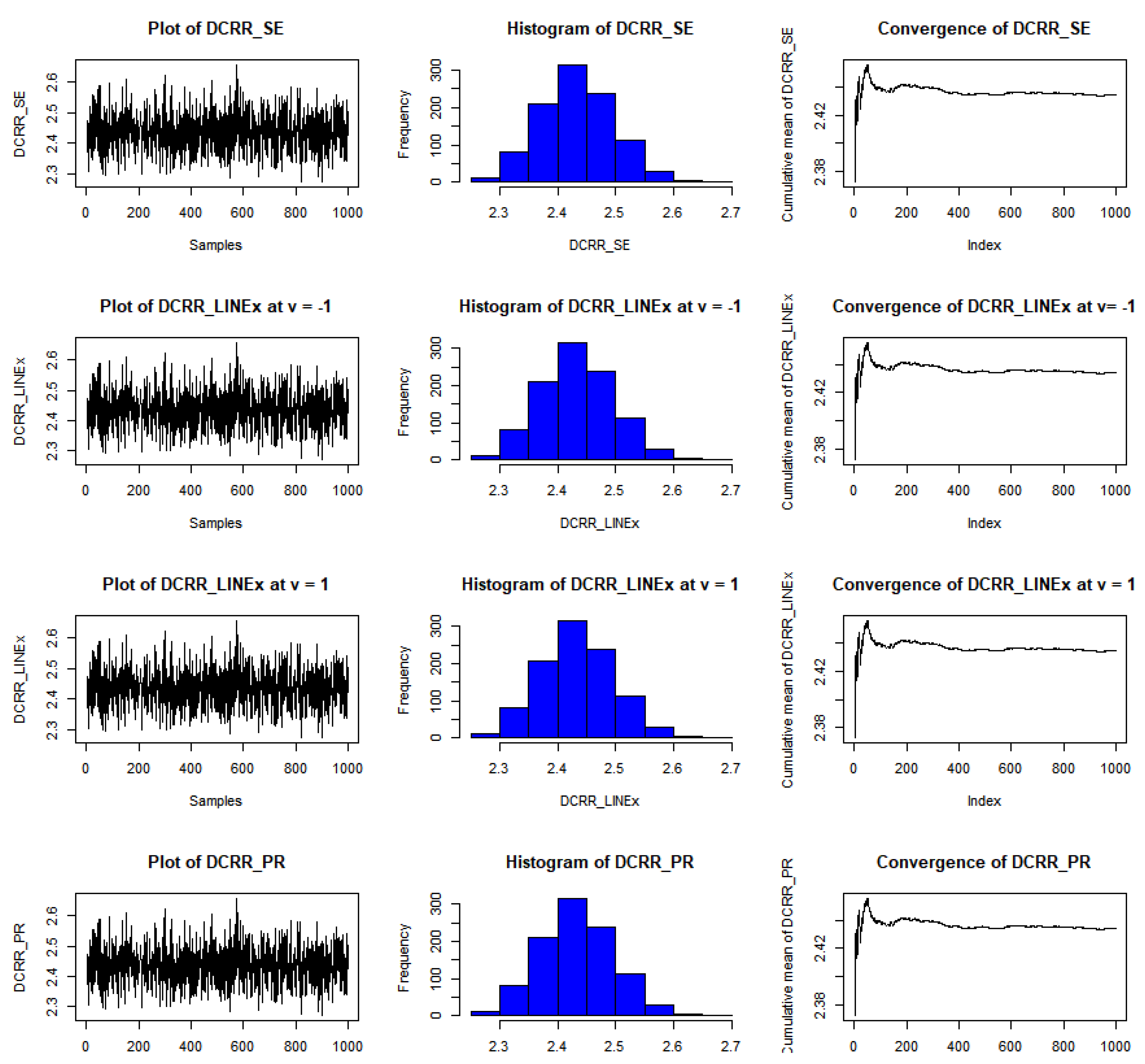
Figure 5.
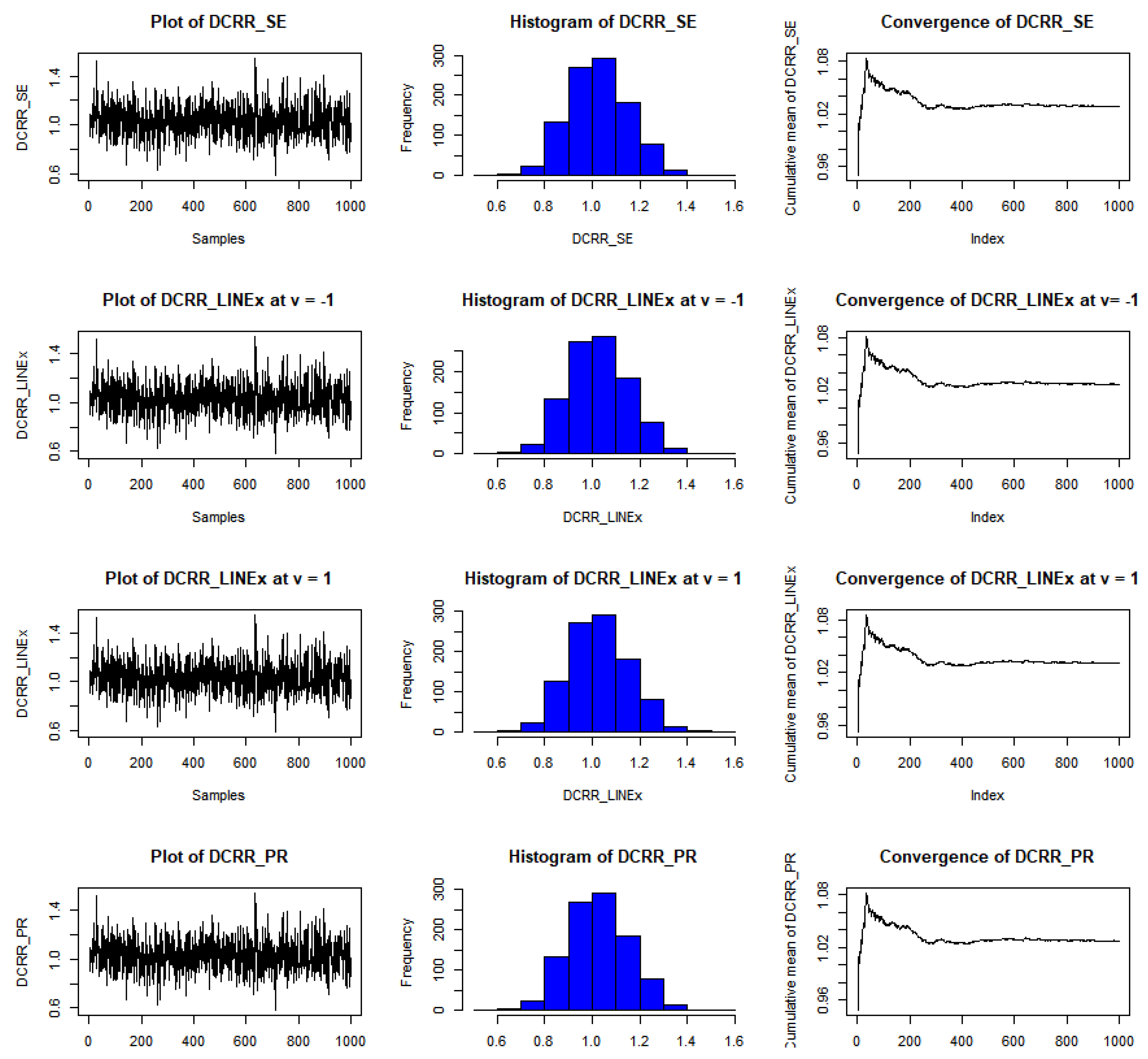
Example of convergence of MCMoC of estimates for , at t = 0.5, θ = 0.8, and n = 30.

Figure 6.
Example of convergence of MCMoC estimates for , at t = 0.5, θ = 1.5, and n = 100.

Figure 7.
Example of convergence of MCMoC estimates for , at t = 0.5, θ = 2.0, and n = 50.

Figure 8.
Fitted PDF plots of Lindley model for the data set.

Figure 9.
Fitted CDF plots of Lindley model for the data set.


Table 1.
Measures of Accuracy for DCRRéE at , and .
| n | SE | LINEx (v = 1) | LINEx (v = −1) | PR | ||||||||||||
|---|---|---|---|---|---|---|---|---|---|---|---|---|---|---|---|---|
| BE | RAB | ER | WD | BE | RAB | ER | WD | BE | RAB | ER | WD | BE | RAB | ER | WD | |
| 30 | 2.42926 | 0.00166 | 0.06132 | 0.94796 | 2.42550 | 0.00320 | 0.06121 | 0.94596 | 2.43302 | 0.00011 | 0.06146 | 0.95129 | 2.42450 | 0.00361 | 0.06088 | 0.94389 |
| 50 | 2.42149 | 0.00485 | 0.04538 | 0.78382 | 2.41824 | 0.00618 | 0.04552 | 0.78713 | 2.42475 | 0.00351 | 0.04528 | 0.78514 | 2.41744 | 0.00651 | 0.04537 | 0.78679 |
| 70 | 2.41950 | 0.00567 | 0.03941 | 0.75725 | 2.41658 | 0.00687 | 0.03951 | 0.75845 | 2.42242 | 0.00447 | 0.03934 | 0.75966 | 2.41587 | 0.00716 | 0.03939 | 0.75794 |
| 100 | 2.43023 | 0.00126 | 0.02889 | 0.66839 | 2.42763 | 0.00233 | 0.02894 | 0.66955 | 2.43284 | 0.00018 | 0.02885 | 0.66541 | 2.42699 | 0.00259 | 0.02887 | 0.66919 |
Table 2.
Measures of Accuracy for DCRRéE at , and .
| n | SE | LINEx (v = 1) | LINEx (v = −1) | PR | ||||||||||||
|---|---|---|---|---|---|---|---|---|---|---|---|---|---|---|---|---|
| BE | RAB | ER | WD | BE | RAB | ER | WD | BE | RAB | ER | WD | BE | RAB | ER | WD | |
| 30 | 1.02767 | 0.00250 | 0.02292 | 0.59123 | 1.02535 | 0.00023 | 0.022793 | 0.59016 | 1.03000 | 0.00477 | 0.02306 | 0.59175 | 1.02610 | 0.00096 | 0.022787 | 0.59015 |
| 50 | 1.03075 | 0.00550 | 0.02128 | 0.56636 | 1.02856 | 0.00336 | 0.02123 | 0.56555 | 1.03295 | 0.00764 | 0.02135 | 0.56662 | 1.02928 | 0.00406 | 0.02121 | 0.56545 |
| 70 | 1.01934 | 0.00563 | 0.02024 | 0.54244 | 1.01716 | 0.00776 | 0.02025 | 0.53970 | 1.02153 | 0.00350 | 0.02025 | 0.54470 | 1.01788 | 0.00706 | 0.02021 | 0.54031 |
| 100 | 1.02838 | 0.00319 | 0.01682 | 0.48992 | 1.02636 | 0.00121 | 0.01676 | 0.49011 | 1.03041 | 0.00516 | 0.01689 | 0.49149 | 1.02702 | 0.00186 | 0.01675 | 0.48942 |
Table 3.
Measures of Accuracy for DCRRéE for , and .
| n | SE | LINEx (v = 1) | LINEx (v = − 1) | PR | ||||||||||||
|---|---|---|---|---|---|---|---|---|---|---|---|---|---|---|---|---|
| BE | RAB | ER | WD | BE | RAB | ER | WD | BE | RAB | ER | WD | BE | RAB | ER | WD | |
| 30 | 0.39342 | 0.02888 | 0.01409 | 0.45858 | 0.39158 | 0.02408 | 0.01403 | 0.45810 | 0.39525 | 0.03368 | 0.01415 | 0.45534 | 0.39249 | 0.02646 | 0.01404 | 0.45710 |
| 50 | 0.38557 | 0.00835 | 0.01334 | 0.43146 | 0.38381 | 0.00377 | 0.01330 | 0.43208 | 0.38732 | 0.01294 | 0.01339 | 0.43187 | 0.38468 | 0.00604 | 0.01331 | 0.43033 |
| 70 | 0.38513 | 0.00721 | 0.01254 | 0.42933 | 0.38347 | 0.00287 | 0.01252 | 0.42705 | 0.38679 | 0.01156 | 0.01257 | 0.42750 | 0.38429 | 0.00503 | 0.01257 | 0.42820 |
| 100 | 0.38601 | 0.00952 | 0.01141 | 0.41235 | 0.38437 | 0.00522 | 0.01140 | 0.41399 | 0.38766 | 0.01383 | 0.01142 | 0.41399 | 0.38519 | 0.00736 | 0.01139 | 0.41346 |
Table 4.
Measures of Accuracy for DCRRéE for , and .
| n | SE | LINEx (v = 1) | LINEx (v = −1) | PR | ||||||||||||
|---|---|---|---|---|---|---|---|---|---|---|---|---|---|---|---|---|
| BE | RAB | ER | WD | BE | RAB | ER | WD | BE | RAB | ER | WD | BE | RAB | ER | WD | |
| 30 | 2.34019 | 0.01279 | 0.05839 | 0.92243 | 2.33632 | 0.01111 | 0.05811 | 0.92058 | 2.34407 | 0.01446 | 0.05871 | 0.91961 | 2.33524 | 0.01064 | 0.05774 | 0.91789 |
| 50 | 2.29427 | 0.00709 | 0.04883 | 0.86754 | 2.29102 | 0.00850 | 0.04888 | 0.86787 | 2.29753 | 0.00568 | 0.04880 | 0.86563 | 2.29020 | 0.00885 | 0.04869 | 0.86675 |
| 70 | 2.29300 | 0.00764 | 0.03709 | 0.74947 | 2.29013 | 0.00888 | 0.03725 | 0.75022 | 2.29586 | 0.00640 | 0.03695 | 0.74925 | 2.28945 | 0.00918 | 0.03717 | 0.74970 |
| 100 | 2.28540 | 0.01093 | 0.03098 | 0.65564 | 2.28284 | 0.01204 | 0.03112 | 0.65423 | 2.28797 | 0.00982 | 0.03087 | 0.65897 | 2.28222 | 0.01230 | 0.03106 | 0.65275 |
Table 5.
Measures of Accuracy for DCRRéE for , and .
| n | SE | LINEx (v = 1) | LINEx (v = −1) | PR | ||||||||||||
|---|---|---|---|---|---|---|---|---|---|---|---|---|---|---|---|---|
| BE | RAB | ER | WD | BE | RAB | ER | WD | BE | RAB | ER | WD | BE | RAB | ER | WD | |
| 30 | 0.91976 | 0.01260 | 0.02292 | 0.56958 | 0.91744 | 0.01005 | 0.022792 | 0.56538 | 0.92208 | 0.01515 | 0.02306 | 0.57188 | 0.91819 | 0.01087 | 0.022788 | 0.56644 |
| 50 | 0.91339 | 0.00559 | 0.02011 | 0.54160 | 0.91124 | 0.00322 | 0.02092 | 0.53828 | 0.91555 | 0.00796 | 0.02021 | 0.54329 | 0.91194 | 0.00399 | 0.02091 | 0.55795 |
| 70 | 0.89959 | 0.00961 | 0.02005 | 0.54054 | 0.89749 | 0.01192 | 0.02081 | 0.53003 | 0.90169 | 0.00730 | 0.02011 | 0.53211 | 0.89820 | 0.01114 | 0.02076 | 0.54979 |
| 100 | 0.91480 | 0.00714 | 0.01771 | 0.51330 | 0.91285 | 0.00499 | 0.01765 | 0.51441 | 0.91675 | 0.00928 | 0.01779 | 0.51429 | 0.91349 | 0.00569 | 0.01764 | 0.51315 |
Table 6.
Measures of Accuracy for DCRRéE at , and .
| n | SE | LINEx (v = 1) | LINEx (v = −1) | PR | ||||||||||||
|---|---|---|---|---|---|---|---|---|---|---|---|---|---|---|---|---|
| BE | RAB | ER | WD | BE | RAB | ER | WD | BE | RAB | ER | WD | BE | RAB | ER | WD | |
| 30 | 0.28367 | 0.03401 | 0.01306 | 0.43538 | 0.28192 | 0.02763 | 0.01296 | 0.43471 | 0.28542 | 0.04039 | 0.01318 | 0.43649 | 0.28278 | 0.03077 | 0.01300 | 0.43461 |
| 50 | 0.27769 | 0.01221 | 0.01285 | 0.43401 | 0.27596 | 0.00591 | 0.012817 | 0.43286 | 0.27942 | 0.01853 | 0.01290 | 0.43440 | 0.27682 | 0.00903 | 0.01282 | 0.43410 |
| 70 | 0.28249 | 0.02972 | 0.01277 | 0.43031 | 0.28072 | 0.02326 | 0.01272 | 0.43063 | 0.28427 | 0.03620 | 0.01283 | 0.42760 | 0.28160 | 0.02646 | 0.01273 | 0.43075 |
| 100 | 0.28390 | 0.03486 | 0.01145 | 0.41154 | 0.28225 | 0.02883 | 0.01140 | 0.40894 | 0.28556 | 0.04089 | 0.01150 | 0.41205 | 0.28307 | 0.03182 | 0.01141 | 0.41037 |
Table 7.
DCRRéE Bayesian estimates at t = 0.5 and 1.5 for elected loss functions.
| t | ||||
|---|---|---|---|---|
| 0.5 | 3.711552 | 3.701186 | 3.703288 | 3.708402 |
| 1.5 | 3.638074 | 3.634769 | 3.638159 | 3.635013 |
Publisher’s Note: MDPI stays neutral with regard to jurisdictional claims in published maps and institutional affiliations. |
© 2021 by the authors. Licensee MDPI, Basel, Switzerland. This article is an open access article distributed under the terms and conditions of the Creative Commons Attribution (CC BY) license (https://creativecommons.org/licenses/by/4.0/).
Share and Cite
MDPI and ACS Style
Almarashi, A.M.; Algarni, A.; Hassan, A.S.; Zaky, A.N.; Elgarhy, M. Bayesian Analysis of Dynamic Cumulative Residual Entropy for Lindley Distribution. Entropy 2021, 23, 1256. https://0-doi-org.brum.beds.ac.uk/10.3390/e23101256
AMA Style
Almarashi AM, Algarni A, Hassan AS, Zaky AN, Elgarhy M. Bayesian Analysis of Dynamic Cumulative Residual Entropy for Lindley Distribution. Entropy. 2021; 23(10):1256. https://0-doi-org.brum.beds.ac.uk/10.3390/e23101256
Chicago/Turabian StyleAlmarashi, Abdullah M., Ali Algarni, Amal S. Hassan, Ahmed N. Zaky, and Mohammed Elgarhy. 2021. "Bayesian Analysis of Dynamic Cumulative Residual Entropy for Lindley Distribution" Entropy 23, no. 10: 1256. https://0-doi-org.brum.beds.ac.uk/10.3390/e23101256
Note that from the first issue of 2016, this journal uses article numbers instead of page numbers. See further details here.