
Enhanced Slime Mould Algorithm for Multilevel Thresholding Image Segmentation Using Entropy Measures


1
College of Marine Engineering, Dalian Maritime University, Dalian 116026, China
2
School of Information Engineering, Sanming University, Sanming 365004, China
3
Faculty of Computer Sciences and Informatics, Amman Arab University, Amman 11953, Jordan
4
School of Computer Science, Universiti Sains Malaysia, Pulau Pinang 11800, Malaysia
5
Department of Management Information System, College of Business Administration, Taif University, P.O. Box 11099, Taif 21944, Saudi Arabia
*
Authors to whom correspondence should be addressed.
Entropy 2021, 23(12), 1700; https://0-doi-org.brum.beds.ac.uk/10.3390/e23121700
Submission received: 18 November 2021
/
Revised: 17 December 2021
/
Accepted: 17 December 2021
/
Published: 20 December 2021
Abstract
:Image segmentation is a fundamental but essential step in image processing because it dramatically influences posterior image analysis. Multilevel thresholding image segmentation is one of the most popular image segmentation techniques, and many researchers have used meta-heuristic optimization algorithms (MAs) to determine the threshold values. However, MAs have some defects; for example, they are prone to stagnate in local optimal and slow convergence speed. This paper proposes an enhanced slime mould algorithm for global optimization and multilevel thresholding image segmentation, namely ESMA. First, the Levy flight method is used to improve the exploration ability of SMA. Second, quasi opposition-based learning is introduced to enhance the exploitation ability and balance the exploration and exploitation. Then, the superiority of the proposed work ESMA is confirmed concerning the 23 benchmark functions. Afterward, the ESMA is applied in multilevel thresholding image segmentation using minimum cross-entropy as the fitness function. We select eight greyscale images as the benchmark images for testing and compare them with the other classical and state-of-the-art algorithms. Meanwhile, the experimental metrics include the average fitness (mean), standard deviation (Std), peak signal to noise ratio (PSNR), structure similarity index (SSIM), feature similarity index (FSIM), and Wilcoxon rank-sum test, which is utilized to evaluate the quality of segmentation. Experimental results demonstrated that ESMA is superior to other algorithms and can provide higher segmentation accuracy.
1. Introduction
Image segmentation is fundamental and challenging work in computer vision, pattern recognition, and image processing. It is widely used in various fields, such as ship target segmentation and medical image processing [1]. The main goal of segmentation is to divide the image into homogeneous classes. The elements of each class share common attributes such as grayscale, feature, color, intensity, or texture [2,3,4,5]. In the literature, there are four standard image segmentation methods, which can be divided into (1) clustering-based methods, (2) region-based methods, (3) graph-based methods, (4) thresholding-based methods. Among the existing methods, one of the most widespread techniques is multilevel thresholding, which is widely used owing to its ease of implementation, high performance, and robustness compared with other methods [6]. Image thresholding techniques can be classified into two categories: Bilevel and multilevel. In the prior category, the image is separated into two homogeneous foreground and background areas using a single threshold value. The latter segment-techniques segment divides an image into more than two regions based on pixel intensities known as histogram [7]. Bilevel thresholding can solve simple image segmentation problems involving only two grey levels. However, the bilevel cannot be suitable for complicated and high-grade images. Therefore, the multilevel thresholding technique is the primary method for real-world applications [8]. Generally speaking, selecting threshold values is crucial when segmenting an image because of the enormous image thresholds. Consequently, it is formulated into an optimization problem, which includes parametric or nonparametric methods [9].
The parametric approach considers that each image class can be defined using probability density distributions, but this technique is computationally expensive. By contrast, the nonparametric approach uses criteria to separate the pixels into homogeneous regions, and then the thresholds are determined using statistical measures (entropy or variance) [10]. Over the years, many works in the literature have proposed some of these criteria. Among them, Otsu’s technique maximizes the between-class variance of each segmented class to achieve the optimal thresholds [11]. Kapur’s approach used the entropy of the histogram as a formula to obtain the optimal thresholds [12]. Li et al. [13] presented the minimum cross-entropy to minimize the cross-entropy between the original and segmented image to get the optimal thresholds values.
Notwithstanding, these approaches have limitations; for example, they are computationally expensive, significantly when the number of thresholds is increased. Therefore, multilevel thresholding is considered a particular challenge that needs to be optimized. For these reasons, meta-heuristic methods are commonly utilized in the related literature to solve these problems [14].
MAs are inspired by nature, including areas such as physics, biology, and social behavior. Owing to their easy implementation, flexibility, and high performance, many scholars have used them to determine the optimal values for real-world problems [15,16,17,18,19,20]. Over the past years, many meta-heuristic algorithms have been proposed. For instance, Particle Swarm Optimization (PSO) [21], Differential Evolution (DE) [22], Genetic Algorithm [23], Teaching-Learning-based Optimization (TLBO) [24], Simulated Annealing (SA) [25], Gravity Search Algorithm (GSA) [26], and Ant Colony Optimization Algorithm (ACO) [27]. Other than these classic algorithms, many novel MAs have been proposed in the literature and widely used in different domains, such as Gray Wolf Optimization (GWO) [28], Whale Optimization Algorithm (WOA) [29], Salp Swarm Algorithm (SSA) [30], Sine Cosine Algorithm (SCA) [31], Arithmetic Optimization Algorithm (AOA) [32], Aquila Optimizer (AO) [33], Multi-Verse Optimization (MVO) [34], Slime Mould Algorithm (SMA) [35], and Remora Optimization Algorithm (ROA) [36].
In the literature, many works show the efficiency of MAs in obtaining optimal thresholds; the following are a few outstanding research works. Jia et al. [37] proposed an improved moth-flame optimization for color image segmentation using Otsu’s between-class variance and Kapur’s entropy as objective functions. The proposed method was compared with FPA, ACO, PSO, etc. Wu et al. [38] presented an ameliorated teaching-learning-based optimization based on a random learning method for multilevel thresholding using Kapur’s entropy and Otsu’s between-class variance. Pare et al. [39] proposed a color image multilevel segmentation strategy based on the Bat algorithm and Renyi’s entropy as the criterion to tackle the problems of multi-thresholding. Zhao et al. [40] presented a variant of SMA based on diffusion mechanism and association strategy for CT image segmentation. In this work, Renyi’s entropy was the objective fitness function. All of these works are examples of meta-heuristic algorithms applied in multilevel thresholding image segmentation. Generally, they provide good results on some benchmark images. However, considering the No Free Lunch (NFL) theorem proposed by Wolpert in 1997 [41], no unique optimization algorithm is available for solving all optimization problems. Furthermore, all meta-heuristic algorithms have limitations that affect the optimization capability, such as showing low convergence speed and unbalancing the exploration and exploitation ability.
Slime mould algorithm (SMA) is a novel meta-heuristic algorithm proposed by Li et al. in 2020 [35], which is inspired by the oscillation mode and behavior of slime mould in foraging. Since SMA has few parameters and shows better performance in specific fields, many scholars utilize it to solve questions of reality, such as parameter optimization of the fuzzy system and feature selection [36,37]. However, similar to other MAs, SMA may fall into local optimal and slow convergence speed in some optimization problems. Thus, many contributed works are proposed to enhance the performance of SMA. Dhawale et al. [42] suggested an improved SMA based on a chaotic strategy for solving global optimization and constrained engineering problems. Mostafa et al. [43] presented a modified SMA by adaptive weight to estimate the PV panel parameters. Hassan et al. [44] proposed an improved SMA via sine and cosine operators for solving economic and emission dispatch problems. Ewees et al. [45] integrated the SMA and firefly algorithm to improve the performance for feature selection.
While these proposed improved versions of the SMA algorithm are better than the original SMA algorithm on specific problems, when solving multilevel thresholding image segmentation, the imbalance between exploration and exploitation is still an unavoidable problem. This paper proposes a novel variant of SMA (ESMA) with the Levy flight and quasi opposition-based learning to tackle these shortcomings and obtain high-quality threshold values in image segmentation. The improvement involves two primary approaches. Firstly, the Levy flight strategy is applied to improve the exploration capability of SMA. Moreover, a novel variant of opposition-based learning (OBL), called quasi opposition-based learning (QOBL), is utilized to improve the ability to jump out the local optimal and balance the exploration and exploitation. In the experimental phase, the proposed ESMA is then tested on the 23 benchmark functions and applied to solve the multilevel thresholding image segmentation problem.
Meanwhile, the ESMA is also used to compare with other MAs. Furthermore, for the field of image segmentation, we evaluated the image segmentation results using Peak Signal to Noise Ratio (PSNR), Structural Similarity Index (SSIM), and Feature Similarity Index (FSIM). The experimental results illustrate that the proposed algorithm can produce high-quality results for benchmark functions and the image segmentation field.
Specifically, the main contributions of this paper can be summarized as follows:
- ESMA based on Levy flight and quasi opposition-based learning for solving global optimization problems and multilevel thresholding image segmentation.
- The optimization performance of ESMA is evaluated on 23 benchmark functions including unimodal and multimodal.
- DSMA is applied for thresholding segmentation using minimum cross-entropy measure.
- The segmentation quality is verified according to the PSNR, SSIM, FSIM, and statistical test.
- The performance of DSMA is compared with several classical and state-of-the-art optimization algorithm.
The remainder of this paper can be organized as follows: Section 2 describes a brief overview of SMA, Levy flight, quasi opposition-based learning, and maximum cross-entropy measure. Section 3 provides the details of the proposed algorithm. The experimental results are discussed and analyzed in detail in Section 4 and Section 5. Finally, the conclusion and future work are discussed in Section 6.
2. Preliminaries
This section presents the main inspiration and mathematical model of the slime mould algorithm (SMA). Next, the improvement strategy including Levy flight, and quasi opposition-based learning will be described. Finally, we will describe the minimum cross-entropy measure.
2.1. Slime Mould Algorithm
The slime mould algorithm (SMA) is a meta-heuristic optimization algorithm proposed recently by Li et al. [35], which is inspired by the oscillation behavior of slime mould in foraging. Slime mould achieves positive and negative feedback according to the quality of the food source. If the quality of the food source is high, the slime mould will use the region-limited search strategy. Meanwhile, if the food source is of low quality, the slime mould will leave this area and move to another food source in search space. Furthermore, SMA also has a slight chance of z to reinitialize the population in the search space.
Based on the above description, the updating process of slime mould can be expressed as in the following equation:
where z denotes the probability of slime mould reinitializing, which is 0.03; r1, r2, and r3 denote the random value in [0,1]; LB and UB represent the lower and upper bound of search space, respectively; t is the current iteration. represents global best solution; both and denote the random individual; ∈ [−a,a], and decreases linearly from one to zero. represents the weight of slime mould.
The p can be calculated as follows:
where i ∈ 1,2, …, N, S(i) is the sequence representing the fitness of search agents. DF indicates the best fitness obtained by the slime mould.
can be calculated as follows:
where T represents the maximum iteration.
Note that the coefficient is an essential parameter, which simulates the oscillation frequency of slime mould under different food sources. The can be calculated as follows:
where r4 is a random value in [0,1]; bF and wF represent the best fitness and worst fitness obtained currently, respectively; condition indicates the rank first half of the search agent of S(i). The pseudo-code of SMA is shown in Algorithm 1.
| Algorithm 1 Pseudo-code of SMA |
| Initialize the positions of search agent; |
| While current iteration < maximum iteration do |
| Check if any search agent goes beyond the search space and amend it; |
| Calculate the fitness of all slime mould; |
| For each search agent do |
| Update positions by Equation (1); |
| End For |
| t = t + 1; |
| End While |
| Return the best solution; |
2.2. Levy Flight
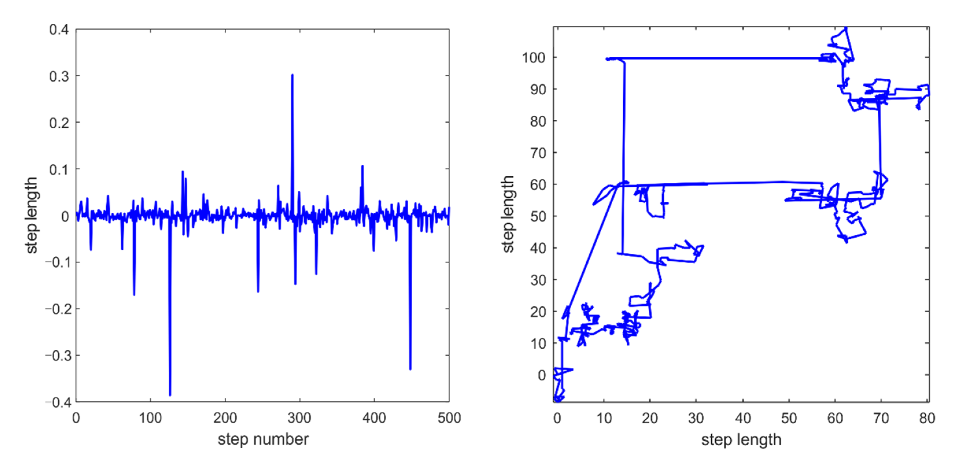
Numerous studies reveal that the flight trajectories of many flying animals are consistent with characteristics typical of Levy flight. Levy flight is a class of non-Gaussian random walk that follows Levy distribution [46,47]. It performs occasional long-distance walking with frequent short-distance steps, as shown in Figure 1. The mathematical formula for Levy flight is as follows:
where r4 and r5 are random values in [0,1], and β is a constant equal to 1.5.
2.3. Quasi Opposition-Based Learning
2.3.1. Opposition-Based Learning
Opposition-based learning (OBL) is an efficient search approach to avoid premature convergence, which was proposed by Tizhoosh in 2005 [48]. The main idea of OBL is to generate the opposite solution in the search space, then evaluate the original solution and its opposite solution by the objective function, respectively. Next, the best solution will be retained and go into the next iteration. Typically, the OBL strategy has high opportunities to provide closer optimal solutions than random ones.
We assume x to be an actual number in one dimension. Its opposite number xobl can be calculated by:
2.3.2. Quasi Opposition-Based Learning
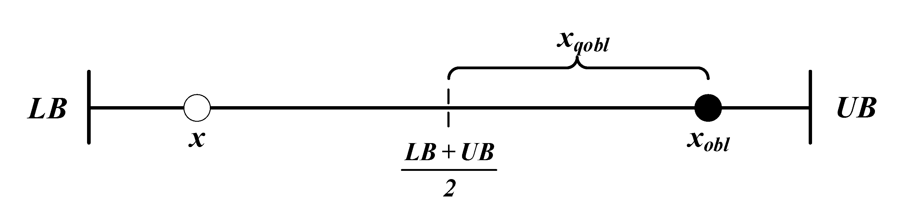
Based on the above description, a variant of OBL called quasi opposition-based learning (QOBL) was proposed by Rahnamayan et al. [49]. Unlike OBL, the QOBL strategy applied a quasi-opposite solution rather than the opposite solution. Therefore, the QOBL approach is more effective in finding globally optimal solutions than the previous strategy. On the basic theory of opposite solution, the quasi-opposite solution can be calculated by:
To understand the above theory more clearly, Figure 2 illustrates the original solution x, its opposite solution xobl, and its quasi-opposite solution xqobl.
2.4. Minimum Cross-Entropy
In 1968, cross-entropy was proposed by Kullback [50]. Cross-entropy measures the difference information between two probability distributions and , defined by:
In this work, we utilized minimum cross-entropy as a fitness function to find the optimal threshold value. The lower value of cross-entropy means less uncertainty and greater homogeneity. Let I be the origin grey image and h(i) be its histogram. Then, the thresholded image Ith can be calculated as follows:
where th denotes the threshold and divides the image into two different regions (foreground and background), and can be calculated by:
The cross-entropy can be computed by:
The above objective functions are utilized to calculate the threshold value for bilevel thresholding. Thus it can be extended to a multilevel strategy. Yin [51] proposed a faster technique to obtain the threshold values for the digital image. The formula is as follows:
where the above formula is based on thresholds , which contain nt different threshold values, by:
where nt represents the total number of thresholds and Hi can be defined as follows:
3. The Proposed Algorithm
3.1. Details of ESMA
The standard slime mould algorithm is a simple and efficient approach to solving specific optimization problems. However, based on the NFL theorem, no unique optimization algorithm is available for solving all optimization problems. Furthermore, SMA may be trapped into local optimal and show unperfected convergence speed for specific problems such as multilevel thresholding image segmentation. In order to improve the search ability and balance exploration and exploitation, in this paper, we propose an enhanced slime mould algorithm (ESMA) to improve the optimization performance. The improvement involves two major methods. Firstly, the Levy flight was used to enhance the exploration ability of SMA, which can be calculated by:
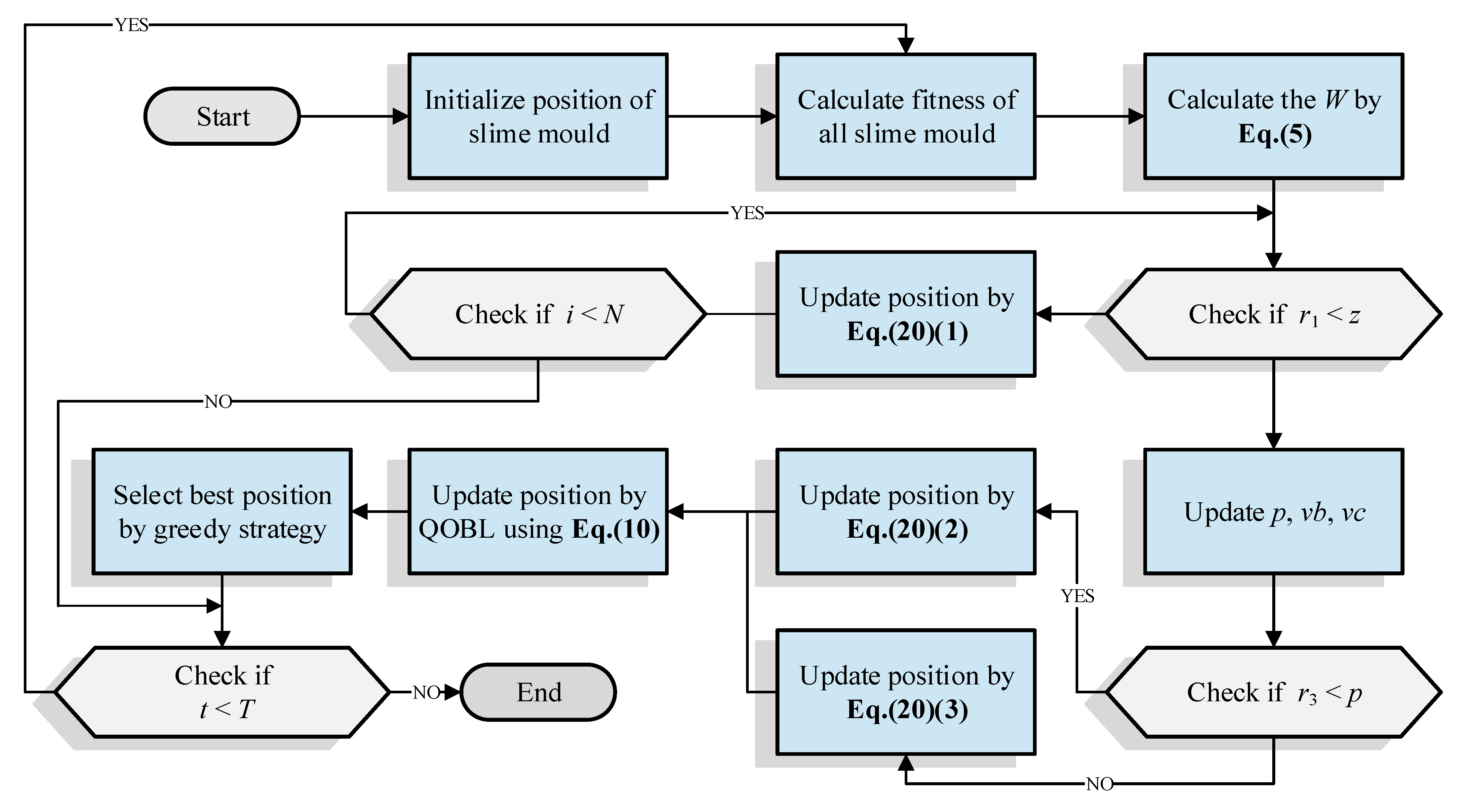
Secondly, quasi opposition-based learning was used to enhance the exploitation ability of SMA and balance the exploration and exploitation capability. The pseudo-code of ESMA is shown in Algorithm 2, and Figure 3 illustrates the flowchart of the proposed algorithm.
| Algorithm 2 Pseudo-code of ESMA |
| Initialize the positions of search agent; |
| While current iteration < maximum iteration do |
| Check if any search agent goes beyond the search space and amend it; |
| Calculate the fitness of all slime mould; |
| For each search agent, do |
| Update positions by Equation (20); |
| End For |
| Apply QOBL strategy by Equation (10); |
| Select the best position into next iteration by greedy strategy; |
| t = t + 1; |
| End While |
| Return the best solution; |
3.2. Computational Complexity Analysis
As can be seen, the ESMA mainly contains three components: Initialization phase, fitness evaluation, and position update procedure. In the initialization phase, the complexity can be expressed as O(N×D), where N represents the population size, and D denotes the dimension size of problems. Besides, the proposed algorithm evaluates the fitness of all slime mould with the complexity of O(N). The position update phase in the ESMA requires O(N×D). During the position updating phase, we utilize the QOBL to improve the exploitation ability and balance the exploration and exploitation; thus the QOBL strategy requires O(N×D). In summary, the total computation complexity of ESMA can be expressed as O(N×D×T) for T iterations. So, it can be concluded that both the SMA and ESMA have the same computational complexity wise.
4. Experimental Results and Discussion
4.1. Definition of 23 Benchmark Functions
To evaluate the exploration ability, exploitation ability, and escaping from the local optima ability of ESMA, twenty-three benchmark functions, including unimodal (F1–F7), multimodal (F8–F13), and fixed-dimension multimodal (F14–F23), are introduced [52]. The description of these functions is shown in Table 1, Table 2 and Table 3. As can be seen, the unimodal benchmark functions have only one global optimal value, which is suitable for evaluating the algorithms’ exploitation capability. Unlike unimodal functions, the multimodal and fixed-dimension benchmark functions have multiple local optimal values and only one optimal global value; it is suitable for evaluating the exploration ability and escaping from local minima.
To verify the performance of the proposed ESMA, we compared it with seven other algorithms including slime mould algorithm (SMA) [35], remora optimization algorithm (ROA) [36], arithmetic optimization algorithm (AOA) [32], aquila optimizer (AO) [33], salp swarm algorithm (SSA) [30], whale optimization algorithm (WOA) [29], and sine cosine algorithm (SCA) [31]. These classical and state-of-the-art algorithms are proved to equip with excellent performance on some optimization problems. The details of these algorithms are listed as follows:
- SMA [35] was proposed by Li et al. in 2020 and simulates the behavior and morphological process of slime mould during foraging.
- ROA [36] was proposed by Jia et al. in 2021 and simulates the parasitic behavior of remora.
- AOA [32] was proposed by Abualigah et al. in 2021 and is inspired by the arithmetic operator in mathematics.
- AO [33] was proposed by Abualigah et al. in 2021 and is inspired by the Aquila’s behaviors in nature during the process of catching the prey.
- SSA [30] was proposed by Mirjalili et al. in 2017 and is inspired by the swarming behavior of salps when navigating and foraging in oceans.
- WOA [29] was proposed by Mirjalili et al. in 2016 and mimics the social behavior of humpback whales.
- SCA [31] was proposed by Mirjalili et al. in 2016 and is inspired by the sine function and cosine function in nature.
Table 4 illustrates the parameter setting of each algorithm. For all the algorithms included in the comparison, we set the population size N = 30, dimension size D = 30, and maximum iteration T = 500; all the tests had 30 independent runs. Furthermore, we extract the average results, standard deviations, and statistical tests to evaluate the performance; the best results will be listed in bold font.
4.2. Statistical Results on 23 Benchmark Functions
The statistical results on 23 benchmark functions can be seen in Table 5. From this table, it can be clearly seen that the ESMA is superior to other algorithms in most benchmark functions. For unimodal benchmark functions (F1–F7), ESMA can obtain theoretical optimal for F1 and F3, while others algorithms cannot find the optimal solution. While ESMA cannot find the theoretical optimal for F4, F5, and F7, the convergence accuracy and robustness are better than other algorithms. In general, the exploitation ability of SMA is enhanced by applying the QOBL strategy. For the multimodal benchmark functions and fixed-dimension multimodal benchmark functions, ESMA also provides more competitive results than others. ESMA can obtain the theoretical optimal for F8, F9, F11, F14, F16, F17, F19, and F21–F23. For F10, F12, F13, and F15, ESMA gets the optimal global solution compared to others. Consequently, it can be concluded that ESMA always maintains high convergence accuracy and high robustness compared to other algorithms on such benchmark functions.
4.3. Wilcoxon Rank-Sum Test
In order to verify the non-incidentalness of the experimental results, this paper carried out the Wilcoxon rank-sum test (WRS). WRS is a nonparametric statistical test used to test the statistical performance between the proposed algorithm and comparison group on different benchmark functions [53]. WRS is based here on a 5% significant level, if the p-values obtained are less than 0.05, it indicates that there is a significant difference between them; otherwise, the difference is not obvious. The p-values obtained by algorithms are listed in Table 6. From this table, we can see that ESMA provides the statistically significant results compared with other algorithms.
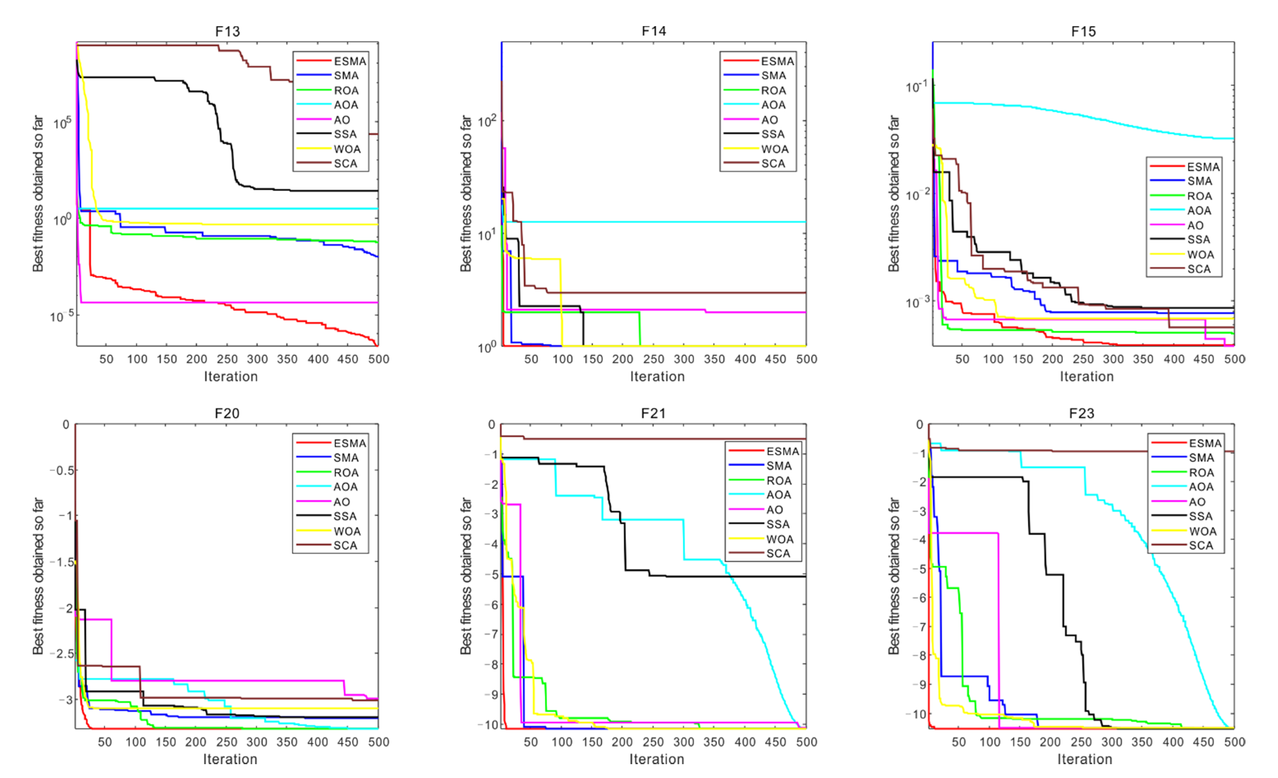
4.4. Convergence Behavior Analysis
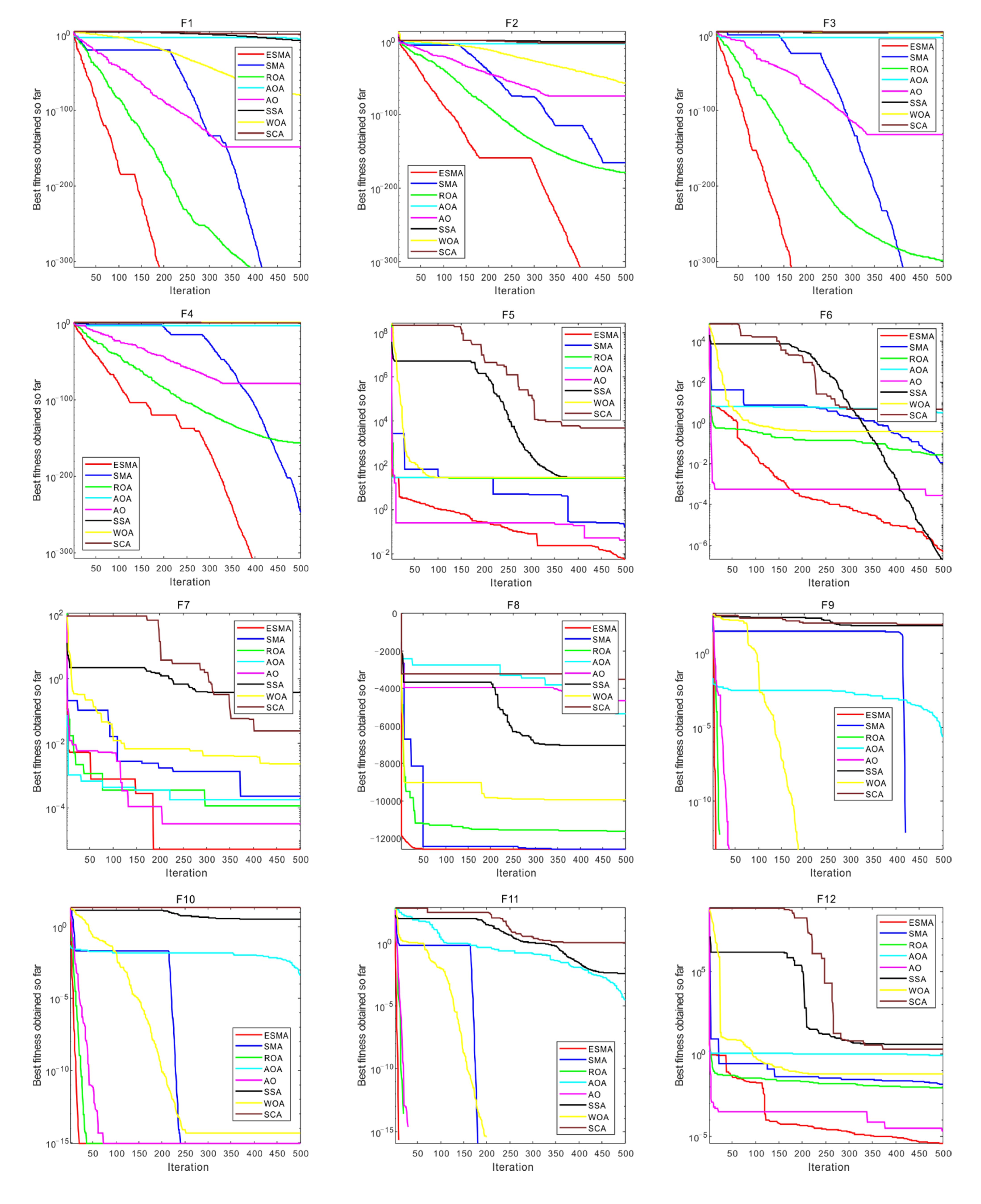
The convergence behavior of some benchmark functions is shown in Figure 4. On the unimodal benchmark functions, ESMA can achieve the highest accuracy and faster convergence speed. Especially for F1 and F3, while SMA can find the optimal solution, the convergence speed is slower than ESMA. For F2 and F4, ESMA finally converges to the optimal solution, while other algorithms either converge slowly or cannot converge to the optimal solution. For F5 and F7, while ESMA does not find the theoretical optimal solution, it still converges to the global optimal solution. On the multimodal benchmark functions, ESMA still shows the fastest convergence speed on most functions. While the global optimal solution is not found in some functions, it still has good performance compared with other algorithms. On the fixed dimensional multimodal functions, ESMA shows a faster convergence speed in the initial stage than others, and it also has a good convergence speed.
Generally, ESMA can obtain competitive results compared to other algorithms, such as the fastest convergence speed and highest convergence accuracy.
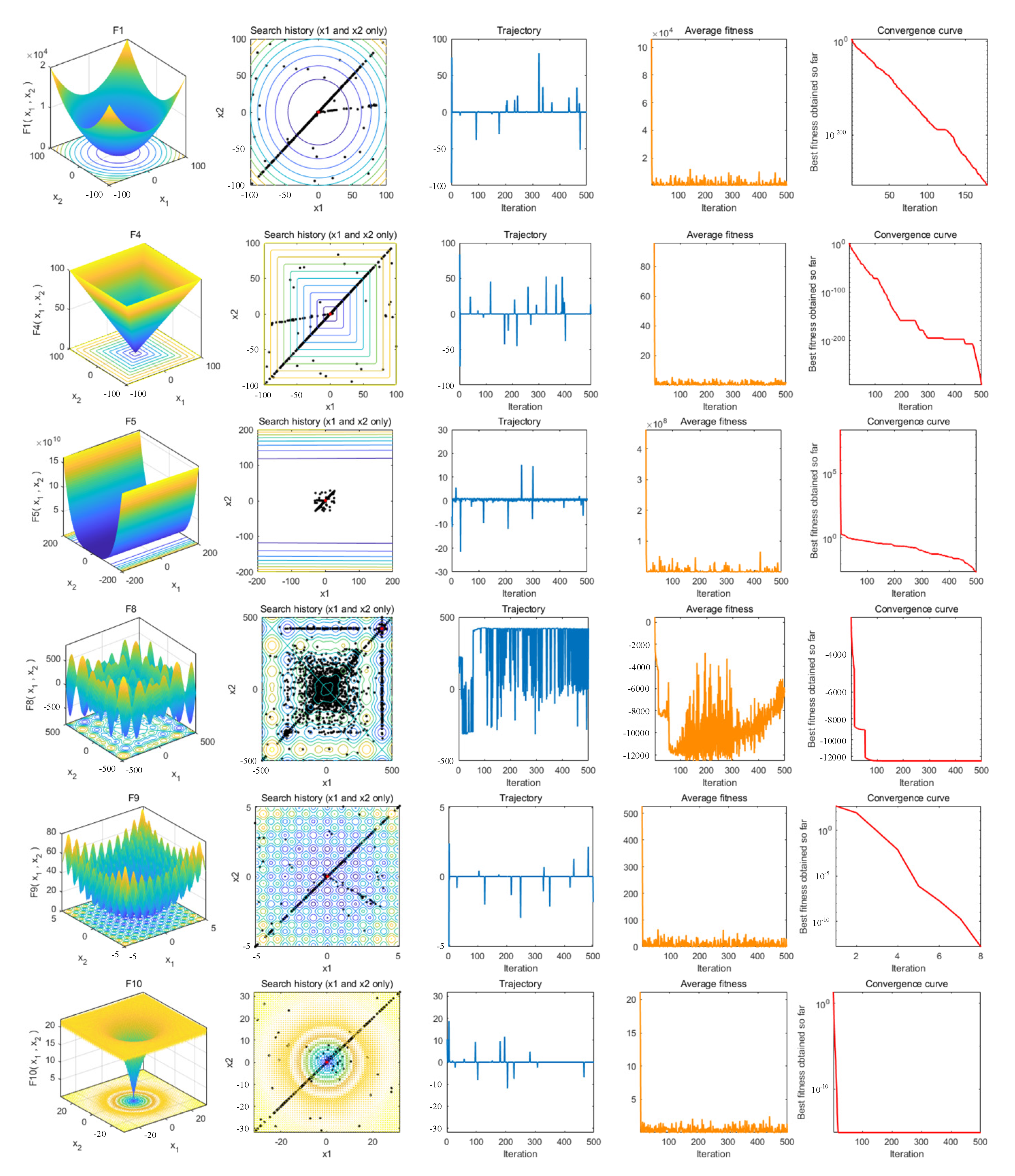
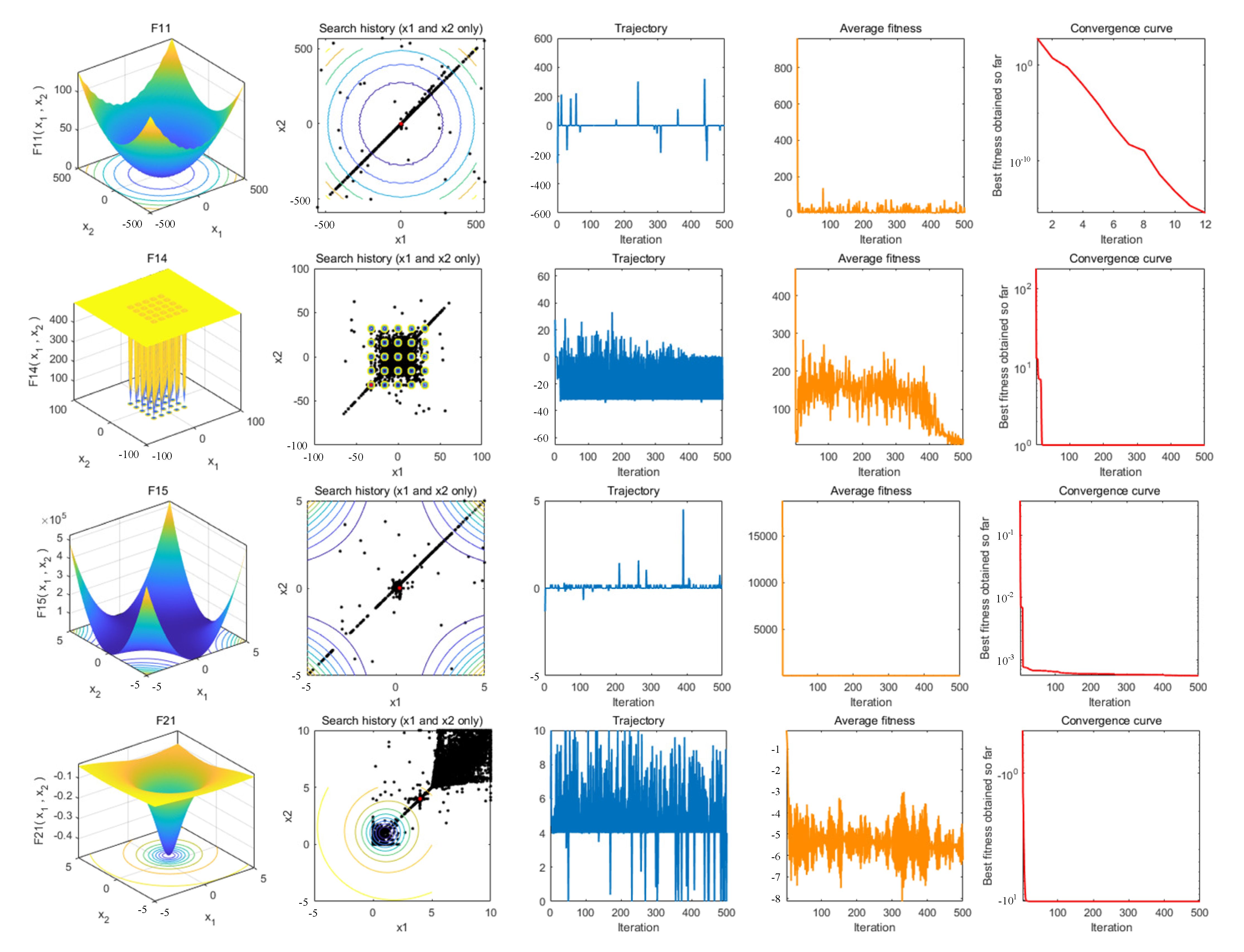
4.5. Qualitative Metrics Analysis
To evaluate the optimization performance of ESMA, Figure 5 illustrates the qualitative metrics, which include the 2D shape of benchmark functions (first column), search history of individuals (second column), trajectory (third column), average fitness (fourth column), and convergence curve (fifth column). For the first column, the 2D view of benchmark functions is described and shows the complexity of different functions. The second column illustrates the search history of the search agent from the first to the last iteration; it can be seen that the proposed ESMA is able to find the areas where the fitness values are the lowest. The trajectory of the first agent in the first dimension is described in the third column. We can see that the search agent oscillates continuously in the search space, which shows that the search agent widely studies the most promising fields and better solutions. The fourth column denotes the average fitness history. It can be seen that the fitness curve is decreasing, which indicates that the quality of the population is improving at each iteration. The last column is the convergence curve, which reveals that populations find the best solution after each iteration.
5. Experimental Results on Multilevel Thresholding
This section introduces the experimental details of the proposed algorithm ESMA applied to the multilevel thresholding image segmentation. First, the benchmark images and the experimental setup are presented in Section 5.1. Furthermore, the results of the algorithms in fitness, PSNR, SSIM, and FSIM are also analyzed. This section also shows the statistical analysis used to compare the proposed algorithm with other competitive algorithms.
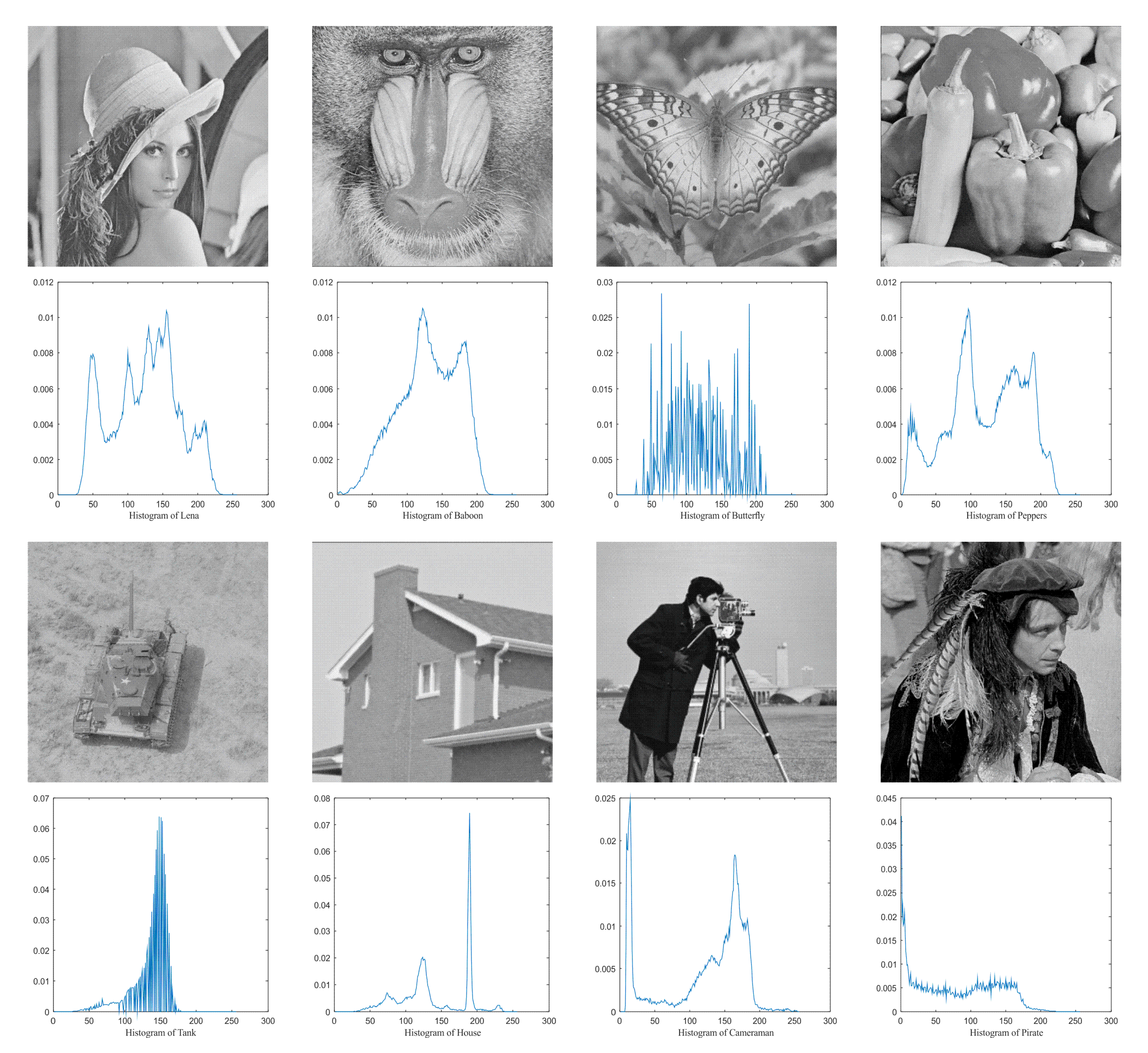
5.1. Experiment Setup
In this paper, the benchmark greyscale images, including Lena, Baboon, Butterfly, etc., are used to evaluate the performance of the proposed algorithm ESMA’s image segmentation [54]. All the benchmark images and their histogram images are represented in Figure 6. To guarantee the fairness of the experiment, all the algorithms are evaluated 30 times per image, and the maximum iteration T is 500; the number of population size N is 30. The number of thresholds values [nTh = 4, 6, 8, 10].
5.2. Evaluation Measurements
In this paper, three common evaluation methods are used to illustrate the performance of the algorithm and the quality of image segmentation, namely PSNR, FSIM, and SSIM, which are defined as follows:
5.2.1. PSNR
Peak Signal to Noise Ratio (PSNR) is an image quality evaluation metric used to evaluate the similarity between the original image and the segmented image [55]. The PSNR is calculated as:
where I and Seg denote the original image and segmented image with M × N, respectively; RMSE is the root mean square error.
5.2.2. SSIM
Structural Similarity (SSIM) is a common metric used to measure the structural similarity between the original image and the segmented image [3], and is defined as:
where μI and μSeg indicate the mean intensity of the original image and its segmented image; σI and σSeg denote the standard deviation of the original image and its segmented image; σI,Seg is the covariance of the original image and the segmented image. c1 and c2 are constant.
5.2.3. FSIM
Feature Similarity (FSIM) is used to estimate the structural similarity between the original image and the segmented image [56], and is defined as:
where Ω indicates the entire image domain; PC1 and PC2 represent the phase consistency of the original image and its segmented image, respectively; G1 and G2 represent the gradient magnitude of the original image and segmented image, respectively. T1 and T2 both are constant.
5.3. Experimental Result Analysis
This section mainly compares ESMA with seven optimization algorithms: SMA, ROA, AOA, AO, SSA, WOA, and SCA. All the algorithms run independently 30 times, and the average value (mean) and standard deviation (Std) are selected as the evaluation indexes, in which the best values are marked in bold.
Table A1 illustrates the optimal threshold values obtained by different algorithms on the benchmark images. It can be seen that when the number of thresholds is equal to 4 and 6, the thresholds obtained by most algorithms are roughly the same. However, the results are quite different when the thresholds are extended to 8 and 10, especially for SCA and AOA.
Table A2 represents the average fitness values and their Std obtained by all algorithms on the benchmark images. In general, the lower value of the average fitness denotes the better quality of segmentation. It can be seen that the fitness value of ESMA is better than most algorithms. For example, when the tank image is segmented with ten threshold levels, the fitness value obtained by ESMA ranks first, which is greatly improved compared with the SMA. Experimental results show that ESMA has better performance and strong applicability in segmenting multilevel threshold images.
Table A3 shows the PSNR results obtained by all algorithms. As mentioned above, it is suitable to evaluate the similarity between the segmented image and the original image, where a higher average value indicates a better segmentation quality. From the attained results, however, there are only small differences between the ESMA and other compared algorithms in threshold values 4 and 6. However, the PSNR values significantly increase when the threshold values are increasing. It can be observed that, for most benchmark images, the proposed ESMA significantly produces more favorable and reliable results than the original SMA and other compared algorithms, which provides better PSNR results for most benchmark images, for example, when images Lena, Baboon, Tank, Cameraman, and Pirate are tackled with 10 threshold levels. Obviously, the PSNR values are highest, and AO and WOA are ranked second and third, respectively. When segmenting Lena and Baboon images, ESMA showed the best PSNR value among all thresholds. Generally, ESMA presents the best performance with the images Lena, Baboon, Peppers, Tank, and House.
Table A4 illustrates the SSIM value obtained from different algorithms. As is possible to obverse, when the threshold is equal to 4, the SSIM results of each algorithm are roughly the same. Then, as the number of threshold values increases, the value of SSIM continues to increase, ESMA can obtain more original image information than other algorithms. For example, when the threshold value is equal to 4, the SSIM value obtained by ESMA for Baboon is 0.8041. When the number of thresholds increases to 10, the SSIM is 0.9395. Furthermore, when the threshold is equal to 6, 8, and 10, the segmentation quality of ESMA is better than most comparison algorithms, especially for segmenting Baboon, Butterfly, and House. In the case of Cameraman, the best SSIM results were obtained by ROA in the threshold values 4, 6, and 8. Overall, ESMA ranked first in segmentation quality.
Table A5 shows the FSIM values obtained by different algorithms, where a higher value represents the best quality of the segmentation. We can see that the SMA and ROA show significant performance in Baboon, Butterfly, and Cameraman. Both AOA and SCA are not shown a significant performance for any of the images. The proposed ESMA can achieve good results in segmenting most images. For example, when the House image is processed using eight each threshold level, the value of FSIM is significant. Therefore, in most cases, the algorithm proposed in this paper can extract the interesting target from the image more accurately.
Table A6 represents the p-value obtained by Wilcoxon rank-sum test with 5% significance level. It can be seen from the results that ESMA is significantly different from ROA, AOA, SSA, and SCA, which means that the proposed algorithm ESMA has been improved considerably. However, there is no significant difference at Lena for level 4. When comparing ESMA and WOA, there are significant differences in other images except for Butterfly, House, and Pepper.
Table 7 shows the image segmentation results of the proposed algorithm ESMA for different thresholds, in which the obtained optimal threshold is marked with a red vertical line. This table shows how the thresholds divide an image into several different classes and how the objects are segmented from the background.
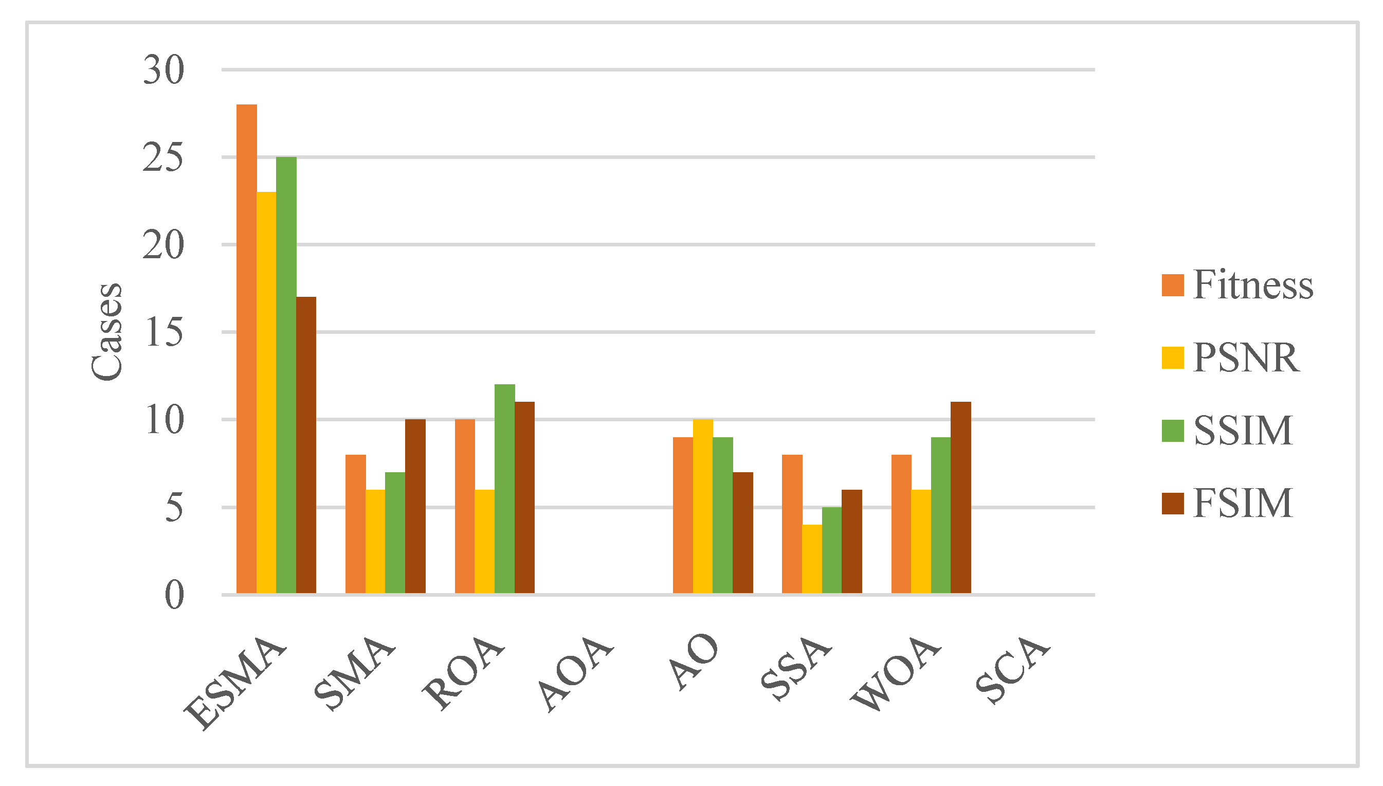
Figure 7 summarizes the segmentation experimental results of fitness, PSNR, SSIM, and FSIM based on the objective function. From this figure, we can see that the segmentation performance of ESMA is significantly improved compared with original SMA, and ROA and WOA are ranked second and third, respectively.
According to the above evaluation metrics and statistical test, the proposed ESMA has a better segmentation quality than other compared algorithms. Thus, the proposed ESMA can be effectively applied to the field of image segmentation.
6. Conclusions and Future Work
In this paper, an enhanced slime mould algorithm (ESMA) is proposed for global optimization and multilevel thresholding image segmentation. In order to improve the performance of SMA, we use two strategies. First, the Levy flight strategy is used to enhance the exploration ability. Second, quasi opposition-based learning is used to enhance the exploitation ability and balance the exploration and exploitation. To evaluate the performance of ESMA, ESMA and some state-of-the-art algorithms were tested on the 23 benchmark functions, and the results indicate that the ESMA is superior to others. This shows that the above two strategies can effectively help SMA avoid falling into optimal local state and improve the global search ability of the population. In addition, we applied ESMA to multilevel thresholding image segmentation, and minimum cross-entropy is selected as the fitness function. The experimental evaluation metrics determined the mean fitness, standard deviation, PSNR, SSIM, FSIM and Wilcoxon rank-sum test. Experimental results show that the ESMA method is superior to other image segmentation methods in PSNR, FSIM, SSIM, and statistical tests.
While the proposed work is valuable in the image segmentation field, it is necessary to extend the benchmark images and increase the number of thresholds to obtain more reliable results. In addition, we will also seek to hybridize the ESMA with other MAs to improve the segmentation results when solving real-world applications, such as ship target segmentation and medical image segmentation. Meanwhile, other objective functions can be selected to realize multilevel thresholding image segmentation.
Author Contributions
S.L., methodology, software, validation, formal analysis, investigation, resources, writing—original draft preparation, funding acquisition; H.J., conceptualization, writing—review and editing, visualization, supervision; L.A., review and editing, supervision; M.A., review and editing. All authors have read and agreed to the published version of the manuscript.
Funding
This research is funded by the High-tech Ship Research Program (No. [2017]614 and No. [2018]473) from Ministry of Industry and Information Technology of China, Fujian Natural Science Foundation Project (2021J011128), Sanming University National Natural Science Foundation Breeding Project (PYT2105), Sanming University Introduces High-level Talents to Start Scientific Research Funding Support Project (20YG14). This study was financially supported via a funding grant by Deanship of Scientific Research, Taif University Researchers Supporting Project number (TURSP-2020/300), Taif University, Taif, Saudi Arabia.
Institutional Review Board Statement
Not applicable.
Informed Consent Statement
Not applicable.
Data Availability Statement
The data presented in this study are available on request from the corresponding author.
Conflicts of Interest
The author declares no conflict of interest.
Appendix A

Table A1.
The best thresholds obtained by algorithms.
| Image | nTh | ESMA | SMA | ROA | AOA | AO | SSA | WOA | SCA |
|---|---|---|---|---|---|---|---|---|---|
| Lena | 4 | 71 109 141 177 | 71 109 141 177 | 71 109 141 177 | 78 112 147 200 | 71 109 141 177 | 71 109 141 177 | 71 109 141 177 | 78 105 142 181 |
| 6 | 60 86 113 137 160 187 | 60 85 112 137 160 187 | 60 86 113 137 160 187 | 17 47 53 91 134 176 | 60 86 113 137 160 187 | 60 86 113 137 160 187 | 60 86 113 137 160 187 | 58 87 105 136 153 186 | |
| 8 | 52 69 90 111 130 147 166 191 | 50 65 84 102 121 142 163 189 | 2 52 70 93 116 139 161 188 | 62 87 109 122 142 164 182 189 | 52 69 90 111 130 147 166 191 | 52 69 90 111 130 147 166 191 | 52 69 90 111 130 147 166 191 | 1 53 76 101 121 137 165 189 | |
| 10 | 48 60 75 91 107 122 137 152 169 193 | 50 65 83 100 117 134 149 165 184 203 | 47 59 73 90 106 121 137 152 169 193 | 17 45 55 68 78 110 141 155 170 201 | 3 50 64 82 99 116 134 151 169 193 | 49 62 78 95 110 126 141 155 172 194 | 2 50 65 83 100 117 135 151 169 193 | 1 47 50 71 77 92 110 138 164 187 | |
| Baboon | 4 | 65 100 132 164 | 64 99 131 164 | 65 100 132 164 | 47 92 141 190 | 65 100 132 164 | 65 100 132 164 | 65 100 132 164 | 61 98 134 169 |
| 6 | 49 75 100 123 146 172 | 47 73 98 121 145 172 | 49 75 100 123 146 172 | 46 69 102 142 179 179 | 49 75 100 123 146 172 | 49 75 100 123 146 172 | 49 75 100 123 146 172 | 38 56 83 114 135 158 | |
| 8 | 40 63 83 103 122 140 160 180 | 34 55 74 94 114 133 154 177 | 39 61 81 101 119 137 158 179 | 70 94 118 154 157 184 190 194 | 38 61 81 101 119 137 158 179 | 39 62 82 102 121 139 159 180 | 39 61 81 101 119 137 158 179 | 1 1 26 59 88 113 137 175 | |
| 10 | 32 52 69 86 102 117 132 149 167 185 | 25 46 62 79 96 113 129 146 164 182 | 9 40 59 77 95 112 128 145 164 183 | 28 41 64 89 114 125 156 180 200 229 | 35 56 74 92 110 127 144 163 182 253 | 35 56 74 92 110 127 144 163 182 244 | 8 40 59 77 95 112 128 145 164 183 | 1 2 2 43 72 91 116 130 146 170 | |
| Butterfly | 4 | 70 97 125 161 | 70 97 125 161 | 70 97 125 161 | 69 108 147 226 | 70 97 125 161 | 70 97 125 161 | 70 97 125 161 | 64 90 119 163 |
| 6 | 61 83 103 127 153 180 | 61 83 103 127 153 181 | 61 83 103 127 153 180 | 42 66 75 96 135 154 | 61 82 103 127 153 180 | 61 82 103 127 153 180 | 61 82 103 127 153 181 | 1 62 85 111 136 169 | |
| 8 | 54 69 82 98 115 136 158 181 | 54 69 82 98 115 136 157 181 | 54 69 82 98 115 136 158 181 | 27 52 80 115 130 151 161 233 | 54 69 82 98 115 135 158 181 | 54 69 84 100 115 135 157 180 | 50 69 83 99 115 135 158 181 | 1 47 74 96 114 138 164 183 | |
| 10 | 26 54 69 83 96 111 127 143 160 182 | 31 50 68 83 96 111 127 142 160 182 | 26 54 69 83 96 111 127 143 160 182 | 35 44 56 57 66 91 104 136 158 202 | 2 44 57 70 84 100 115 135 158 180 | 12 54 69 83 96 111 127 142 160 182 | 33 54 66 82 97 112 127 142 161 182 | 1 55 61 68 88 105 112 128 149 174 | |
| Peppers | 4 | 37 76 118 164 | 37 77 119 165 | 37 77 119 165 | 53 61 109 142 | 37 77 119 165 | 37 77 119 165 | 37 77 119 165 | 35 72 118 168 |
| 6 | 25 49 78 108 140 174 | 32 62 88 115 146 177 | 25 49 78 108 140 174 | 13 41 59 102 152 176 | 24 48 78 108 140 174 | 25 49 78 108 140 174 | 25 49 78 108 140 174 | 1 36 78 114 141 169 | |
| 8 | 22 43 68 89 109 133 158 183 | 22 42 67 88 108 133 158 183 | 22 42 67 88 108 133 158 183 | 30 45 61 73 85 130 172 217 | 13 45 78 91 124 151 166 202 | 23 44 71 93 118 148 178 235 | 22 43 68 89 109 134 158 183 | 6 37 58 84 101 129 157 180 | |
| 10 | 20 36 55 74 91 109 131 153 174 196 | 16 26 41 59 77 94 113 137 160 184 | 11 26 45 62 87 97 122 141 174 199 | 2 17 30 71 83 98 125 147 152 205 | 17 43 72 80 102 126 148 157 167 204 | 22 42 67 87 106 128 151 173 195 236 | 2 22 42 67 87 106 128 151 173 195 | 1 1 20 31 55 83 110 136 168 250 | |
| Tank | 4 | 67 96 124 145 | 67 96 123 145 | 67 96 123 145 | 57 112 132 147 | 67 96 124 146 | 68 98 126 147 | 67 96 124 146 | 71 103 126 146 |
| 6 | 56 77 99 119 136 151 | 1 64 91 115 135 151 | 56 77 98 119 136 151 | 78 92 128 146 175 213 | 56 77 98 118 135 150 | 56 77 99 119 136 149 | 55 77 99 118 136 151 | 14 63 91 115 131 147 | |
| 8 | 55 74 93 109 123 138 147 156 | 52 71 90 106 122 135 147 156 | 2 55 76 95 114 128 141 152 | 50 89 119 126 150 196 200 241 | 1 3 56 77 99 118 136 149 | 55 76 95 114 129 142 152 251 | 54 75 93 111 127 139 149 159 | 1 1 51 72 94 119 128 149 | |
| 10 | 47 63 78 92 106 119 130 142 151 159 | 1 3 52 71 87 103 118 133 145 157 | 28 55 72 88 102 116 129 140 150 159 | 15 26 48 67 78 108 137 143 162 224 | 6 31 57 78 98 119 136 151 212 217 | 55 76 95 113 129 141 153 211 220 255 | 43 55 73 88 100 116 129 139 151 158 | 1 18 35 51 67 93 106 123 146 155 | |
| House | 4 | 63 90 115 157 | 63 90 115 157 | 63 90 115 157 | 63 104 161 217 | 63 90 115 157 | 63 90 115 157 | 63 90 115 157 | 60 85 116 154 |
| 6 | 61 85 106 122 141 173 | 63 89 113 138 170 207 | 63 89 113 138 170 207 | 33 66 88 114 137 156 | 63 89 113 138 170 207 | 63 89 113 138 170 207 | 63 89 113 138 170 207 | 2 68 97 115 156 218 | |
| 8 | 55 72 90 109 124 142 172 207 | 57 75 92 110 124 142 172 207 | 55 72 90 109 124 142 172 207 | 6 38 76 97 141 162 180 214 | 55 73 91 110 124 142 172 207 | 12 59 78 96 116 138 170 207 | 55 72 90 109 124 142 172 207 | 1 1 65 95 118 135 162 207 | |
| 10 | 51 67 80 94 109 121 130 146 173 207 | 2 51 66 80 95 111 125 143 172 207 | 6 51 67 81 96 112 125 143 172 207 | 57 76 94 102 124 144 165 169 182 221 | 32 51 67 81 95 112 125 143 172 207 | 13 55 72 90 109 124 142 172 207 244 | 55 72 90 110 124 142 171 189 199 218 | 1 58 80 90 109 131 150 184 205 224 | |
| Cameraman | 4 | 29 76 125 158 | 29 76 125 158 | 29 76 125 158 | 16 40 91 140 | 29 76 125 158 | 29 76 125 158 | 29 76 125 158 | 27 78 135 167 |
| 6 | 23 49 85 121 148 173 | 23 49 85 121 148 173 | 23 49 85 121 148 173 | 7 21 43 78 116 153 | 23 49 85 121 148 173 | 23 49 85 121 148 173 | 23 48 85 120 148 173 | 21 43 93 124 149 175 | |
| 8 | 23 47 80 112 135 155 173 202 | 15 26 50 83 115 138 158 177 | 23 47 80 112 135 155 173 202 | 23 52 105 112 129 148 161 172 | 23 47 80 112 134 155 173 202 | 15 26 50 82 114 137 157 177 | 23 48 81 112 135 155 173 202 | 1 1 20 45 86 124 147 171 | |
| 10 | 14 25 47 75 102 122 141 158 174 202 | 14 23 39 60 88 116 137 156 173 202 | 14 21 34 56 86 115 137 156 173 202 | 33 53 76 91 141 159 168 241 250 253 | 14 28 52 80 105 123 141 156 172 200 | 14 25 49 82 113 135 155 173 197 230 | 14 23 39 61 89 117 138 157 174 202 | 1 15 20 38 57 91 127 145 163 219 | |
| Pirate | 4 | 13 41 82 130 | 13 41 82 130 | 13 41 82 130 | 7 21 58 95 | 13 41 82 130 | 13 41 82 130 | 13 41 82 130 | 13 41 81 124 |
| 6 | 8 24 48 80 114 147 | 8 24 48 80 114 147 | 8 24 49 81 115 148 | 19 70 97 103 157 254 | 8 24 49 81 115 148 | 8 24 48 80 114 147 | 8 24 49 81 115 148 | 8 21 50 84 122 162 | |
| 8 | 5 14 29 48 71 97 125 153 | 5 14 30 49 72 98 125 153 | 5 13 27 46 68 94 123 152 | 12 35 54 68 94 142 157 164 | 5 14 29 48 71 97 125 153 | 5 15 33 55 83 113 140 170 | 7 20 41 66 96 126 154 223 | 4 12 15 24 47 82 114 148 | |
| 10 | 4 10 21 36 53 73 96 120 144 169 | 4 9 17 28 42 60 81 105 130 156 | 3 8 16 28 43 61 82 106 130 156 | 8 28 41 67 98 126 137 145 151 162 | 4 10 21 36 55 77 101 127 155 240 | 5 14 29 49 71 96 122 148 177 254 | 5 14 29 49 72 97 123 148 183 210 | 1 4 12 29 41 71 83 114 136 163 |
Table A2.
The fitness values obtained by algorithms.
| Image | nTh | ESMA | SMA | ROA | AOA | AO | SSA | WOA | SCA | ||||||||
|---|---|---|---|---|---|---|---|---|---|---|---|---|---|---|---|---|---|
| Mean | Std | Mean | Std | Mean | Std | Mean | Std | Mean | Std | Mean | Std | Mean | Std | Mean | Std | ||
| Lena | 4 | 0.4611 | 0 | 0.4611 | 0 | 0.4611 | 0 | 0.7091 | 0.1235 | 0.4611 | 0 | 0.4611 | 0 | 0.4774 | 0.0621 | 0.513 | 0.0796 |
| 6 | 0.245 | 0.0063 | 0.249 | 0.0142 | 0.2481 | 0.004 | 0.4945 | 0.0972 | 0.2567 | 0.0264 | 0.2473 | 0.0045 | 0.2481 | 0.014 | 0.3337 | 0.0464 | |
| 8 | 0.1512 | 0.0017 | 0.1634 | 0.0174 | 0.1569 | 0.0019 | 0.3348 | 0.063 | 0.1557 | 0.0127 | 0.1624 | 0.0169 | 0.1556 | 0.0127 | 0.243 | 0.0337 | |
| 10 | 0.1048 | 0.0015 | 0.1199 | 0.0169 | 0.1093 | 0.0087 | 0.2594 | 0.0366 | 0.1083 | 0.0081 | 0.113 | 0.01 | 0.1122 | 0.0119 | 0.1921 | 0.0238 | |
| Baboon | 4 | 0.4962 | 0 | 0.4962 | 0 | 0.4962 | 0 | 0.7593 | 0.1236 | 0.4962 | 0 | 0.4962 | 0 | 0.4962 | 0 | 0.5342 | 0.0598 |
| 6 | 0.2781 | 0.0001 | 0.2785 | 0.0003 | 0.2782 | 0 | 0.4957 | 0.0791 | 0.281 | 0.0151 | 0.2783 | 0.0001 | 0.2806 | 0.0131 | 0.3507 | 0.0404 | |
| 8 | 0.178 | 0.0004 | 0.1805 | 0.0054 | 0.1784 | 0.0037 | 0.3544 | 0.0477 | 0.1789 | 0.0073 | 0.1868 | 0.0165 | 0.1783 | 0.004 | 0.2683 | 0.0396 | |
| 10 | 0.1229 | 0.0004 | 0.1293 | 0.0075 | 0.123 | 0.0017 | 0.2625 | 0.0311 | 0.1248 | 0.0071 | 0.1387 | 0.0149 | 0.1256 | 0.0081 | 0.2136 | 0.0275 | |
| Butterfly | 4 | 0.3968 | 0 | 0.3968 | 0 | 0.3968 | 0 | 0.7151 | 0.1365 | 0.3968 | 0 | 0.3968 | 0 | 0.4116 | 0.0561 | 0.4669 | 0.0886 |
| 6 | 0.229 | 0.0043 | 0.2297 | 0.0184 | 0.2348 | 0.0278 | 0.4595 | 0.0859 | 0.229 | 0.0134 | 0.2292 | 0.0135 | 0.2372 | 0.0298 | 0.3061 | 0.0367 | |
| 8 | 0.1356 | 0.0141 | 0.1413 | 0.0181 | 0.1385 | 0.0224 | 0.305 | 0.0517 | 0.1389 | 0.007 | 0.1383 | 0.0157 | 0.138 | 0.0165 | 0.2219 | 0.0258 | |
| 10 | 0.0853 | 0.0039 | 0.1069 | 0.0157 | 0.0923 | 0.0097 | 0.244 | 0.0463 | 0.0926 | 0.0088 | 0.1059 | 0.0151 | 0.0969 | 0.015 | 0.1774 | 0.0244 | |
| Peppers | 4 | 0.704 | 0 | 0.704 | 0 | 0.704 | 0 | 1.0897 | 0.1784 | 0.704 | 0 | 0.704 | 0 | 0.704 | 0 | 0.7277 | 0.015 |
| 6 | 0.4019 | 0.0027 | 0.4007 | 0.0019 | 0.3997 | 0.0003 | 0.6925 | 0.0853 | 0.3998 | 0.0003 | 0.4002 | 0.0013 | 0.3997 | 0.0001 | 0.4913 | 0.0585 | |
| 8 | 0.2456 | 0.0001 | 0.2481 | 0.0059 | 0.246 | 0.0025 | 0.4845 | 0.067 | 0.2459 | 0.0001 | 0.256 | 0.0237 | 0.2459 | 0.0001 | 0.3663 | 0.0361 | |
| 10 | 0.1755 | 0.0057 | 0.1779 | 0.0128 | 0.1793 | 0.0003 | 0.3631 | 0.0607 | 0.1792 | 0.0001 | 0.1931 | 0.0196 | 0.1792 | 0.0002 | 0.2913 | 0.0317 | |
| Tank | 4 | 0.1992 | 0.0001 | 0.1993 | 0.0001 | 0.1992 | 0 | 0.3468 | 0.0542 | 0.1992 | 0 | 0.1992 | 0.0001 | 0.2026 | 0.0182 | 0.2184 | 0.0292 |
| 6 | 0.106 | 0.0012 | 0.1153 | 0.015 | 0.1069 | 0.0002 | 0.2579 | 0.0519 | 0.1127 | 0.0136 | 0.1171 | 0.0161 | 0.1106 | 0.0114 | 0.1694 | 0.0246 | |
| 8 | 0.0707 | 0.0022 | 0.0816 | 0.0148 | 0.0797 | 0.0078 | 0.1962 | 0.0468 | 0.0709 | 0.0058 | 0.0774 | 0.0089 | 0.0726 | 0.0092 | 0.1395 | 0.0196 | |
| 10 | 0.045 | 0.0048 | 0.0655 | 0.0126 | 0.049 | 0.006 | 0.1462 | 0.029 | 0.0524 | 0.0072 | 0.0612 | 0.0098 | 0.0521 | 0.0063 | 0.1024 | 0.0173 | |
| House | 4 | 0.3302 | 0.0093 | 0.3302 | 0 | 0.3345 | 0.0237 | 0.478 | 0.0713 | 0.3302 | 0 | 0.3302 | 0 | 0.3302 | 0.0001 | 0.3512 | 0.0313 |
| 6 | 0.1816 | 0.0245 | 0.1606 | 0 | 0.1658 | 0.0197 | 0.3072 | 0.0429 | 0.1634 | 0.0153 | 0.1632 | 0.0142 | 0.1632 | 0.0142 | 0.2239 | 0.0329 | |
| 8 | 0.0964 | 0.0127 | 0.1018 | 0.0131 | 0.1009 | 0.0155 | 0.2271 | 0.034 | 0.0966 | 0.0078 | 0.1031 | 0.0128 | 0.1025 | 0.0134 | 0.1552 | 0.0198 | |
| 10 | 0.0665 | 0.0019 | 0.0773 | 0.0112 | 0.0669 | 0.0028 | 0.1686 | 0.0292 | 0.0705 | 0.0065 | 0.0715 | 0.0053 | 0.0714 | 0.0057 | 0.1246 | 0.0194 | |
| Cameraman | 4 | 0.5385 | 0 | 0.5385 | 0 | 0.5385 | 0 | 0.7752 | 0.1214 | 0.5385 | 0 | 0.5385 | 0 | 0.5385 | 0 | 0.5506 | 0.0067 |
| 6 | 0.3032 | 0 | 0.3033 | 0 | 0.3033 | 0.0001 | 0.5071 | 0.076 | 0.3033 | 0 | 0.3105 | 0.0166 | 0.3033 | 0.0002 | 0.3682 | 0.0478 | |
| 8 | 0.2031 | 0.0042 | 0.2061 | 0.0063 | 0.2077 | 0.0117 | 0.3548 | 0.0569 | 0.2041 | 0.0021 | 0.2046 | 0.0015 | 0.2049 | 0.0087 | 0.2823 | 0.0431 | |
| 10 | 0.1368 | 0.0103 | 0.1396 | 0.0152 | 0.139 | 0.0088 | 0.2832 | 0.0426 | 0.1387 | 0.0061 | 0.1427 | 0.013 | 0.1383 | 0.0054 | 0.2299 | 0.0209 | |
| Pirate | 4 | 1.0403 | 0 | 1.0403 | 0 | 1.0403 | 0 | 1.6838 | 0.3576 | 1.0403 | 0 | 1.0403 | 0 | 1.0403 | 0 | 1.0588 | 0.0117 |
| 6 | 0.5845 | 0.0045 | 0.5822 | 0.0016 | 0.5815 | 0 | 1.1018 | 0.2407 | 0.5815 | 0 | 0.5937 | 0.0458 | 0.5815 | 0.0001 | 0.6456 | 0.0341 | |
| 8 | 0.3593 | 0.0023 | 0.3599 | 0.0026 | 0.3576 | 0.0002 | 0.8182 | 0.1572 | 0.3577 | 0.0004 | 0.3904 | 0.0317 | 0.3576 | 0.0002 | 0.4814 | 0.0636 | |
| 10 | 0.2413 | 0.0058 | 0.2499 | 0.0056 | 0.2445 | 0.0007 | 0.6187 | 0.1055 | 0.2461 | 0.0095 | 0.3038 | 0.023 | 0.2443 | 0.0006 | 0.3821 | 0.0403 | |
Table A3.
The PSNR values obtained by algorithms.
| Image | nTh | ESMA | SMA | ROA | AOA | AO | SSA | WOA | SCA | ||||||||
|---|---|---|---|---|---|---|---|---|---|---|---|---|---|---|---|---|---|
| Mean | Std | Mean | Std | Mean | Std | Mean | Std | Mean | Std | Mean | Std | Mean | Std | Mean | Std | ||
| Lena | 4 | 18.7867 | 0 | 18.7867 | 0 | 18.7867 | 0 | 17.9115 | 0.7829 | 18.7867 | 0 | 18.7867 | 0 | 18.7211 | 0.257 | 18.5889 | 0.4204 |
| 6 | 21.1436 | 0.3611 | 20.9155 | 0.201 | 20.9023 | 0.0791 | 19.6602 | 1.0424 | 20.9171 | 0.2101 | 20.9881 | 0.2528 | 20.888 | 0.0102 | 20.7039 | 0.8201 | |
| 8 | 23.3637 | 0.1453 | 23.2477 | 0.5122 | 23.3548 | 0.1958 | 21.3528 | 1.3934 | 23.2899 | 0.2038 | 23.3507 | 0.5784 | 23.3314 | 0.3472 | 22.7486 | 1.2342 | |
| 10 | 25.3269 | 0.329 | 24.9085 | 0.8677 | 25.255 | 0.5987 | 22.5184 | 1.6544 | 25.0865 | 0.5052 | 24.667 | 0.4771 | 25.3044 | 0.6412 | 23.8616 | 1.4136 | |
| Baboon | 4 | 20.7335 | 0.0247 | 20.7335 | 0.0247 | 20.7215 | 0.0157 | 18.8128 | 1.0221 | 20.7215 | 0.0157 | 20.7163 | 0 | 20.7198 | 0.0131 | 20.4913 | 0.5255 |
| 6 | 24.195 | 0.0307 | 24.1869 | 0.0354 | 24.1523 | 0 | 21.2006 | 0.9268 | 24.1063 | 0.2569 | 24.1673 | 0.02 | 24.1101 | 0.2313 | 22.936 | 0.6118 | |
| 8 | 26.5418 | 0.0426 | 26.4394 | 0.2024 | 26.5412 | 0.1283 | 22.8569 | 0.9407 | 26.5353 | 0.1962 | 26.3104 | 0.4386 | 26.5417 | 0.1499 | 24.4069 | 0.707 | |
| 10 | 28.3939 | 0.07 | 27.9523 | 0.3452 | 28.3236 | 0.1161 | 24.3764 | 0.6605 | 28.2776 | 0.2594 | 27.7754 | 0.5268 | 28.2071 | 0.3548 | 25.566 | 0.6591 | |
| Butterfly | 4 | 19.384 | 0 | 19.384 | 0 | 19.384 | 0 | 17.3819 | 1.7028 | 19.384 | 0 | 19.3918 | 0.0237 | 19.3124 | 0.2727 | 18.8569 | 0.8241 |
| 6 | 23.027 | 0.3381 | 22.6981 | 0.3791 | 22.4712 | 0.1428 | 20.1249 | 1.5871 | 22.4572 | 0.1907 | 22.7495 | 0.4085 | 22.4194 | 0.3011 | 21.7811 | 1.2288 | |
| 8 | 25.2782 | 0.4232 | 25.1357 | 0.5241 | 25.281 | 0.464 | 22.6981 | 1.1545 | 25.2233 | 0.2508 | 25.0719 | 0.5173 | 25.6065 | 0.5072 | 23.4691 | 0.959 | |
| 10 | 27.8053 | 0.9404 | 26.9718 | 1.0735 | 27.7339 | 0.9339 | 23.6315 | 1.6794 | 26.9143 | 1.088 | 26.6992 | 1.2001 | 27.8357 | 0.9296 | 24.9351 | 1.0205 | |
| Peppers | 4 | 20.3048 | 0 | 20.2961 | 0.0175 | 20.3048 | 0 | 18.4579 | 1.0843 | 20.3048 | 0 | 20.3033 | 0.0079 | 20.3048 | 0 | 20.1694 | 0.2803 |
| 6 | 23.1363 | 0.1851 | 23.0465 | 0.131 | 22.9841 | 0.0193 | 20.6058 | 0.9365 | 22.9847 | 0.0241 | 23.0143 | 0.097 | 22.9755 | 0.0182 | 22.1766 | 0.5925 | |
| 8 | 25.4398 | 0.0251 | 25.3289 | 0.2152 | 25.4282 | 0.0478 | 22.2705 | 0.9964 | 25.4386 | 0.0236 | 25.2324 | 0.4713 | 25.4277 | 0.0225 | 23.3841 | 0.5773 | |
| 10 | 26.7164 | 0.213 | 26.6864 | 0.3272 | 26.9926 | 0.0468 | 23.7216 | 1.1374 | 27.0096 | 0.0336 | 26.5867 | 0.4785 | 26.986 | 0.0382 | 24.3768 | 0.5042 | |
| Tank | 4 | 23.621 | 0.1847 | 23.5904 | 0.1884 | 23.6233 | 0.1601 | 21.0197 | 1.3991 | 23.631 | 0.1665 | 23.619 | 0.1653 | 23.5073 | 0.4685 | 23.1379 | 0.8407 |
| 6 | 27.1319 | 0.1967 | 26.5793 | 0.8502 | 27.1103 | 0.1303 | 22.6586 | 1.6433 | 26.734 | 0.7977 | 26.4843 | 0.9135 | 26.9133 | 0.5067 | 24.8651 | 0.8758 | |
| 8 | 29.1754 | 0.3681 | 28.6313 | 0.9286 | 28.6987 | 0.3745 | 24.7671 | 1.168 | 28.6371 | 0.375 | 28.55 | 0.6137 | 28.6097 | 0.4403 | 26.1582 | 1.0087 | |
| 10 | 31.0145 | 0.325 | 29.9936 | 0.8134 | 30.9248 | 0.7471 | 25.8087 | 1.3187 | 30.1609 | 0.6403 | 29.7464 | 1.014 | 30.8067 | 0.5992 | 28.0394 | 1.0181 | |
| House | 4 | 19.6568 | 0 | 19.6568 | 0 | 19.6148 | 0.2299 | 18.4479 | 1.8064 | 19.6568 | 0 | 19.6568 | 0 | 19.6602 | 0.0129 | 19.3939 | 0.6208 |
| 6 | 22.8143 | 0.1219 | 22.7241 | 0.0352 | 22.5672 | 0.5813 | 21.1436 | 1.3549 | 22.6941 | 0.0906 | 22.6359 | 0.4089 | 22.6515 | 0.4135 | 21.6748 | 1.216 | |
| 8 | 24.6994 | 0.0803 | 24.4874 | 0.4175 | 24.6165 | 0.3892 | 22.5041 | 1.6702 | 24.642 | 0.2449 | 24.4491 | 0.4135 | 24.6646 | 0.2606 | 24.1296 | 1.4269 | |
| 10 | 25.9749 | 0.1114 | 25.6998 | 0.3883 | 26.0617 | 0.1936 | 23.7466 | 1.467 | 26.0764 | 0.5714 | 25.8552 | 0.4539 | 26.0151 | 0.2245 | 24.7753 | 1.5695 | |
| Cameraman | 4 | 21.4059 | 0 | 21.4059 | 0 | 21.4059 | 0 | 19.2516 | 1.3089 | 21.4059 | 0 | 21.4059 | 0 | 21.4021 | 0.0142 | 21.1921 | 0.4044 |
| 6 | 23.905 | 0 | 23.9124 | 0.019 | 23.911 | 0.0177 | 21.3045 | 1.2432 | 23.9102 | 0.0178 | 23.8265 | 0.1787 | 23.9187 | 0.0413 | 22.9911 | 0.8038 | |
| 8 | 25.5199 | 0.4548 | 25.411 | 0.4505 | 25.5124 | 0.4735 | 23.1434 | 1.1121 | 25.5978 | 0.395 | 25.7295 | 0.315 | 25.6113 | 0.4191 | 24.1015 | 0.7116 | |
| 10 | 27.5098 | 0.3286 | 27.1335 | 0.5009 | 27.1949 | 0.439 | 24.3376 | 1.1574 | 27.487 | 0.3557 | 27.3671 | 0.4647 | 27.303 | 0.2443 | 24.9613 | 0.8164 | |
| Pirate | 4 | 20.9183 | 0 | 20.9183 | 0 | 20.9183 | 0 | 19.2525 | 1.2367 | 20.9183 | 0 | 20.9183 | 0 | 20.9183 | 0 | 20.8557 | 0.2473 |
| 6 | 23.7017 | 0.2661 | 23.8158 | 0.0891 | 23.8575 | 0 | 21.3707 | 1.4619 | 23.8542 | 0.0126 | 23.7243 | 0.3979 | 23.8606 | 0.0172 | 22.846 | 0.5803 | |
| 8 | 25.7016 | 0.2009 | 25.5707 | 0.233 | 25.7204 | 0.0341 | 22.6917 | 1.4888 | 25.7117 | 0.07 | 25.4364 | 0.4623 | 25.7148 | 0.0309 | 24.092 | 0.7173 | |
| 10 | 27.1522 | 0.3278 | 27.0123 | 0.2586 | 27.1135 | 0.0535 | 23.5524 | 1.3516 | 27.112 | 0.1902 | 26.5997 | 0.3443 | 27.1225 | 0.0353 | 25.0381 | 0.6051 | |
Table A4.
The SSIM values obtained by algorithms.
| Image | nTh | ESMA | SMA | ROA | AOA | AO | SSA | WOA | SCA | ||||||||
|---|---|---|---|---|---|---|---|---|---|---|---|---|---|---|---|---|---|
| Mean | Std | Mean | Std | Mean | Std | Mean | Std | Mean | Std | Mean | Std | Mean | Std | Mean | Std | ||
| Lena | 4 | 0.649 | 0 | 0.649 | 0 | 0.649 | 0 | 0.6311 | 0.0414 | 0.649 | 0 | 0.649 | 0 | 0.6484 | 0.0045 | 0.6465 | 0.0112 |
| 6 | 0.7284 | 0.0077 | 0.7232 | 0.0049 | 0.7236 | 0.0033 | 0.6904 | 0.0484 | 0.7236 | 0.0047 | 0.725 | 0.0055 | 0.723 | 0.0007 | 0.7131 | 0.0239 | |
| 8 | 0.7814 | 0.0025 | 0.779 | 0.0126 | 0.7812 | 0.004 | 0.7327 | 0.0463 | 0.7793 | 0.0044 | 0.7813 | 0.0145 | 0.7814 | 0.0082 | 0.7656 | 0.031 | |
| 10 | 0.8208 | 0.007 | 0.8158 | 0.0174 | 0.8256 | 0.0103 | 0.7652 | 0.0474 | 0.8223 | 0.0088 | 0.8115 | 0.0104 | 0.8252 | 0.0115 | 0.7935 | 0.0352 | |
| Baboon | 4 | 0.8041 | 0.0002 | 0.8041 | 0.0002 | 0.8041 | 0.0001 | 0.7359 | 0.0338 | 0.8041 | 0.0001 | 0.8041 | 0 | 0.8041 | 0.0001 | 0.7937 | 0.0159 |
| 6 | 0.8766 | 0.0006 | 0.8764 | 0.0011 | 0.8762 | 0 | 0.8052 | 0.0255 | 0.8752 | 0.005 | 0.8761 | 0.0005 | 0.8754 | 0.0043 | 0.8511 | 0.0127 | |
| 8 | 0.917 | 0.0012 | 0.9144 | 0.0029 | 0.9158 | 0.0017 | 0.8461 | 0.0232 | 0.9157 | 0.0028 | 0.9125 | 0.0062 | 0.916 | 0.0021 | 0.8806 | 0.0124 | |
| 10 | 0.9395 | 0.0013 | 0.9351 | 0.0045 | 0.9388 | 0.0013 | 0.8778 | 0.0116 | 0.939 | 0.003 | 0.933 | 0.0068 | 0.9381 | 0.0043 | 0.8992 | 0.0124 | |
| Butterfly | 4 | 0.6746 | 0 | 0.6746 | 0 | 0.6746 | 0 | 0.589 | 0.069 | 0.6746 | 0 | 0.6745 | 0.0003 | 0.6721 | 0.0094 | 0.6512 | 0.0318 |
| 6 | 0.786 | 0.0076 | 0.7779 | 0.0086 | 0.7737 | 0.0038 | 0.6924 | 0.0584 | 0.7734 | 0.0051 | 0.7796 | 0.01 | 0.7719 | 0.0085 | 0.748 | 0.0329 | |
| 8 | 0.8496 | 0.0056 | 0.8438 | 0.0125 | 0.8474 | 0.0112 | 0.777 | 0.0309 | 0.8496 | 0.0053 | 0.8437 | 0.0119 | 0.8525 | 0.0081 | 0.7987 | 0.0223 | |
| 10 | 0.8996 | 0.0115 | 0.8816 | 0.0175 | 0.897 | 0.0129 | 0.8022 | 0.037 | 0.8866 | 0.015 | 0.8776 | 0.019 | 0.8963 | 0.0139 | 0.8325 | 0.0205 | |
| Peppers | 4 | 0.6714 | 0.0007 | 0.6717 | 0.0006 | 0.6714 | 0 | 0.632 | 0.0293 | 0.6714 | 0 | 0.6715 | 0.0003 | 0.6714 | 0 | 0.6699 | 0.0062 |
| 6 | 0.7371 | 0.0048 | 0.7397 | 0.0033 | 0.7411 | 0.0005 | 0.6915 | 0.024 | 0.7413 | 0.0004 | 0.7403 | 0.0026 | 0.7415 | 0.0005 | 0.7271 | 0.0153 | |
| 8 | 0.7873 | 0.0006 | 0.7867 | 0.0019 | 0.7872 | 0.0004 | 0.7291 | 0.0246 | 0.787 | 0.0006 | 0.7823 | 0.0107 | 0.787 | 0.0005 | 0.7623 | 0.0131 | |
| 10 | 0.8231 | 0.0011 | 0.8213 | 0.0037 | 0.8224 | 0.0007 | 0.7613 | 0.0274 | 0.8226 | 0.0004 | 0.8099 | 0.0107 | 0.8226 | 0.0006 | 0.7836 | 0.0139 | |
| Tank | 4 | 0.777 | 0.0033 | 0.7759 | 0.0039 | 0.7756 | 0.0033 | 0.6936 | 0.0404 | 0.7741 | 0.0044 | 0.7759 | 0.0041 | 0.7728 | 0.0124 | 0.7632 | 0.0248 |
| 6 | 0.8682 | 0.0036 | 0.8601 | 0.014 | 0.8694 | 0.0034 | 0.7351 | 0.0509 | 0.8631 | 0.0137 | 0.8584 | 0.0152 | 0.8656 | 0.0098 | 0.8027 | 0.0257 | |
| 8 | 0.9206 | 0.0049 | 0.8965 | 0.0163 | 0.9108 | 0.0089 | 0.7926 | 0.0373 | 0.9072 | 0.0086 | 0.8999 | 0.011 | 0.9074 | 0.0096 | 0.8406 | 0.0199 | |
| 10 | 0.9307 | 0.0077 | 0.9153 | 0.0134 | 0.9338 | 0.0074 | 0.8221 | 0.0371 | 0.9275 | 0.0102 | 0.9188 | 0.0118 | 0.931 | 0.0073 | 0.8763 | 0.0234 | |
| House | 4 | 0.7912 | 0 | 0.7912 | 0 | 0.7896 | 0.0083 | 0.735 | 0.0517 | 0.7912 | 0 | 0.7912 | 0 | 0.7912 | 0.0009 | 0.7798 | 0.0199 |
| 6 | 0.8424 | 0.0088 | 0.8354 | 0.0008 | 0.8339 | 0.005 | 0.7814 | 0.0527 | 0.8349 | 0.0016 | 0.8345 | 0.0032 | 0.8348 | 0.0034 | 0.8218 | 0.0174 | |
| 8 | 0.8904 | 0.0011 | 0.8848 | 0.0116 | 0.8875 | 0.0114 | 0.8289 | 0.029 | 0.889 | 0.0067 | 0.8823 | 0.0126 | 0.888 | 0.0071 | 0.8591 | 0.0131 | |
| 10 | 0.9205 | 0.0033 | 0.9129 | 0.0093 | 0.920 | 0.0035 | 0.8466 | 0.0328 | 0.9171 | 0.0059 | 0.9142 | 0.0069 | 0.9193 | 0.0055 | 0.8778 | 0.019 | |
| Cameraman | 4 | 0.6955 | 0 | 0.6955 | 0 | 0.6955 | 0 | 0.6788 | 0.0488 | 0.6955 | 0 | 0.6955 | 0 | 0.6954 | 0.0003 | 0.6897 | 0.0167 |
| 6 | 0.7361 | 0 | 0.7361 | 0.0003 | 0.7361 | 0.0003 | 0.7071 | 0.0263 | 0.7361 | 0.0003 | 0.7334 | 0.0061 | 0.7361 | 0.0008 | 0.7254 | 0.0164 | |
| 8 | 0.787 | 0.0221 | 0.786 | 0.0193 | 0.7883 | 0.0218 | 0.7477 | 0.0387 | 0.7799 | 0.0176 | 0.7686 | 0.0104 | 0.7756 | 0.0176 | 0.7715 | 0.0321 | |
| 10 | 0.8412 | 0.0065 | 0.8364 | 0.0101 | 0.8395 | 0.007 | 0.7831 | 0.0548 | 0.8398 | 0.0103 | 0.823 | 0.0236 | 0.8395 | 0.0081 | 0.8193 | 0.0343 | |
| Pirate | 4 | 0.6868 | 0 | 0.6868 | 0 | 0.6868 | 0 | 0.6198 | 0.0332 | 0.6868 | 0 | 0.6868 | 0 | 0.6868 | 0 | 0.6841 | 0.0043 |
| 6 | 0.7765 | 0.0027 | 0.7759 | 0.0015 | 0.7762 | 0 | 0.6947 | 0.0318 | 0.7762 | 0 | 0.7736 | 0.01 | 0.7761 | 0.0005 | 0.7723 | 0.0084 | |
| 8 | 0.8421 | 0.0026 | 0.8419 | 0.0021 | 0.8435 | 0.0003 | 0.7365 | 0.0281 | 0.8434 | 0.0006 | 0.8301 | 0.0111 | 0.8435 | 0.0003 | 0.8173 | 0.0133 | |
| 10 | 0.8746 | 0.0011 | 0.8748 | 0.0016 | 0.8761 | 0.0007 | 0.7752 | 0.0232 | 0.8757 | 0.0027 | 0.8571 | 0.0069 | 0.8762 | 0.0006 | 0.842 | 0.0102 | |
Table A5.
The FSIM values obtained by algorithms.
| Image | nTh | ESMA | SMA | ROA | AOA | AO | SSA | WOA | SCA | ||||||||
|---|---|---|---|---|---|---|---|---|---|---|---|---|---|---|---|---|---|
| Mean | Std | Mean | Std | Mean | Std | Mean | Std | Mean | Std | Mean | Std | Mean | Std | Mean | Std | ||
| Lena | 4 | 0.855 | 0 | 0.855 | 0 | 0.855 | 0 | 0.8215 | 0.0183 | 0.855 | 0 | 0.855 | 0 | 0.8531 | 0.0075 | 0.8495 | 0.0119 |
| 6 | 0.8933 | 0.0131 | 0.8999 | 0.0074 | 0.9013 | 0.004 | 0.8535 | 0.0181 | 0.8979 | 0.009 | 0.8987 | 0.0093 | 0.9017 | 0.0031 | 0.8765 | 0.0089 | |
| 8 | 0.9100 | 0.0008 | 0.9068 | 0.007 | 0.9091 | 0.0019 | 0.8791 | 0.0179 | 0.9079 | 0.0025 | 0.9096 | 0.0078 | 0.9096 | 0.0046 | 0.8974 | 0.0113 | |
| 10 | 0.9233 | 0.0012 | 0.9233 | 0.0097 | 0.9258 | 0.0087 | 0.8947 | 0.0187 | 0.924 | 0.0062 | 0.9218 | 0.0037 | 0.9273 | 0.0092 | 0.9115 | 0.0157 | |
| Baboon | 4 | 0.9268 | 0.0004 | 0.9268 | 0.0004 | 0.9266 | 0.0003 | 0.8948 | 0.0222 | 0.9266 | 0.0003 | 0.9265 | 0 | 0.9266 | 0.0002 | 0.9226 | 0.0108 |
| 6 | 0.9602 | 0.0005 | 0.9602 | 0.0009 | 0.9591 | 0 | 0.9248 | 0.0192 | 0.9587 | 0.0025 | 0.9597 | 0.0006 | 0.9587 | 0.0022 | 0.9473 | 0.0076 | |
| 8 | 0.9769 | 0.0011 | 0.9766 | 0.0015 | 0.9771 | 0.0005 | 0.9445 | 0.0144 | 0.9771 | 0.0012 | 0.976 | 0.0027 | 0.977 | 0.0008 | 0.9613 | 0.0098 | |
| 10 | 0.9859 | 0.0006 | 0.9851 | 0.0016 | 0.9861 | 0.0006 | 0.9576 | 0.0135 | 0.9861 | 0.0011 | 0.984 | 0.0023 | 0.9857 | 0.0015 | 0.9684 | 0.007 | |
| Butterfly | 4 | 0.8454 | 0 | 0.8454 | 0 | 0.8454 | 0 | 0.7915 | 0.0257 | 0.8454 | 0 | 0.8454 | 0 | 0.8433 | 0.008 | 0.832 | 0.018 |
| 6 | 0.902 | 0.0012 | 0.9006 | 0.0048 | 0.8996 | 0.0052 | 0.8441 | 0.029 | 0.9008 | 0.0046 | 0.9006 | 0.0047 | 0.8985 | 0.0081 | 0.8789 | 0.015 | |
| 8 | 0.9352 | 0.004 | 0.9344 | 0.0061 | 0.9363 | 0.0054 | 0.8881 | 0.0178 | 0.9365 | 0.0029 | 0.9344 | 0.0057 | 0.9397 | 0.0056 | 0.9079 | 0.0129 | |
| 10 | 0.9615 | 0.0083 | 0.9538 | 0.01 | 0.9613 | 0.008 | 0.9029 | 0.0227 | 0.9535 | 0.0097 | 0.9516 | 0.0109 | 0.9618 | 0.0084 | 0.9254 | 0.0129 | |
| Peppers | 4 | 0.849 | 0 | 0.849 | 0 | 0.849 | 0 | 0.8141 | 0.0181 | 0.849 | 0 | 0.849 | 0 | 0.849 | 0 | 0.8465 | 0.0032 |
| 6 | 0.8992 | 0.0018 | 0.8983 | 0.0012 | 0.8977 | 0.0002 | 0.8529 | 0.0156 | 0.8977 | 0.0003 | 0.898 | 0.0008 | 0.8976 | 0.0003 | 0.8842 | 0.01 | |
| 8 | 0.933 | 0.0006 | 0.931 | 0.0034 | 0.9328 | 0.0004 | 0.8818 | 0.0146 | 0.9329 | 0.0003 | 0.9298 | 0.0069 | 0.9328 | 0.0003 | 0.9039 | 0.0086 | |
| 10 | 0.9498 | 0.0068 | 0.9511 | 0.0073 | 0.9578 | 0.0005 | 0.907 | 0.0173 | 0.9578 | 0.0004 | 0.9532 | 0.0068 | 0.9578 | 0.0004 | 0.9176 | 0.0099 | |
| Tank | 4 | 0.9154 | 0.0025 | 0.9158 | 0.0023 | 0.9153 | 0.0023 | 0.8516 | 0.0258 | 0.9149 | 0.0021 | 0.9154 | 0.0021 | 0.9145 | 0.0079 | 0.9028 | 0.0129 |
| 6 | 0.9506 | 0.0021 | 0.9461 | 0.0087 | 0.9508 | 0.0022 | 0.8827 | 0.031 | 0.9468 | 0.0068 | 0.9446 | 0.0091 | 0.9487 | 0.0056 | 0.9287 | 0.0113 | |
| 8 | 0.9672 | 0.0023 | 0.964 | 0.0079 | 0.9657 | 0.0033 | 0.9133 | 0.0192 | 0.9658 | 0.0044 | 0.9631 | 0.0049 | 0.9643 | 0.0038 | 0.9403 | 0.0107 | |
| 10 | 0.9789 | 0.0018 | 0.9751 | 0.0056 | 0.9784 | 0.0041 | 0.9313 | 0.0171 | 0.9743 | 0.0049 | 0.9724 | 0.0073 | 0.9787 | 0.0041 | 0.9556 | 0.0107 | |
| House | 4 | 0.7969 | 0.0027 | 0.7962 | 0 | 0.7954 | 0.0045 | 0.7863 | 0.0214 | 0.7962 | 0 | 0.7962 | 0 | 0.7963 | 0.0006 | 0.7932 | 0.0097 |
| 6 | 0.867 | 0.0087 | 0.8747 | 0.0006 | 0.8728 | 0.0066 | 0.8262 | 0.0219 | 0.8734 | 0.0061 | 0.8736 | 0.0045 | 0.8739 | 0.0046 | 0.853 | 0.0159 | |
| 8 | 0.9104 | 0.0052 | 0.9076 | 0.0068 | 0.909 | 0.0071 | 0.857 | 0.0193 | 0.9101 | 0.0038 | 0.9079 | 0.0058 | 0.9097 | 0.0041 | 0.8883 | 0.0107 | |
| 10 | 0.9334 | 0.0018 | 0.9287 | 0.0066 | 0.9326 | 0.0023 | 0.8817 | 0.017 | 0.9315 | 0.0043 | 0.9317 | 0.0043 | 0.9344 | 0.0039 | 0.9019 | 0.012 | |
| Cameraman | 4 | 0.8546 | 0 | 0.8546 | 0 | 0.8546 | 0 | 0.8227 | 0.0229 | 0.8546 | 0 | 0.8546 | 0 | 0.8546 | 0.0002 | 0.8506 | 0.0091 |
| 6 | 0.9023 | 0.0023 | 0.9028 | 0.0003 | 0.9028 | 0.0002 | 0.8601 | 0.0238 | 0.9027 | 0.0003 | 0.9007 | 0.0045 | 0.9028 | 0.0005 | 0.8855 | 0.0143 | |
| 8 | 0.9211 | 0.0076 | 0.9197 | 0.0088 | 0.9213 | 0.009 | 0.8865 | 0.0173 | 0.9237 | 0.0084 | 0.9283 | 0.007 | 0.925 | 0.0089 | 0.9004 | 0.0102 | |
| 10 | 0.9374 | 0.0037 | 0.9363 | 0.005 | 0.9366 | 0.0036 | 0.9037 | 0.0155 | 0.9394 | 0.0031 | 0.9396 | 0.0045 | 0.94 | 0.0018 | 0.913 | 0.0102 | |
| Pirate | 4 | 0.8914 | 0 | 0.8914 | 0 | 0.8914 | 0 | 0.8501 | 0.0275 | 0.8914 | 0 | 0.8914 | 0 | 0.8914 | 0 | 0.8894 | 0.0046 |
| 6 | 0.9419 | 0.0039 | 0.9389 | 0.0016 | 0.9417 | 0 | 0.8933 | 0.0302 | 0.9417 | 0.0002 | 0.9396 | 0.0062 | 0.9417 | 0.0001 | 0.9243 | 0.0089 | |
| 8 | 0.9603 | 0.002 | 0.9591 | 0.0022 | 0.9602 | 0.0002 | 0.9136 | 0.0266 | 0.9602 | 0.0006 | 0.9612 | 0.0055 | 0.9601 | 0.0002 | 0.941 | 0.0102 | |
| 10 | 0.9726 | 0.0046 | 0.9737 | 0.0036 | 0.9766 | 0.0003 | 0.928 | 0.0236 | 0.9762 | 0.0021 | 0.9734 | 0.0038 | 0.9765 | 0.0002 | 0.9519 | 0.0073 | |
Table A6.
The p-values obtained by algorithms.
| Images | nTh | SMA | ROA | AOA | AO | SSA | WOA | SCA |
|---|---|---|---|---|---|---|---|---|
| Lena | 4 | NaN | NaN | 1.22 × 10⁻¹² | NaN | NaN | 3.34 × 10−01 | 1.22 × 10⁻¹² |
| 6 | 4.44 × 10−02 | 4.70 × 10−04 | 1.75 × 10⁻¹¹ | 3.27 × 10−02 | 6.45 × 10−02 | 1.45 × 10−01 | 1.75 × 10⁻¹¹ | |
| 8 | 3.38 × 10−05 | 8.56 × 10−02 | 2.47 × 10⁻¹¹ | 8.62 × 10−01 | 3.48 × 10−02 | 1.10 × 10−01 | 2.47 × 10⁻¹¹ | |
| 10 | 1.28 × 10−08 | 7.05 × 10−03 | 2.31 × 10⁻¹¹ | 4.17 × 10−01 | 1.32 × 10−04 | 1.10 × 10−01 | 2.31 × 10⁻¹¹ | |
| Baboon | 4 | 4.45 × 10−01 | 6.55 × 10−04 | 1.34 × 10⁻¹¹ | 6.55 × 10−04 | 2.56 × 10−03 | 1.28 × 10−04 | 1.34 × 10⁻¹¹ |
| 6 | 8.44 × 10−01 | 7.04 × 10⁻¹¹ | 1.89 × 10⁻¹¹ | 8.74 × 10⁻¹⁰ | 2.63 × 10−05 | 4.80 × 10−08 | 1.89 × 10⁻¹¹ | |
| 8 | 1.48 × 10−03 | 3.11 × 10⁻¹⁰ | 2.75 × 10⁻¹¹ | 7.26 × 10⁻¹¹ | 2.89 × 10−02 | 7.37 × 10−09 | 2.75 × 10⁻¹¹ | |
| 10 | 9.75 × 10⁻¹⁰ | 4.05 × 10−07 | 2.70 × 10⁻¹¹ | 6.81 × 10−07 | 8.33 × 10−03 | 3.24 × 10−03 | 2.70 × 10⁻¹¹ | |
| Butterfly | 4 | NaN | NaN | 1.21 × 10⁻¹² | 1.09 × 10−02 | 4.18 × 10−02 | 3.34 × 10−01 | 1.21 × 10⁻¹² |
| 6 | 3.13 × 10−02 | 1.14 × 10−02 | 2.20 × 10⁻¹¹ | 1.06 × 10−03 | 4.71 × 10−01 | 5.30 × 10−01 | 2.20 × 10⁻¹¹ | |
| 8 | 7.74 × 10−02 | 1.04 × 10−03 | 2.65 × 10⁻¹¹ | 6.82 × 10−02 | 4.69 × 10−02 | 9.47 × 10−01 | 2.65 × 10⁻¹¹ | |
| 10 | 4.91 × 10−06 | 3.64 × 10−03 | 1.44 × 10⁻¹¹ | 1.04 × 10−02 | 2.49 × 10−06 | 2.85 × 10−04 | 1.44 × 10⁻¹¹ | |
| Peppers | 4 | 5.69 × 10−01 | 5.47 × 10−03 | 7.57 × 10⁻¹² | 5.47 × 10−03 | 5.47 × 10−03 | 5.47 × 10−03 | 7.57 × 10⁻¹² |
| 6 | 5.79 × 10−01 | 2.85 × 10−01 | 1.17 × 10⁻¹¹ | 1.38 × 10−01 | 4.24 × 10−02 | 1.38 × 10−01 | 1.17 × 10⁻¹¹ | |
| 8 | 4.13 × 10−03 | 3.55 × 10−01 | 1.97 × 10⁻¹¹ | 1.10 × 10−01 | 9.50 × 10−01 | 1.75 × 10−01 | 1.97 × 10⁻¹¹ | |
| 10 | 4.43 × 10−04 | 7.18 × 10−04 | 2.83 × 10⁻¹¹ | 2.73 × 10−02 | 7.24 × 10−05 | 8.41 × 10−04 | 2.83 × 10⁻¹¹ | |
| Tank | 4 | 5.69 × 10−01 | 7.99 × 10−01 | 7.57 × 10⁻¹² | 1.73 × 10−01 | 3.26 × 10−01 | 4.56 × 10−02 | 7.57 × 10⁻¹² |
| 6 | 4.72 × 10−02 | 5.89 × 10−01 | 3.16 × 10⁻¹² | 8.90 × 10−03 | 4.76 × 10−02 | 1.66 × 10−04 | 3.16 × 10⁻¹² | |
| 8 | 6.38 × 10−08 | 1.01 × 10−03 | 2.90 × 10⁻¹¹ | 1.10 × 10−01 | 4.36 × 10−02 | 3.25 × 10−02 | 2.90 × 10⁻¹¹ | |
| 10 | 5.39 × 10−06 | 1.97 × 10−02 | 2.93 × 10⁻¹¹ | 9.12 × 10−01 | 4.29 × 10−05 | 5.10 × 10−01 | 2.93 × 10⁻¹¹ | |
| House | 4 | 1.61 × 10−01 | 1.61 × 10−01 | 2.37 × 10⁻¹² | 1.61 × 10−01 | 9.86 × 10−01 | 9.59 × 10−01 | 8.38 × 10⁻¹⁰ |
| 6 | 9.78 × 10−01 | 4.80 × 10−02 | 9.36 × 10⁻¹² | 7.68 × 10−01 | 2.78 × 10−03 | 2.31 × 10−01 | 3.09 × 10−07 | |
| 8 | 7.83 × 10−07 | 2.43 × 10−06 | 5.21 × 10⁻¹² | 5.90 × 10−06 | 3.32 × 10−03 | 4.98 × 10−07 | 5.21 × 10⁻¹² | |
| 10 | 1.55 × 10−04 | 8.42 × 10−01 | 2.85 × 10⁻¹¹ | 5.54 × 10−01 | 1.06 × 10−06 | 2.22 × 10−01 | 2.85 × 10⁻¹¹ | |
| Cameraman | 4 | NaN | NaN | 1.21 × 10⁻¹² | NaN | NaN | 3.34 × 10−02 | 1.21 × 10⁻¹² |
| 6 | 9.59 × 10−01 | 2.05 × 10−02 | 2.36 × 10⁻¹² | 2.04 × 10−02 | 2.95 × 10−01 | 1.66 × 10−03 | 1.69 × 10⁻¹¹ | |
| 8 | 2.87 × 10−01 | 4.52 × 10−02 | 2.66 × 10⁻¹¹ | 1.40 × 10−01 | 4.12 × 10−03 | 2.50 × 10−02 | 2.66 × 10⁻¹¹ | |
| 10 | 4.89 × 10−02 | 4.55 × 10−02 | 2.85 × 10⁻¹¹ | 9.88 × 10−01 | 1.41 × 10−01 | 4.46 × 10−02 | 2.85 × 10⁻¹¹ | |
| Pirate | 4 | NaN | NaN | 1.22 × 10⁻¹² | NaN | NaN | NaN | 1.22 × 10⁻¹² |
| 6 | 1.38 × 10−06 | 1.89 × 10⁻¹¹ | 2.83 × 10⁻¹¹ | 4.22 × 10⁻¹² | 6.65 × 10−07 | 2.73 × 10⁻¹¹ | 2.83 × 10⁻¹¹ | |
| 8 | 7.02 × 10−02 | 4.15 × 10−07 | 2.93 × 10⁻¹¹ | 2.38 × 10−04 | 6.34 × 10−08 | 1.67 × 10−06 | 2.93 × 10⁻¹¹ | |
| 10 | 2.80 × 10−01 | 2.47 × 10−07 | 2.95 × 10⁻¹¹ | 9.18 × 10−06 | 2.32 × 10⁻¹⁰ | 1.82 × 10−07 | 2.95 × 10⁻¹¹ |
References
- Bhattacharyya, S.; Maulik, U.; Dutta, P. Multilevel image segmentation with adaptive image context based thresholding. Appl. Soft Comput. 2011, 11, 946–962. [Google Scholar] [CrossRef]
- Malyszko, D.; Stepaniuk, J. Adaptive multilevel rough entropy evolutionary thresholding. Inf. Sci. 2010, 180, 1138–1158. [Google Scholar] [CrossRef]
- Li, L.; Sun, L.; Xue, Y.; Li, S.; Huang, X.; Mansour, R.F. Fuzzy multilevel image thresholding based on improved coyote optimization algorithm. IEEE Access 2021, 9, 33595–33607. [Google Scholar] [CrossRef]
- Esparza, E.R.; Calzada, L.A.Z.; Oliva, D.; Heidari, A.A.; Zaldivar, D.; Cisneros, M.P.; Foong, L.K. An efficient harris hawks-inspired image segmentation method. Expert Syst. Appl. 2020, 155, 113428. [Google Scholar] [CrossRef]
- Houssein, E.H.; Emam, M.M.; Ali, A.A. An efficient multilevel thresholding segmentation method for thermography breast cancer imaging based on improved chimp optimization algorithm. Expert Syst. Appl. 2021, 185, 115651. [Google Scholar] [CrossRef]
- Bao, X.; Jia, H.; Lang, C. A novel hybrid harris hawks optimization for color image multilevel thresholding segmentation. IEEE Access 2019, 7, 76529–76546. [Google Scholar] [CrossRef]
- Xing, Z. An improved emperor penguin optimization based multilevel thresholding for color image segmentation. Knowl.-Based Syst. 2020, 194, 105570. [Google Scholar] [CrossRef]
- Liu, L.; Zhao, D.; Yu, F.; Heidari, A.A.; Ru, J.; Chen, H.; Mafarja, M.; Turabieh, H.; Pan, Z. Performance optimization of differential evolution with slime mould algorithm for multilevel breast cancer image segmentation. Comput. Biol. Med. 2021, 138, 104910. [Google Scholar] [CrossRef]
- Pare, S.; Kumar, A.; Bajaj, V.; Singh, G.K. An efficient method for multilevel color image thresholding using cuckoo search algorithm based on minimum cross entropy. Appl. Soft Comput. 2017, 61, 570–592. [Google Scholar] [CrossRef]
- Lei, B.; Fan, J. Multilevel minimum cross entropy thresholding: A comparative study. Appl. Soft Comput. 2020, 96, 106588. [Google Scholar] [CrossRef]
- Duan, L.; Yang, S.; Zhang, D. Multilevel thresholding using an improved cuckoo search algorithm for image segmentation. J. Supercomput. 2021, 77, 6734–6753. [Google Scholar] [CrossRef]
- Yan, Z.; Zhang, J.; Yang, Z.; Tang, J. Kapur’s entropy for underwater multilevel thresholding image segmentation based on whale optimization algorithm. IEEE Access 2020, 9, 41294–41319. [Google Scholar] [CrossRef]
- Li, J.; Tang, W.; Wang, J.; Zhang, X. A multilevel color image thresholding scheme based on minimum cross entropy and alternating direction method of multipliers. Optik 2019, 183, 30–37. [Google Scholar] [CrossRef]
- Kandhway, P.; Bhandari, A.K. Spatial context cross entropy function based multilevel image segmentation using multi-verse optimizer. Multimed. Tools Appl. 2019, 78, 22613–22641. [Google Scholar] [CrossRef]
- Wang, S.; Liu, Q.; Liu, Y.; Jia, H.; Abualigah, L.; Zheng, R.; Wu, D. A hybrid SSA and SMA with mutation opposition-based learning for constrained engineering problems. Comput. Intell. Neurosci. 2021, 2021, 6379469. [Google Scholar] [CrossRef]
- Wang, S.; Jia, H.; Liu, Q.; Zheng, R. An improved hybrid aquila optimizer and harris hawks optimization for global optimization. Math. Biosci. Eng. 2021, 18, 7076–7109. [Google Scholar] [CrossRef]
- Zheng, R.; Jia, H.; Abualigah, L.; Liu, Q.; Wang, S. Deep ensemble of slime mold algorithm and arithmetic optimization algorithm for global optimization. Processes 2021, 9, 1774. [Google Scholar] [CrossRef]
- Saafan, M.M.; Gendy, E.M. IWOSSA: An improved whale optimization salp swarm algorithm for solving optimization problems. Expert Syst. Appl. 2021, 176, 114901. [Google Scholar] [CrossRef]
- Chen, H.; Li, W.; Yang, X. A whale optimization algorithm with chaos mechanism based on quasi-opposition for global optimization problems. Expert Syst. Appl. 2020, 158, 113612. [Google Scholar] [CrossRef]
- Khan, T.A.; Ling, S.H. A novel hybrid gravitational search particle swarm optimization algorithm. Eng. Appl. Artif. Intel. 2021, 102, 104263. [Google Scholar] [CrossRef]
- Li, Y.; Bai, X.; Jiao, L.; Xue, Y. Partitioned-cooperative quantum-behaved particle swarm optimization based on multilevel thresholding applied to medical image segmentation. Appl. Soft Comput. 2017, 56, 345–356. [Google Scholar] [CrossRef]
- Storn, R.; Price, K. Differential evolution-a simple and efficient heuristic for global optimization over continuous spaces. J. Glob. Optim. 1997, 11, 341–359. [Google Scholar] [CrossRef]
- Grefenstette, J.J. Genetic algorithms and machine learning. Mach. Learn. 1988, 3, 95–99. [Google Scholar] [CrossRef] [Green Version]
- Rao, R.V.; Vakharia, D.P. Teaching-learning-based optimization: A novel method for constrained mechanical design optimization problems. Comput. Aided Des. 2011, 43, 303–315. [Google Scholar] [CrossRef]
- Kirkpatrick, S.; Gelatt, C.D.; Vecchi, M.P. Optimization by simulated annealing. Science 1983, 220, 671–680. [Google Scholar] [CrossRef]
- Rashedi, E.; Nezamabadi-pour, H.; Saryazdi, S. GSA: A gravitational search algorithm. Inf. Sci. 2009, 179, 2232–2248. [Google Scholar] [CrossRef]
- Dorigo, M.; Birattari, M.; Stutzle, T. Ant colony optimization. IEEE Comput Intell Mag. 2006, 1, 28–39. [Google Scholar] [CrossRef]
- Mirjalili, S.; Mirjalili, S.M.; Lewis, A. Grey wolf optimizer. Adv. Eng. Softw. 2014, 69, 46–61. [Google Scholar] [CrossRef] [Green Version]
- Mirjalili, S.; Lewis, A. The whale optimization algorithm. Adv. Eng. Softw. 2016, 95, 51–67. [Google Scholar] [CrossRef]
- Mirjalili, S.; Gandomi, A.H.; Mirjalili, S.Z.; Saremi, S.; Faris, H.; Mirjalili, S.M. Salp swarm algorithm: A bio-inspired optimizer for engineering design problems. Adv. Eng. Softw. 2017, 114, 163–191. [Google Scholar] [CrossRef]
- Mirjalili, S. SCA: A sine cosine algorithm for solving optimization problems. Knowl.-Based Syst. 2016, 96, 120–133. [Google Scholar] [CrossRef]
- Abualigah, L.; Diabat, A.; Mirjalili, S.; Elaziz, M.A.; Gandomi, A.H. The arithmetic optimization algorithm. Comput. Methods Appl. Mech. Eng. 2021, 376, 113609. [Google Scholar] [CrossRef]
- Abualigah, L.; Yousri, D.; Elaziz, M.A.; Ewees, A.A.; Al-qaness, M.A.A.; Gandomi, A.H. Aquila optimizer: A novel meta-heuristic optimization algorithm. Comput. Ind. Eng. 2021, 157, 107250. [Google Scholar] [CrossRef]
- Mirjalili, S.; Mirjalili, S.M.; Hatamlou, A. Multi-verse optimizer: A nature-inspired algorithm for global optimization. Neural. Comput. Appl. 2015, 27, 495–513. [Google Scholar] [CrossRef]
- Li, S.; Chen, H.; Wang, M.; Heidari, A.A.; Mirjalili, S. Slime mould algorithm: A new method for stochastic optimization. Future Gener. Comput. Syst. 2020, 111, 300–323. [Google Scholar] [CrossRef]
- Jia, H.; Peng, X.; Lang, C. Remora optimization algorithm. Expert Syst. Appl. 2021, 185, 115665. [Google Scholar] [CrossRef]
- Jia, H.; Ma, J.; Song, W. Multilevel thresholding segmentation for color image using modified moth-flame optimization. IEEE Access 2019, 7, 44097–44134. [Google Scholar] [CrossRef]
- Wu, B.; Zhou, J.; Ji, X.; Yin, Y.; Shen, X. An ameliorated teaching-learning-based optimization algorithm based study of image segmentation for multilevel thresholding using Kapur’s entropy and Otsu’s between class variance. Inf. Sci. 2020, 533, 72–107. [Google Scholar] [CrossRef]
- Pare, S.; Bhandari, A.K.; Kumar, A.; Singh, G.K. Renyi’s entropy and bat algorithm based color image multilevel thresholding. Mach. Intell. Signal Anal. 2018, 748, 71–84. [Google Scholar]
- Zhao, S.; Wang, P.; Heidari, A.A.; Chen, H.; Turabieh, H.; Mafarja, M.; Li, C. Multilevel threshold image segmentation with diffusion association slime mould algorithm and Renyi’s entropy for chronic obstructive pulmonary disease. Comput. Biol. Med. 2021, 134, 104427. [Google Scholar] [CrossRef]
- Wolpert, D.H.; Macready, W.G. No free lunch theorems for optimization. IEEE Trans. Evol. Comput. 1997, 1, 67–82. [Google Scholar] [CrossRef] [Green Version]
- Dhawale, D.; Kamboj, V.K.; Anand, P. An effective solution to numerical and multi-disciplinary design optimization problems using chaotic slime mold algorithm. Eng. Comput. 2021, 1–39. [Google Scholar] [CrossRef]
- Mostafa, M.; Rezk, H.; Aly, M.; Ahmed, E.M. A new strategy based on slime mould algorithm to extract the optimal model parameters of solar PV panel. Sustain. Energy Techn. 2020, 42, 100849. [Google Scholar] [CrossRef]
- Hassan, M.H.; Kamel, S.; Abualigah, L.; Eid, A. Development and application of slime mould algorithm for optimal economic emission dispatch. Expert Syst. Appl. 2021, 182, 115205. [Google Scholar] [CrossRef]
- Ewees, A.A.; Abualigah, L.; Yousri, D.; Algamal, Z.Y.; Al-qaness, M.A.A.; Ibrahim, R.A.; Abd Elaziz, M. Improved slime mould algorithm based on firefly algorithm for feature selection: A case study on QSAR model. Eng. Comput. 2021, 1–5. [Google Scholar] [CrossRef]
- Jensi, R.; Jiji, G.W. An enhanced particle swarm optimization with levy flight for global optimization. Appl. Soft Comput. 2016, 43, 248–261. [Google Scholar] [CrossRef]
- Liu, Y.; Cao, B. A novel ant colony optimization algorithm with levy flight. IEEE Access 2020, 8, 67205–67213. [Google Scholar] [CrossRef]
- Tizhoosh, H.R. Opposition-based learning: A new scheme for machine intelligence. In Proceedings of the Computational Intelligence for Modelling, Control & Automation, Vienna, Austria, 28–30 November 2005. [Google Scholar]
- Rahnamayan, S.; Tizhoosh, H.R.; Salama, M.M.A. Quasi-oppositional differential evolution. In Proceedings of the IEEE Congress on Evolutionary Computation, Singapore, 25–28 September 2007. [Google Scholar]
- Kullback, S. Information Theory and Statistics; Dover: New York, NY, USA, 1968. [Google Scholar]
- Yin, P. Multilevel minimum cross entropy threshold selection based on particle swarm optimization. Appl. Math. Comput. 2007, 184, 503–513. [Google Scholar] [CrossRef]
- Li, Y.; Zhao, Y.; Liu, J. Dynamic sine cosine algorithm for large-scale global optimization problems. Expert Syst. Appl. 2021, 177, 114950. [Google Scholar] [CrossRef]
- Reda, M.; Elhosseini, M.; Haikal, A.; Badawy, M. A novel cuckoo search algorithm with adaptive discovery probability based on double Mersenne numbers. Neural. Comput. Appl. 2021, 33, 16377–16402. [Google Scholar] [CrossRef]
- Houssein, E.H.; Hussain, K.; Abualigah, L.; Elaziz, M.A.; Alomoush, W.; Dhiman, G.; Djenouri, Y.; Cuevas, E. An improved opposition-based marine predators algorithm for global optimization and multilevel thresholding image segmentation. Knowl.-Based Syst. 2021, 229, 107348. [Google Scholar] [CrossRef]
- Khairuzzaman, A.K.; Chaudhury, S. Masi entropy based multilevel thresholding for image segmentation. Multimed. Tools Appl. 2019, 78, 33573–33591. [Google Scholar] [CrossRef]
- Bhandari, A.K.; Kumar, A.; Chaudhary, S.; Singh, G.K. A novel color image multilevel thresholding based segmentation using nature inspired optimization algorithms. Expert Syst. Appl. 2016, 63, 112–133. [Google Scholar] [CrossRef]
Figure 1.
Levy distribution and 2D Levy trajectory.

Figure 2.
Diagram of OBL and QOBL.

Figure 3.
The flowchart of ESMA.

Figure 4.
Convergence curve of algorithms obtained on 23 benchmark functions.


Figure 5.
Qualitative metrics on some functions.


Figure 6.
Benchmark images.

Figure 7.
Summary of Fitness, PSNR, SSIM, and FSIM number of best cases for all thresholds obtained by algorithms.
Figure 7.
Summary of Fitness, PSNR, SSIM, and FSIM number of best cases for all thresholds obtained by algorithms.

Table 1.
Unimodal benchmark functions.
| Function | Dim | Range | fmin |
|---|---|---|---|
| 30 | [−100,100] | 0 | |
| 30 | [−10,10] | 0 | |
| 30 | [−100,100] | 0 | |
| 30 | [−100,100] | 0 | |
| 30 | [−30,30] | 0 | |
| 30 | [−100,100] | 0 | |
| 30 | [−1.28,1.28] | 0 |
Table 2.
Multimodal benchmark functions.
| Function | Dim | Range | fmin |
|---|---|---|---|
| 30 | [−500,500] | −12,569.487 | |
| 30 | [−5.12,5.12] | 0 | |
| 30 | [−32,32] | 0 | |
| 30 | [−600,600] | 0 | |
| 30 | [−50,50] | 0 | |
| 30 | [−50,50] | 0 |
Table 3.
Fixed-dimension multimodal benchmark functions.
| Function | Dim | Range | fmin |
|---|---|---|---|
| 2 | [−65,65] | 0.998 | |
| 4 | [−5,5] | 0.00030 | |
| 2 | [−5,5] | −1.0316 | |
| 2 | [−5,5] | 0.398 | |
| 2 | [−2,2] | 3 | |
| 3 | [−1,2] | −3.86 | |
| 6 | [0,1] | −3.32 | |
| 4 | [0,10] | −10.1532 | |
| 4 | [0,10] | −10.4028 | |
| 4 | [0,10] | −10.5363 |
Table 4.
Parameter settings for the comparative algorithms.
| Algorithm | Parameters |
|---|---|
| SMA [35] | z = 0.03 |
| ROA [36] | c = 0.1 |
| AOA [32] | α = 5; μ = 0.5; |
| AO [33] | U = 0.00565; c = 10; ω = 0.005; α = 0.1; δ = 0.1; |
| SSA [30] | c1 = [1,0]; c2∈[0,1]; c3∈[0,1] |
| WOA [29] | a1 = [2,0]; a2 = [−1,−2]; b = 1 |
| SCA [31] | a = [2,0] |
Table 5.
Simulation results for 23 benchmark functions.
| Function | ESMA | SMA | ROA | AOA | AO | SSA | WOA | SCA | |
|---|---|---|---|---|---|---|---|---|---|
| F1 | Mean | 0.00 × 10+00 | 3.83 × 10−320 | 5.93× 10−323 | 2.05× 10⁻¹³ | 1.19 × 10−104 | 1.31 × 10−07 | 2.30 × 10−68 | 2.25 × 10+01 |
| Std | 0.00 × 10+00 | 0.00 × 1000 | 0.00 × 1000 | 1.12 × 10⁻¹² | 6.49 × 10−104 | 1.15 × 10−07 | 1.26 × 10−67 | 6.73 × 10+01 | |
| F2 | Mean | 1.12 × 10−188 | 1.68 × 10−148 | 6.68 × 10−162 | 0.00 × 10+00 | 2.45 × 10−53 | 1.96 × 10+00 | 3.57 × 10−52 | 1.84 × 10−02 |
| Std | 0.00 × 10+00 | 9.20 × 10−148 | 3.61 × 10−161 | 0.00 × 10+00 | 1.34 × 10−52 | 1.49 × 10+00 | 8.24 × 10−52 | 3.52 × 10−02 | |
| F3 | Mean | 0.00 × 10+00 | 3.03 × 10−285 | 5.68 × 10−286 | 3.47 × 10−03 | 3.16 × 10−97 | 1.66 × 10+03 | 4.50 × 10+04 | 1.04 × 10+04 |
| Std | 0.00 × 10+00 | 0.00 × 10+00 | 0.00 × 10+00 | 8.24 × 10−03 | 1.73 × 10−96 | 1.32 × 10+03 | 1.64 × 10+04 | 5.62 × 10+03 | |
| F4 | Mean | 5.48 × 10−222 | 9.79 × 10−161 | 2.33 × 10−153 | 2.62 × 10−02 | 3.78 × 10−53 | 1.13 × 10+01 | 5.27 × 10+01 | 3.50 × 10+01 |
| Std | 0.00 × 10+00 | 5.08 × 10−160 | 1.27 × 10−152 | 2.02 × 10−02 | 2.07 × 10−52 | 2.92 × 10+00 | 2.75 × 10+01 | 1.48 × 10+01 | |
| F5 | Mean | 3.79 × 10−03 | 6.04 × 10+00 | 2.71 × 10+01 | 2.83 × 10+01 | 4.02 × 10−03 | 1.78 × 10+02 | 2.79 × 10+01 | 9.83 × 10+04 |
| Std | 2.33 × 10−03 | 1.01 × 10+01 | 4.41 × 10−01 | 4.22 × 10−01 | 7.30 × 10−03 | 3.08 × 10+02 | 4.92 × 10−01 | 1.99 × 10+05 | |
| F6 | Mean | 5.80 × 10−07 | 6.08 × 10−03 | 9.77 × 10−02 | 3.08 × 10+00 | 9.27 × 10−05 | 1.71 × 10−07 | 3.71 × 10−01 | 1.26 × 10+01 |
| Std | 1.76 × 10−07 | 3.84 × 10−03 | 1.04 × 10−01 | 3.20 × 10−01 | 1.26 × 10−04 | 1.50 × 10−07 | 2.29 × 10−01 | 1.02 × 10+01 | |
| F7 | Mean | 5.24 × 10−05 | 1.84 × 10−04 | 1.48 × 10−04 | 5.37 × 10−05 | 7.57 × 10−05 | 1.61 × 10−01 | 4.74 × 10−03 | 9.19 × 10−02 |
| Std | 4.96 × 10−05 | 1.50 × 10−04 | 1.27 × 10−04 | 4.21 × 10−05 | 7.75 × 10−05 | 7.12 × 10−02 | 6.51 × 10−03 | 1.01 × 10−01 | |
| F8 | Mean | −1.26 × 10+04 | −1.26 × 10+04 | −1.24 × 10+04 | −5.20 × 10+03 | −8.88 × 10+03 | −7.34 × 10+03 | −1.03 × 10+04 | −3.72 × 10+03 |
| Std | 4.07 × 10−03 | 3.91 × 10−01 | 4.39 × 10+02 | 4.69 × 10+02 | 3.74 × 10+03 | 6.61 × 10+02 | 2.01 × 10+03 | 2.65 × 10+02 | |
| F9 | Mean | 0.00 × 10+00 | 0.00 × 10+00 | 0.00 × 10+00 | 0.00 × 10+00 | 0.00 × 10+00 | 5.79 × 10+01 | 4.11 × 10+00 | 4.28 × 10+01 |
| Std | 0.00 × 10+00 | 0.00 × 10+00 | 0.00 × 10+00 | 0.00 × 10+00 | 0.00 × 10+00 | 1.87 × 10+01 | 2.25 × 10+01 | 3.24 × 10+01 | |
| F10 | Mean | 8.88 × 10⁻¹⁶ | 8.88 × 10⁻¹⁶ | 8.88 × 10⁻¹⁶ | 8.88 × 10⁻¹⁶ | 8.88 × 10⁻¹⁶ | 2.77 × 10+00 | 4.80 × 10⁻¹⁵ | 1.26 × 10+01 |
| Std | 0.00 × 10+00 | 0.00 × 10+00 | 0.00 × 10+00 | 0.00 × 10+00 | 0.00 × 10+00 | 8.52 × 10−01 | 2.35 × 10⁻¹⁵ | 8.96 × 10+00 | |
| F11 | Mean | 0.00 × 10+00 | 0.00 × 10+00 | 0.00 × 10+00 | 0.00 × 10+00 | 0.00 × 10+00 | 1.78 × 10−02 | 0.00 × 10+00 | 9.69 × 10−01 |
| Std | 0.00 × 10+00 | 0.00 × 10+00 | 0.00 × 10+00 | 0.00 × 10+00 | 0.00 × 10+00 | 1.23 × 10−02 | 0.00 × 10+00 | 3.69 × 10−01 | |
| F12 | Mean | 2.18 × 10−05 | 4.44 × 10−03 | 1.04 × 10−02 | 4.99 × 10−01 | 2.64 × 10−06 | 6.84 × 10+00 | 2.53 × 10−02 | 2.92 × 10+05 |
| Std | 7.96 × 10−05 | 7.53 × 10−03 | 5.91 × 10−03 | 4.80 × 10−02 | 5.61 × 10−06 | 3.30 × 10+00 | 1.62 × 10−02 | 1.19 × 10+06 | |
| F13 | Mean | 3.62 × 10−07 | 5.78 × 10−03 | 2.25 × 10−01 | 2.83 × 10+00 | 1.99 × 10−05 | 1.56 × 10+01 | 5.31 × 10−01 | 4.50 × 10+04 |
| Std | 1.69 × 10−07 | 5.70 × 10−03 | 1.51 × 10−01 | 1.08 × 10−01 | 3.79 × 10−05 | 1.47 × 10+01 | 2.84 × 10−01 | 1.76 × 10+05 | |
| F14 | Mean | 9.98 × 10−01 | 9.98 × 10−01 | 4.45 × 10+00 | 9.54 × 10+00 | 2.50 × 10+00 | 1.10 × 10+00 | 2.12 × 10+00 | 2.25 × 10+00 |
| Std | 5.17 × 10⁻¹⁶ | 6.55 × 10⁻¹³ | 4.85 × 10+00 | 4.22 × 10+00 | 3.33 × 10+00 | 4.00 × 10−01 | 2.12 × 10+00 | 2.49 × 10+00 | |
| F15 | Mean | 6.07 × 10−04 | 5.57 × 10−04 | 4.23 × 10−04 | 1.80 × 10−02 | 4.89 × 10−04 | 2.92 × 10−03 | 5.83 × 10−04 | 8.49 × 10−04 |
| Std | 2.67 × 10−04 | 2.83 × 10−04 | 2.92 × 10−04 | 2.86 × 10−02 | 3.29 × 10−04 | 5.93 × 10−03 | 3.84 × 10−04 | 2.32 × 10−04 | |
| F16 | Mean | −1.03 × 10+00 | −1.03 × 10+00 | −1.03 × 10+00 | −1.03 × 10+00 | −1.03 × 10+00 | −1.03 × 10+00 | −1.03 × 10+00 | −1.03 × 10+00 |
| Std | 7.70 × 10⁻¹⁵ | 3.95 × 10⁻¹⁰ | 5.90 × 10−08 | 1.65 × 10−07 | 3.69 × 10−04 | 4.13 × 10⁻¹⁴ | 1.32 × 10−09 | 4.90 × 10−05 | |
| F17 | Mean | 3.98 × 10−01 | 3.98 × 10−01 | 3.98 × 10−01 | 3.98 × 10−01 | 3.98 × 10−01 | 3.98 × 10−01 | 3.98 × 10−01 | 4.00 × 10−01 |
| Std | 2.82 × 10⁻¹³ | 2.77 × 10−08 | 4.26 × 10−06 | 8.49 × 10−08 | 2.67 × 10−04 | 9.08 × 10⁻¹⁵ | 5.79 × 10−06 | 2.15 × 10−03 | |
| F18 | Mean | 1.02 × 10+01 | 3.00 × 10+00 | 3.00 × 10+00 | 1.02 × 10+01 | 3.03 × 10+00 | 3.00 × 10+00 | 3.00 × 10+01 | 3.00 × 10+00 |
| Std | 1.21 × 10+01 | 7.33 × 10⁻¹¹ | 6.72 × 10−05 | 1.21 × 10+01 | 2.65 × 10−02 | 1.90 × 10⁻¹³ | 4.08 × 10−05 | 2.37 × 10−04 | |
| F19 | Mean | −3.86 × 10+00 | −3.86 × 10+00 | −3.86 × 10+00 | −3.85 × 10+00 | −3.85 × 10+00 | −3.86 × 10+00 | −3.83 × 10+00 | −3.85 × 10+00 |
| Std | 1.85 × 10⁻¹¹ | 5.00 × 10−07 | 2.07 × 10−03 | 6.68 × 10−03 | 9.15 × 10−03 | 6.05 × 10⁻¹⁰ | 1.40 × 10−01 | 1.17 × 10−02 | |
| F20 | Mean | −3.26 × 10+00 | −3.25 × 10+00 | −3.28 × 10+00 | −3.06 × 10+00 | −3.17 × 10+00 | −3.23 × 10+00 | −3.18 × 10+00 | −2.86 × 10+00 |
| Std | 3.05 × 10−02 | 5.96 × 10−02 | 6.88 × 10−02 | 9.11 × 10−02 | 7.18 × 10−02 | 5.77 × 10−02 | 1.88 × 10−01 | 4.10 × 10−01 | |
| F21 | Mean | −1.02 × 10+01 | −1.02 × 10+01 | −1.01 × 10+01 | −3.47 × 10+00 | −1.01 × 10+01 | −7.73 × 10+00 | −8.03 × 10+00 | −2.73 × 10+00 |
| Std | 5.52 × 10−08 | 3.30 × 10−04 | 1.25 × 10−02 | 1.24 × 10+00 | 3.68 × 10−02 | 3.32 × 10+00 | 2.89 × 10+00 | 2.28 × 10+00 | |
| F22 | Mean | −1.04 × 10+01 | −1.04 × 10+01 | −1.04 × 10+01 | −4.00 × 10+00 | −1.04 × 10+01 | −8.42 × 10+00 | −7.67 × 10+00 | −2.86 × 10+00 |
| Std | 5.77 × 10−08 | 3.07 × 10−04 | 1.58 × 10−02 | 1.51 × 10+00 | 9.40 × 10−03 | 3.14 × 10+00 | 3.54 × 10+00 | 1.77 × 10+00 | |
| F23 | Mean | −1.05 × 10+01 | −1.05 × 10+01 | −1.05 × 10+01 | −3.97 × 10+00 | −1.05 × 10+01 | −8.00 × 10+00 | −6.60 × 10+00 | −3.31 × 10+00 |
| Std | 3.17 × 10−08 | 3.92 × 10−04 | 1.94 × 10−02 | 1.63 × 10+00 | 2.59 × 10−02 | 3.47 × 10+00 | 3.32 × 10+00 | 1.98 × 10+00 | |
Table 6.
The results of the Wilcoxon rank-sum test were obtained by algorithms on 23 benchmark functions.
Table 6.
The results of the Wilcoxon rank-sum test were obtained by algorithms on 23 benchmark functions.
| Function | ESMA vs. | ||||||
|---|---|---|---|---|---|---|---|
| SMA | ROA | AOA | AO | SSA | WOA | SCA | |
| F1 | 3.51 × 10−01 | 3.97 × 10−02 | 6.87 × 10−07 | 6.87 × 10−07 | 6.87 × 10−07 | 6.87 × 10−07 | 6.87 × 10−07 |
| F2 | 2.33 × 10−05 | 3.39 × 10−06 | 3.39 × 10−06 | 3.39 × 10−06 | 3.39 × 10−06 | 3.39 × 10−06 | 3.39 × 10−06 |
| F3 | 1.64 × 10−01 | 6.87 × 10−07 | 6.87 × 10−07 | 6.87 × 10−07 | 6.87 × 10−07 | 6.87 × 10−07 | 6.87 × 10−07 |
| F4 | 1.92 × 10−05 | 3.36 × 10−06 | 3.36 × 10−06 | 3.36 × 10−06 | 3.36 × 10−06 | 3.36 × 10−06 | 3.36 × 10−06 |
| F5 | 3.39 × 10−06 | 3.39 × 10−06 | 3.39 × 10−06 | 2.15 × 10−03 | 3.39 × 10−06 | 3.39 × 10−06 | 3.39 × 10−06 |
| F6 | 3.39 × 10−06 | 3.39 × 10−06 | 3.39 × 10−06 | 3.39 × 10−06 | 2.23 × 10−04 | 3.39 × 10−06 | 3.39 × 10−06 |
| F7 | 2.02 × 10−02 | 1.98 × 10−01 | 4.81 × 10−01 | 1.46 × 10−01 | 3.39 × 10−06 | 3.39 × 10−06 | 3.39 × 10−06 |
| F8 | 5.05 × 10−06 | 4.02 × 10−05 | 3.39 × 10−06 | 3.39 × 10−06 | 3.39 × 10−06 | 3.39 × 10−06 | 3.39 × 10−06 |
| F9 | NaN | NaN | 2.54 × 10−06 | NaN | 6.87 × 10−07 | 1.64 × 10−02 | 6.87 × 10−07 |
| F10 | NaN | NaN | 6.87 × 10−07 | NaN | 6.87 × 10−07 | 2.10 × 10−04 | 6.87 × 10−07 |
| F11 | NaN | NaN | 6.87 × 10−07 | NaN | 6.87 × 10−07 | 1.64 × 10−01 | 6.87 × 10−07 |
| F12 | 5.74 × 10−05 | 3.39 × 10−06 | 3.39 × 10−06 | 2.79 × 10−02 | 3.39 × 10−06 | 3.39 × 10−06 | 3.39 × 10−06 |
| F13 | 3.39 × 10−06 | 3.39 × 10−06 | 3.39 × 10−06 | 5.74 × 10−05 | 3.39 × 10−06 | 3.39 × 10−06 | 3.39 × 10−06 |
| F14 | 2.19 × 10−06 | 2.19 × 10−06 | 2.18 × 10−06 | 2.19 × 10−06 | 1.23 × 10−03 | 2.19 × 10−06 | 2.19 × 10−06 |
| F15 | 7.72 × 10−01 | 1.99 × 10−01 | 1.25 × 10−01 | 4.64 × 10−02 | 1.28 × 10−02 | 5.90 × 10−01 | 1.89 × 10−04 |
| F16 | 3.37 × 10−06 | 3.37 × 10−06 | 3.37 × 10−06 | 3.37 × 10−06 | 7.72 × 10−04 | 3.37 × 10−06 | 3.37 × 10−06 |
| F17 | 3.37 × 10−06 | 3.37 × 10−06 | 3.37 × 10−06 | 3.37 × 10−06 | 2.41 × 10−04 | 3.37 × 10−06 | 3.37 × 10−06 |
| F18 | 1.35 × 10−01 | 7.72 × 10−01 | 5.07 × 10−01 | 7.72 × 10−01 | 3.69 × 10−03 | 7.72 × 10−01 | 7.72 × 10−01 |
| F19 | 3.39 × 10−06 | 3.39 × 10−06 | 3.39 × 10−06 | 3.39 × 10−06 | 2.79 × 10−05 | 3.39 × 10−06 | 3.39 × 10−06 |
| F20 | 3.69 × 10−03 | 3.69 × 10−03 | 3.10 × 10−02 | 3.69 × 10−03 | 5.45 × 10−03 | 8.97 × 10−03 | 3.39 × 10−06 |
| F21 | 3.39 × 10−06 | 3.39 × 10−06 | 3.39 × 10−06 | 3.39 × 10−06 | 3.62 × 10−01 | 3.39 × 10−06 | 3.39 × 10−06 |
| F22 | 3.39 × 10−06 | 3.39 × 10−06 | 3.39 × 10−06 | 3.39 × 10−06 | 5.45 × 10−03 | 3.39 × 10−06 | 3.39 × 10−06 |
| F23 | 3.39 × 10−06 | 3.39 × 10−06 | 3.39 × 10−06 | 3.39 × 10−06 | 5.45 × 10−03 | 3.39 × 10−06 | 3.39 × 10−06 |
Table 7.
The segmented images obtained by ESMA.
| Image | nTh = 4 | nTh = 6 | nTh = 8 | nTh = 10 |
|---|---|---|---|---|
| Lena |  |  |  |  |
 |  |  |  | |
| Baboon |  |  |  |  |
 |  |  |  | |
| Butterfly |  |  |  |  |
 |  |  |  | |
| Peppers |  |  |  |  |
 |  |  |  | |
| Tank |  |  |  |  |
 |  |  |  | |
| House |  |  |  |  |
 |  |  |  | |
| Cameraman |  |  |  |  |
 |  |  |  | |
| Pirate |  |  |  |  |
 |  |  |  |
Publisher’s Note: MDPI stays neutral with regard to jurisdictional claims in published maps and institutional affiliations. |
© 2021 by the authors. Licensee MDPI, Basel, Switzerland. This article is an open access article distributed under the terms and conditions of the Creative Commons Attribution (CC BY) license (https://creativecommons.org/licenses/by/4.0/).
Share and Cite
MDPI and ACS Style
Lin, S.; Jia, H.; Abualigah, L.; Altalhi, M. Enhanced Slime Mould Algorithm for Multilevel Thresholding Image Segmentation Using Entropy Measures. Entropy 2021, 23, 1700. https://0-doi-org.brum.beds.ac.uk/10.3390/e23121700
AMA Style
Lin S, Jia H, Abualigah L, Altalhi M. Enhanced Slime Mould Algorithm for Multilevel Thresholding Image Segmentation Using Entropy Measures. Entropy. 2021; 23(12):1700. https://0-doi-org.brum.beds.ac.uk/10.3390/e23121700
Chicago/Turabian StyleLin, Shanying, Heming Jia, Laith Abualigah, and Maryam Altalhi. 2021. "Enhanced Slime Mould Algorithm for Multilevel Thresholding Image Segmentation Using Entropy Measures" Entropy 23, no. 12: 1700. https://0-doi-org.brum.beds.ac.uk/10.3390/e23121700
Note that from the first issue of 2016, this journal uses article numbers instead of page numbers. See further details here.