
A Survey of Function Analysis and Applied Dynamic Equations on Hybrid Time Scales


1
Department of Mathematics, Yunnan University, Kunming 650091, China
2
Department of Mathematics, Texas A&M University-Kingsville, Kingsville, TX 78363-8202, USA
*
Author to whom correspondence should be addressed.
Entropy 2021, 23(4), 450; https://0-doi-org.brum.beds.ac.uk/10.3390/e23040450
Submission received: 23 February 2021
/
Revised: 6 April 2021
/
Accepted: 6 April 2021
/
Published: 11 April 2021
(This article belongs to the Special Issue Nonlinear Dynamics and Analysis)
Abstract
:As an effective tool to unify discrete and continuous analysis, time scale calculus have been widely applied to study dynamic systems in both theoretical and practical aspects. In addition to such a classical role of unification, the dynamic equations on time scales have their own unique features which the difference and differential equations do not possess and these advantages have been highlighted in describing some complicated dynamical behavior in the hybrid time process. In this review article, we conduct a survey of abstract analysis and applied dynamic equations on hybrid time scales, some recent main results and the related developments on hybrid time scales will be reported and the future research related to this research field is discussed. The results presented in this article can be extended and generalized to study both pure mathematical analysis and real applications such as mathematical physics, biological dynamical models and neural networks, etc.
1. Basic Knowledge on Time Scales
In 1988, S. Hilger initiated the theory of time scales in his PhD thesis [1] to unify continuous and discrete analysis. The theory is more general and versatile than the traditional theories of differential and difference equations since it is an optimal way to accurately depict the continuous-discrete hybrid processes under one framework and have been widely applied to physics, chemical technology, population dynamics, biotechnology and economics, neural networks, and social sciences. It is well-known that the dynamic equations with time scale form contains, links, and extends the classical theory of differential and difference equations. Since a time scale is an arbitrary nonempty closed subset of , we will have a result for difference equations if and obtain a result for differential equations if . This theory represents a powerful tool for applications to economics, population models, and quantum physics, among others. Not only does the new theory of the so-called “dynamic equations” unify the theories of differential equations and difference equations, but it also extends these classical cases to cases “in between,” e.g., to the so-called q-difference equations when or (which has important applications in quantum theory) and can be applied on different types of time scales like and the space of the harmonic numbers. Therefore, dealing with problems of differential equations on time scales becomes very important and meaningful in function analysis and applied dynamic equations.
In the sequel, we will provide some necessary knowledge that will be used in this review article.
A time scale is a closed subset of . It follows that the jump operators are defined by and with a stipulation that (i.e., if has a maximum t) and (i.e., if has a minimum t), where ∅ denotes the empty set. If , we say t is right scattered, while if we say t is left-scattered. Points that are right-scattered and left-scattered at the same time are called isolated. In addition, if and , then t is called right-dense, and and , then t is called left-dense. Points that are right dense and left-dense at the same time are called dense. The mapping such that is called the backward graininess function, the mapping such that is called the forward graininess function. Note that both and are in when , this is because is a closed subset of . Define
Likewise, is defined as the set if and if . If is a function, then the function is defined by and for all , respectively, i.e., and .
Throughout the paper, for the intervals on time scales, we make the assumption that a and b are the points in . For , we will denote the time scale interval
Open intervals and half-open intervals, etc. are defined accordingly. Note that if b is left-dense and if b is left-scattered. Similarly, if a is right-dense and if a is right-scattered.
1.1. Some Basic Knowledge of -Calculus
Definition 1
Definition 2
([2,3]). The function is called rd-continuous provided that it is continuous at each right-dense point and has a left-sided limit at left dense points. The set of rd-continuous functions will be denoted in this book by . The set of functions that are Δ-differentiable and whose derivative is rd-continuous is denoted by .
Definition 3
([2,3]). Assume is a function and let . Then, we define to be the number (provided it exists) with the property that given any , there exists a neighborhood U of t (i.e., for some ) such that
for all , we call the delta (or Hilger) derivative of f at t. A function is called an antiderivative of provided
and we define the Cauchy delta integral of f by
Theorem 1
- (i)
- The sum are differentiable at t with
- (ii)
- For any constant is differentiable at t with
- (iii)
- The product is differentiable at t with
- (iv)
- If , then is differentiable at t with
- (v)
- If , then is differentiable at t and
Definition 4
Definition 5
Theorem 3
For , let be the strip
and for , let .
Definition 8
We define addition on by
Theorem 4
Theorem 5
Definition 9
Definition 10
1.2. Some Basic Knowledge of ∇-Calculus
In this subsection, we will introduce some basic knowledge of ∇-Calculus.
Definition 11
([2,3]). The function is called ld-continuous provided that it is continuous at each left-dense point and has a right-sided limit at right-dense points. The set of ld-continuous functions is denoted by . The set of functions that are ∇-differentiable and whose derivative is ld-continuous is denoted by .
Definition 12
([2,3]). The function is called ld-continuous provided that it is continuous at each left-dense point and has a right-sided limit at each point, write . Let . Then, we define to be the number (provided it exists) with the property that given any , there exists a neighborhood U of t (i.e., for some ) such that
for all , we call the nabla derivative of f at t. A function is called an antiderivative of provided
and we define the Cauchy nabla integral of f by
Definition 13
Definition 15
2. Almost Periodic and Almost Automorphic Theory on Time Scales
Almost periodic phenomena are very common and almost periodic theory plays a significant role in natural science. Almost periodicity is an important feature of dynamical systems that will inaccurately retrace their paths through phase space, for example, for a planetary system, all the planets in orbits move in commensurable periods (i.e., a period vector is not proportional to a vector of integers). In mathematics, within any desired level of precision of periodicity, an almost periodic function is a real function with a suitably long, well-distributed “almost-periods”. The concept was first studied by H. Bohr and later generalized by V. Stepanov, H. Weyl and A.S. Besicovitch, and John von Neumann (see [4,5,6]), etc.
Compared with periodic phenomenon, almost periodic phenomenon can describe many regular changes in nature more accurately. Almost automorphic function, as a generalization of almost periodic function, has a wider range of applications. This notion was proposed by W.A. Veech (see [7,8]) and was found in the study of differential geometry related to physics, then more and more attention has been paid to the research on the generalization of corresponding concepts and their series (see [9,10]).
In this section, we will demonstrate some main results and recent developments of almost periodic and almost automorphic theory on translation time scales and extend the topic to more complicated hybrid time cases under the matched spaces of time scales.
2.1. Almost Periodic and Almost Automorphic Theory on Translation Time Scales
The theory of almost periodic and almost automorphic functions have wide applications in dynamic equations (see [9]). Through using the time scale theory initiated by Hilger (see [1]), many classical results of almost periodic and almost automorphic functions were extended to different time scales. The translation doublication of two time scales is the basic requirement of introducing the notions of almost periodic and almost automorphic functions. In 2016, Wang and Agarwal et al. (see [11,12,13]) proposed some equivalent concepts of periodic time scales as follows:
Definition 16
We can obtain that, if we choose nonzero real number , then if and only if is invariant under translations.
Definition 17
Remark 1.
According to Definitions 16 and 17, the translation invariance of a time scale implies that the time scale coincides with the obtained time scale through a translation number .
Example 1.
The following time scales are invariant:
- (i)
- , where , has period .
- (ii)
- , where , has period .
- (iii)
- has an arbitrary period .
- (iv)
- , , has period .
Based on Definitions 16 and 17, some corrected concepts of almost periodic functions were proposed (see [11,14]). In [15], some sufficient conditions were obtained for the existence and exponential stability of piecewise mean-square almost periodic solutions of the impulsive stochastic Nicholson’s blowflies model on translation time scales. In [16,17,18,19,20], the authors firstly introduced the concept of piecewise almost periodic and almost automorphic functions on time scales with periodicity and applied them to analyze the almost periodic solutions to neural networks and biological dynamic models.
Definition 18
Definition 19
In the following, we will give the definition of piecewise rd-continuous almost periodic functions with respect to the sequence on a periodic time scale .
Definition 20
([16,18]). Let be a periodic time scale and assume that satisfying the derived sequence , is equipotentially almost periodic. A function is said to be piecewise rd-continuous almost periodic (short for rd-piecewise almost periodic) if:
- (i)
- for any , there is a positive number such that if the points and belong to the same interval of continuity and , then
- (ii)
- for any , there is relative dense set of ε-almost periods such that if , then for all , which satisfies the condition .
Based on Definitions 18–20, some basic properties of piecewise almost periodic functions were obtained.
Theorem 8
Theorem 9
Theorem 10
In fact, the above Definitions 18–20 can be generalized to Banach spaces and some basic theorems can be established in Banach space.
Now, introduce the set
which denotes all unbounded increasing sequences of real numbers.
Let be a Banach space, be an open set in or , and S denotes an arbitrary compact subset of .
Definition 21
([16,18]). The functions are said to be ε-equivalent uniformly for or possess uniform ε-equivalence for , and denote , if for all and for each compact subset S of Ω, the following conditions hold:
- (i)
- The points of possible discontinuity of these functions can be enumerated , admitting a finite multiplicity by the order in , so that .
- (ii)
- There exist strictly increasing sequences of numbers , , for which we have
Theorem 11
Let and let be a map such that the set forms a strictly increasing sequence. For and , we introduce the notations . Denote by the element from the space and, for every sequence of real numbers with , we shall consider the sets , where
For convenience, we introduce the translation operator S, and let us denote by and the limits and , respectively, and are written only when the limits exist.
Theorem 12
We established the following piecewise almost periodic solution of the dynamic equations on hybrid time scales.
First, we shall consider the linear dynamic equations as follows:
where .
By , we denote the solution of (2) with initial condition by . Assume the following conditions hold:
- (H1)
- The matrix-valued function is almost periodic.
- (H2)
- is an almost periodic sequence.
- (H3)
- , where E is the identity matrix.
- (H4)
- The set of sequence is equipotentially almost periodic and .
Now, consider the following system:
Theorem 13
In the following part, based on the translation hybrid time scales, the definition of -piecewise continuous functions on time scales was introduced and some basic properties of piecewise ld-continuous weighted pseudo almost automorphic functions were established.
Definition 22
([20]). We say is piecewise ld-continuous with respect to a sequence which satisfies , if is continuous on and -continuous on . Furthermore, are called intervals of continuity of the function .
For simplicity, let be the set of all piecewise ld-continuous functions with respect to a sequence and be a Banach space. For , the notation denotes the space constituted by all bounded piecewise ld-continuous functions with the property that is ld-continuous at t for any and for all . The symbol denotes a subset of and denotes the space constituted by by all bounded piecewise functions which are ld-continuous in t, with the property that, for any . Moreover, is continuous at for any .
Now, we use the symbol to denote the space of all functions with the property that for any , there exists a positive number such that if the left-dense points belong to the same interval of continuity of and , then .
Furthermore, and is a map with the property that the set constitutes a strictly increasing sequence. For and , the notations . We use the symbol to denote the element from the space . For every sequence of real numbers with , the sets will be considered, where
Definition 23
Definition 24
([20]). Let . We say is equipotentially almost automorphic on a periodic time scale if for any sequence , there exists a subsequence such that
is well defined for each and
for each .
Definition 25
([20]). A function is said to be piecewise ld-continuous almost automorphic (short for ld-piecewise almost automorphic) if the following conditions are fulfilled:
- (i)
- Let be an equipotentially almost automorphic sequence.
- (ii)
- Let be a bounded function with respect to a sequence . We say that φ is ld-piecewise almost automorphic if, from every sequence , we can extract a subsequence such thatis well defined for each andfor each . Denote by the set of all such functions.
- (iii)
- A bounded function with respect to a sequence is said to be ld-piecewise uniformly almost automorphic if is ld-piecewise automorphic in uniformly in , where B is any bounded subset of . Denote by the set of all such functions.
Similarly, we can also introduce the concept of piecewise almost automorphic functions which belong to .
Some basic properties of piecewise almost automorphic functions were obtained as follows.
Let U be the set of all functions which are positive and locally ∇-integrable over . For a given and , set
for each .
Remark 2.
Define
It is clear that . Now, for , define
Similarly, we define
We are now ready to introduce the sets and of piecewise ld-continuous weighted pseudo almost automorphic functions:
Theorem 14
([20]). Let , where , and the following conditions hold:
- (i)
- is bounded for every bounded subset .
- (ii)
- are uniformly continuous in each bounded subset of Ω for all .
Then, if and .
Theorem 15
([20]). A necessary and sufficient condition for a bounded sequence to be in is that there exists a uniformly ld-continuous function and a discretization partition such that .
Theorem 16
([20]). Assume that and the sequence of vector-valued functions is weighted pseudo almost automorphic, i.e., for any is weighted pseudo almost automorphic sequence. Suppose is bounded for every bounded subset , is uniformly continuous in uniformly in . If such that , then is a weighted pseudo almost automorphic sequence.
Through using the above basic theorems, one can study the almost automorphic solutions of the following dynamic equations on time scales.
Abstract impulsive ∇-dynamic equations as follows:
where is a linear operator in the Banach space and . Now, satisfy suitable conditions that will be given later and is an almost periodic time scale. In addition, the notations and represent the right-hand and the left-hand side limits of at , respectively.
In the following, consider the abstract dynamic system (5) with the following assumptions:
- (H1)
- The family of operators in generates an exponentially stable evolution system , i.e., there exist and such thatand for any sequence , there exists a subsequence such that
- (H2)
- , where and is uniformly continuous in each bounded subset of uniformly in ; is a weighted pseudo almost periodic sequence, is uniformly continuous in uniformly in , .
Theorem 17
According to Theorem 17, the following existence result of almost automorphic solutions was obtained.
Theorem 18
([20]). Assume the following conditions hold:
- (A1)
- The family of operators in generates an exponentially stable evolution system , i.e., there exist and such thatand, for any sequence , there exists a subsequence such that
- (A2)
- , and f satisfies the Lipschitz condition with respect to the second argument, i.e.,
- (A3)
- is a weighted pseudo almost periodic sequence, and there exists a number such thatfor all .
Suppose that
Then, (5) has a unique weighted piecewise pseudo almost automorphic mild solution, where .
In [21,22], the -semigroup and the semigroups induced by complete-closed time scales were introduced to study the almost periodic mild solutions to evolution equations.
Let and X be a Banach space, and be a transformation. Obviously, is a set containing only one parameter. We introduce the multiplication as follows:
It follows that
is the identity, and is the inverse element of
Theorem 19
According to Theorem 19, some basic concepts which will be needed to define a -semigroup for an invariant time scale under translations can be introduced as follows.
Definition 26
Definition 27
([21]). Let be an invariant time scale under translations, and be an operator group on a Banach space i.e.,
If, for every and any there is a neighborhood U of (i.e., for some ) such that
then we call the strong-continuous operator semigroup or the Π-semigroup.
Theorem 20
([21]). Let a time scale be invariant under translations, and be an operator semigroup on the Banach space X. For any and , there exists a neighborhood for some , such that
then is a Π-semigroup.
In the following, the definition of infinitesimal generator of a -semigroup was introduced.
Definition 28
([21]). Let be an invariant time scale under translations and be a Π-semigroup on a Banach space X. Let denote a subset of X, which has the property that, for each , there exists a such that for any , there is a neighborhood for some such that
We define satisfying where y is fixed by (9). In what follows, we call this A the infinitesimal generator of this Π-semigroup.
Theorem 21
([21]). Let be an invariant under translations time scale, be a Π-semigroup on Banach space X satisfying (8), and A be the infinitesimal generator of the Π-semigroup. Then, A is a closed densely defined operator and for every the following holds:
that is
where denotes the domain of the operator A and is the differential operator over the time scale Π.
Theorem 22
([21]). Let be an invariant time scale under translations and X be a Banach space. Assume that is a Π-semigroup, A is the infinitesimal generator of the Π-semigroup and for all Then,
where denotes the domain of
Now, we introduce a new notion called the moving-operator on time scales.
Definition 29
([21]). Let A be the infinitesimal generator of the Π-semigroup. We call the exponential function generated by A on the time scale . We also let and call the moving-operator on .
Let X be a Banach space, and consider the following system:
where A is the infinitesimal generator of a -semigroup satisfying all the conditions in Theorem 22, and
From Theorem 23, the following result follows immediately.
Theorem 24
([21]). Let A be the infinitesimal generator of the Π-semigroup, and let be the moving-operator on . Then,
that is
In the following part, we will introduce two equivalent definitions of relatively dense sets on semigroups induced by complete-closed time scales under translations.
Definition 30
([22]). Let be a complete-closed time scale. If
then we say is a positive direction semigroup induced by the time scale ; if
then we say is a negative direction semigroup induced by the time scale .
Now, we denote the set by and introduce the following concept.
Definition 31
([22]). A subset E of a semigroup induced by time scales is relatively dense if there exists elements in such that , where .
Definition 32
([22]). A subset E of is called relatively dense if there exists a positive number such that for all . The number L is called the inclusion length.
Theorem 25
([22]). Definition 31 is equivalent to Definition 32.
By Theorem 25, it is obvious that, for the Abelian group , the following two definitions are also equivalent.
Definition 33
([22]). A subset E of a group Π induced by time scales is relatively dense if there exists elements in Π such that , where .
Definition 34
([22]). A subset E of Π is called relatively dense if there exists a positive number such that for all . The number L is called the inclusion length.
Next, in [22], the equivalence of Bochner and Bohr almost automorphy on semigroup related to time scales was proved which play a fundamental role in studying the almost automorphic solutions for dynamic equations by using both notions.
Definition 35
([22]). Let be a positive direction complete-closed time scale and be a semigroup. A function is said to be almost automorphic function on the semigroup if for any sequence of semigroup elements, there is a subsequence and a sequence depending on α such that for each the equality
holds on .
Definition 36
([22]). A bounded function f on a semigroup is said to be positive direction Bohr almost automorphic if, for each finite set and prescribed , there is a set such that
- (i)
- is relatively dense.
- (ii)
- If , then
- (iii)
- If , then
Theorem 26
([22]). A function f on semigroup is a positive direction Bochner almost automorphic function if and only if it is a positive direction Bohr almost automorphic function.
Particularly, since the irregularity of time scales, the delay classification was addressed to solve the delay dynamic equations on hybrid time scales (see [23]).
The irregularity and the translation of time scales led to the idea of the approximation of time scales. In 2014, Wang and Agarwal (see [24]) firstly proposed the concept of almost periodic time scales with the approximation property as follows:
Definition 37
([11,12,13]). We say is an almost periodic time scale, if for any given , there exists a constant such that each interval of length contains a such that , i.e., for any , the following set
is relatively dense in . Here, τ is called the ε-translation number of and is called the inclusion length of , is called the ε-translation numbers set of , and for simplicity, we use the notation and where .
Definition 37 was applied to study the almost periodicity and almost automorphy of time scales through translations and the notions of almost periodic and almost automorphic time scales were introduced (see [25]). Based on the results of approximation property of time scales, a new type of almost periodic functions called double-almost periodic functions was proposed and applied to study neural networks and biological dynamic models, and some new results of the existence and stability of the double-almost periodic solutions were established (see [26,27]). Moreover, these results were also extended to discontinuous cases and some notions of piecewise double-almost periodic functions and their generalizations were put forward and applied to study the impulsive dynamic equations and models (see [28,29,30,31]).
In 2015, to obtain the general results on more complicated hybrid time scales, the notion of changing-periodic time scales was introduced as follows:
Definition 38
([32,33]). Let be an infinite time scale. We say is a changing-periodic or a piecewise-periodic time scale if the following conditions are fulfilled:
- (a)
- and is a well connected timescale sequence, where and k is some finite number, and are closed intervals for or ;
- (b)
- is a nonempty subsets of with for each and , where or ;
- (c)
- for all and all , we have , i.e., is an ω-periodic time scale;
- (d)
- for , for all and all , we have , where is the connected points set of the timescale sequence ;
- (e)
- if and only if is a zero-periodic time scale and if and only if ;
and the set Λ is called a changing-periods set of , is called the periodic sub-timescale of and is called the periods subset of or the periods set of , is called the remain time scale of and the remain periods set of .
Definition 38 shows that one can discuss the almost periodic and almost automorphic approximation problems on any arbitrary time scales with a bounded graininess function . The following theorems play a fundamental role in establishing the basic theory of local almost periodic and almost automorphic functions and the related dynamic equations on time scales. Based on the following theorems, it is meaningful to conduct the related qualitative analysis of local almost periodic and almost automorphic dynamical behavior described by dynamic systems on arbitrary time scales in the future.
Theorem 27
([32,33], Decomposition Theorem of Time Scales). Let be an infinite time scale and the graininess function be bounded. Then, is a changing-periodic time scale, i.e., there exists a countable periodic decomposition such that and is ω-periodic sub-timescale, , where satisfy the conditions in Definition 38.
Theorem 28
On changing-periodic time scales, the local-periodic solutions for functional dynamic equations with infinite delay and the local pseudo almost automorphic solutions to semilinear dynamic equations were respectively discussed (see [34,35]).
Consider the following dynamic equation:
where A is the infinitesimal generator of a -semigroup for the periodic sub-timescale ,
Definition 39
In [35], the following sufficient condition of the existence and uniqueness of the local pseudo almost automorphic mild solution to (11) was established under the following assumptions:
- (H1)
- Let A be the infinitesimal generator of a -semigroup . The moving-operator family is exponentially stable, that is, there exist , such that
- (H2)
- is local pseudo almost automorphic.
- (H3)
- There exists a nonnegative function such thatfor all and
2.2. Almost Periodic and Almost Automorphic Theory under Matched Spaces of Time Scales
In 2017, the notion of matched spaces of time scales was introduced by Wang and Agarwal et al. in [36,37,38]. Before giving the concept of matched spaces of time scales, we need the following definition.
Definition 40
([36,38]). Let the pair be an Abelian group and be the largest open subsets of the time scales Π and , respectively. Furthermore, let Π be the adjoint set of and F the adjoint mapping between and Π. The operator satisfies the following properties:
- (P1)
- (Monotonicity) The function δ is strictly increasing with respect to its all arguments, i.e., ifthen implies ; if with , then .
- (P2)
- (Existence of inverse elements) The operator δ has the inverse operator and , where is the inverse element of τ.
- (P3)
- (Existence of identity element) There exists such that for any , where is the identity element in .
- (P4)
- (Bridge condition) For any and , .
Then, the operator associated with is said to be a shift operator on the set . The variable in δ is called the shift size. The value in indicates s units shift of the term . The set is the domain of the shift operator δ.
Then, the matched spaces of time scales can be defined as follows.
Definition 41
([36,38]). Let the pair be an Abelian group, and be the largest open subsets of the time scales Π and , respectively. Furthermore, let Π be an adjoint set of and F the adjoint mapping between and Π. If there exists the shift operator δ satisfying Definition 40, then we say the group is a matched space for the time scale .
By using Definition 41, the classical definitions of almost periodic functions and almost automorphic functions can be generalized as follows.
Definition 42
([39]). Let be a periodic time scale under the matched space . A function is called δ-almost periodic function with shift operators in uniformly for if the ε-shift set of f
is a relatively dense set with respect to the pair for all and for each compact subset S of D; that is, for any given and each compact subset S of D, there exists a constant such that each interval of length contains a such that
Now, τ is called the ε-shift number of f and is called the inclusion length of .
Definition 43
([40]).
(i)
Let be a bounded continuous function. f is said to be δ-almost automorphic under the matched space if for every sequence of real numbers one can extract a subsequence such that:
is well defined for each and
for each Denote by the set of all such functions.
- (ii)
- A continuous function is said to be δ-almost automorphic if is δ-almost automorphic in uniformly for all where B is any bounded subset of Denote by the set of all such functions.
Definitions 42 and 43 are the basic concepts of almost periodic functions and almost automorphic functions on irregular time scales such as , etc., and their basic properties were obtained as follows.
Theorem 30
We introduce the moving-operator , by
and is written only when the limit exists. The mode of convergence, e.g., pointwise, uniform, etc., will be specified at each use of the symbol.
In the following, we will establish a shift-convergence theorem of -almost periodic functions.
Theorem 31
Theorem 32
Definition 44
Theorem 34
Based on the theorems above, a sufficient and necessary criterion for -almost periodic functions was established.
Theorem 35
In what follows, some basic properties of -almost automorphic functions were also established.
Next, the notation denotes a Banach space endowed with the norm and the Banach space of all bounded linear operators from to . This is simply denoted as when . Let be the space of bounded continuous function from to with the supremum norm
Moreover, if the following assumptions hold:
- is uniformly continuous in any bounded subset for all
- is uniformly continuous in any bounded subset for all
Then, we can obtain the following theorem.
From Theorem 38, we can establish the following consequence:
It is very important to establish the approximation theory on non-translational shift time scales since that they may combine into more complicated hybrid time scales. In [38,41], the concept of the -order -almost periodic functions and weighted pseudo -almost automorphic functions were introduced and studied, respectively, and their obtained basic properties were applied to the qualitative analysis of the related dynamic equations on hybrid domains.
Definition 45
([38]). Let be a periodic time scale under the matched space and , the shift is Δ-differentiable with -continuous bounded derivatives for all . A function is called an -order Δ-almost periodic function (-almost periodic function) in uniformly for under the matched space if there exists some such that the ε-shift set of
is a relatively dense set with respect to the pair for all and, for each compact subset S of D; that is, there exists some such that for any given and each compact subset S of D, there exists a constant such that each interval of length contains a such that
where
Now, τ is called the ε-shift number of and is called the inclusion length of , and is called the approximation shift selection-function (ASS-function) of f.
In what follows, we established some basic properties of -almost periodic functions.
Theorem 39
([38]). Let be -almost periodic in t uniformly for with the ASS-function under the matched space , and is continuous in t. Then, is uniformly continuous and bounded on .
In the following, we established a shift-convergence theorem of -almost periodic functions.
Theorem 40
([38]). Let be -almost periodic in t uniformly for with the ASS-function under the matched space . Then, for any given sequence there exists a subsequence and such that holds uniformly on and is -almost periodic in t uniformly for with the ASS-function under the matched space .
Next, we give a sequentially compact criterion of -almost periodic functions through shift operator .
Theorem 41
([38]). Let . If for any sequence , there exists such that exists uniformly on , then is -almost periodic in t uniformly for with the ASS-function under the matched space , where .
From Theorems 40 and 41, we can obtain the following equivalent definition of uniformly -almost periodic functions.
Definition 46
([38]). Let . If for any given sequence there exists a subsequence such that exists uniformly on where , then is called an -almost periodic function in t uniformly for with the ASS-function under the matched space .
Theorem 42
([38]). If is -almost periodic in t uniformly for with the ASS-function , is -almost periodic with the ASS-function and , then is -almost periodic with the ASS-function
Definition 47
([38]). Let . Then, there exists such that exists uniformly on } is called the -order hull of under the matched space .
Theorem 43
([38]). is compact if and only if is -almost periodic in t uniformly for with the ASS-function .
Theorem 44
([38]). If is -almost periodic in t uniformly for with the ASS-function under the matched space , then, for any , we have .
Now, we establish a sufficient and necessary criterion for -almost periodic functions.
Theorem 45
([38]). A function is -almost periodic in t uniformly for with the ASS-function under the matched space if and only if for every pair of sequences , there exist common subsequences such that
In [38], the linear -almost periodic dynamic equation on was discussed:
and its associated homogeneous equation
where is an -almost periodic matrix function and is an -almost periodic vector function.
Theorem 46
([38]). Let be an -almost periodic matrix function with the ASS-function and be an -almost periodic vector function with the ASS-function . If (14) admits an exponential dichotomy, then (13) has a unique δ-almost periodic solution with the -almost periodic function x:
where is the fundamental solution matrix of (14) and is the fundamental matrix solution for .
As an application of Theorem 46, the following almost periodic dynamic equation with variable delays under the matched space was considered:
where is an -almost periodic matrix function on , is -almost periodic on for every , is -almost periodic uniformly in t for .
3. The Uncertainty Theory on Time Scales with Shift Operators
As is known to all that all kinds of natural changes are full of uncertainty. To describe this inaccuracy in an accurate way, the stochastic theory and fuzzy theory are always applied to overcome these difficulties in physics and biological field (see [42,43,44,45]), etc.
In this section, we will present some recent main results of the stochastic and fuzzy dynamic equations on translational and non-translational time scales. Non-translational time scales are always with shift operators introduced in [46]. Some new equivalent concepts of the periodic time scales in shift operators were proposed in [47,48,49,50] to establish the theory of almost periodic and almost automorphic functions on irregular time scales.
3.1. The Stochastic Theory on Time Scales
The theory of stochastic dynamic equations was discussed in [51] and applied to study the existence and exponential stability of piecewise mean-square almost periodic solutions of the impulsive stochastic Nicholson’s blowflies model on time scales (see [15]).
Let be a probability space and stands for a space that consists of all -valued random variables x with the norm
Let be a standard Wiener process and suppose is independent of , where is a filtration on , and with , we mean the -algebra generated by . We denote -stochastic integral on , by .
Lemma 2
([51]). The Δ-stochastic integral has the following properties:
- (i)
- If and , then
- (ii)
- If , then and the Itô-isometry holds, i.e.,
Definition 48
([46]). Let be a time scale with the shift operators associated with the initial point . The time scale is said to be periodic in shifts if there exists a such that for all . Furthermore, if
then P is called the period of the time scale , where .
Based on Definition 48, we introduce the following concept of relatively dense set under periodic time scales with shifts .
Definition 49
Remark 3.
In fact, some classical definitions of relatively dense set from Definition 49 can be addressed below.
- (i)
- Let . Definition 49 can be written as:Definition 50.A subset S of is called relatively dense if there exists a positive number L such that for all .
- (ii)
- Let , Definition 49 is equivalent to the notion of relatively dense set on quantum time scale:Definition 51.A subset S of is called relatively dense if there exists a positive number such that for all .
- (iii)
- Let . The concept of relatively dense set on this irregular time scale follows immediately:Definition 52.A subset S of is called relatively dense if there exists a positive number such that for all .
- (iv)
- Let . The concept of relatively dense set in discrete situation can be stated as follows:Definition 53.A subset S of is called relatively dense if there exists a positive number such that for all .
From , it easily follows that Definition 49 is efficient and feasible to cover some important irregular time scales. Based on it, the almost periodic functions on irregular time scales can be introduced.
For convenience, denotes the set of all piecewise continuous stochastic process with respect to a sequence .
By Lemma 1 from [46], the following lemma follows.
According to Lemma 3, we adopt the notion and introduce the concept of equipotentially almost periodic sequence under the shifts operators .
Definition 54
Based on Definition 49, we can introduce the following new concepts of almost periodic stochastic process. Let or , we will introduce the following definitions.
Letting be the initial point and , then for any , we define a function ,
which will be used later. Note that and .
Definition 55
([47,48]). Let be periodic in shifts and be an initial point. satisfies that the derived sequence , is equipotentially almost periodic under the shifts operators . We call a stochastic process mean-square almost periodic in t uniformly for if for any and for each compact subset S of Ω:
- (i)
- there is a positive number such that if the points and belong to the same interval of continuity and , then for all ;
- (ii)
- there is relative dense set of mean-square ε-almost periods with respect to the pair such that if , then for all which satisfies the condition .
In 2017, Wang and Agarwal firstly proposed the concept of relatively dense set under time scales with shift operators and established the following basic notions and properties to investigate the almost periodicity and almost automorphy of impulsive dynamic equations on more general hybrid time scales (see [47,49]).
Let
For any , denote
Definition 56
([50]). Let be a time scale attached with the shifts operators and is the initial point. The time scale is called bi-direction shift complete-closed time scales (or S-CCTS for short) in shifts if
Furthermore, from (18), we will refine the following the concept of S-CCTS attached with shift direction. For convenience, we will use the notations
Definition 57
([50]). Let be an S-CCTS. Then,
- (i)
- we say S-CCTS is with positive-direction if ;
- (ii)
- we say S-CCTS is with negative-direction if ;
- (iii)
- we say S-CCTS is with bi-direction if .
Through Definitions 49 and 55, the authors investigated the almost periodic oscillations for delay impulsive stochastic Nicholson’s blowflies timescale model and the almost periodic dynamical behavior of a new type of neutral impulsive stochastic Lasota-Wazewska timescale model, respectively.
In [48], two new concepts of mean-square almost periodic stochastic processes were first introduced and the following timescale model was considered:
where denotes the number of the red blood cells at time t of the ith animal, is the stimulative rate of the generation of red blood cells per unit time, and is the stimulative time needed to produce blood cells of the ith animal. is the rate of death of the red blood cells of the ith animal, and describe the generation of red blood cells per unit time and is the time needed to produce blood cells of the ith animal when blood of the jth animal is transfused into the ith one. denotes a -stochastic differential of , , are some positive constants, , , the constants and , is Borel measurable, and is a diffusion coefficient matrix (i.e., the random perturbation term for the system). The operator are shifts operators satisfying all the conditions in Definition 3 from [46] (here , denotes the closure of , i.e, is the largest subset of ). Let be a complete probability space furnished with a complete family of right continuous increasing sub -algebras satisfying . is an m-dimensional standard Brownian motion over . Some sufficient conditions are obtained ensuring the existence of mean-square almost periodic solutions for system (19) by inverse operator theorem and fixed point theorem.
3.2. The Fuzzy Theory on Time Scales
Time scale theory is also a powerful tool in establishing the fuzzy theory on hybrid domains. Based on the Hilger theory, in [50], Wang, Agarwal, and O’Regan established the theory of calculus of fuzzy vector-valued functions and almost periodic fuzzy vector-valued functions on time scales.
Definition 58
In the following part, we establish an embedding theorem for fuzzy multidimensional space.
Definition 59
([50]). Let for each . We say is a fuzzy (box) vector, where denotes the Cartesian product.
Remark 4.
Let , then the α-level of u are multidimensional intervals (box) of (see Section 3 from Stefanini [53]). In fact, a multidimensional interval (box) of can be regarded as a fuzzy (box) vector.
Let and be two fuzzy vectors with (box) -levels:
The distance is defined by
and the distance induces on defined by , where and is a zero element of . In fact, because
then
so, from (21), we have
Remark 5.
For each , if we introduce the distance
the distance induces on defined by , and then it follows that
Theorem 49
([50]). The metric space is complete.
In addition, the following theorem can be proved immediately.
Theorem 50
The embedding theorem was established as follows.
Theorem 51
(Embedding theorem of fuzzy multidimensional space, [50]). For all , denote . Then, is a closed convex cone with vertex in and satisfies:
- (i)
- for all , , ;
- (ii)
- ;
i.e., j embeds into isometrically and isomorphically.
Next, six new types of multiplication of two compact intervals were introduced as follows.
Let and be two compact intervals and denote the ordinary product of real numbers . For convenience, we introduce the following notations:
For any and , we defined the following multiplications:
where if , then
if , then
where if , then
if , then
where if , then
if , then
where if , then
if , then
where if , then
if , then
where if , then
if , then
Now, six types of the multiplication of fuzzy vectors induced by the multiplications of compact intervals can be defined by (22)–(27). For any and , we introduce the notations:
then we define the following types with the (compact box) -level set:
From Ref. [50], the interval multiplications (22)–(27) are well defined and have a well inclusion isotonicity, and so do (28)–(33) (see Remark 2.14 from [50]).
Remark 6.
For for all , from (28), we have , then
Similarly, for for all , from (29), we have
noticing that for any . For example, given and in , where , it follows that , for all . Note that , it indicates that and , i.e., and . In fact, it is easy to see that, if there exists some such that , then the corresponding product of α-levels defined by (28)–(33) is a one-point set for Type .
Remark 7.
Since the interval multiplications defined by (22) and (27) have a well inclusion isotonicity, then (28) and (33) also has well inclusion isotonicity naturally. For example, given and , then we have for all . Therefore, is given by
for all . For any given and , it implies that
which indicates that, for any , , we can obtain .
Remark 8.
Traditionally, the multiplication of compact intervals is induced by the ordinary multiplication of real numbers, i.e, for the real compact intervals and , the interval defining the multiplication is given by
In fact, . However, note that such a multiplication of compact intervals induced by ordinary multiplication of real numbers is completely different from the multiplications of compact intervals induced by above. In the example of Remark 7, given , , we have but .
Theorem 52
([50]). If , then and .
From Theorem 51 and the definition embedding j, we can prove the following properties easily.
Theorem 53
([50]). For , if the -difference among them exist, then the following properties hold:
- (i)
- ;
- (ii)
- ;
- (iii)
- for ;
- (iv)
- if ;if ;
- (v)
- for or .
In this part, we will establish some basic results of calculus of fuzzy vector-valued functions on time scales.
For convenience, we introduce the following notations.
Let , where , with the box -level sets () as follows:
and
The following definition of the --derivative of fuzzy vector-valued functions on time scales was introduced to analyze the almost periodic fuzzy dynamic equations on time scales.
Definition 60
([50]). For and , we define the -Δ-derivative of , to be the fuzzy vector (if it exists) with the property that for a given , there exists a neighborhood U of t (i.e., for some ) such that
for all That is, the limit
exists for each .
The following definition is obviously equivalent to Definition 60.
Definition 61
([50]). For and , we define the -Δ-derivative of , to be the fuzzy vector (if it exists) with the property that for a given , there exists a such that implies
i.e.,
exists for each .
A sufficient and necessary condition for --differentiability of functions is given by the following theorem.
Theorem 54
([50]). Let be a function and , . The function is -Δ-differentiable if and are Δ-differentiable real-valued functions for each . Furthermore,
By Theorem 54, for the definition of --differentiability, we distinguished two cases, corresponding to and of (20).
Definition 62
([50]). Let be a function and , . Let and be Δ-differentiable real-valued functions at for each and . We say that f is --Δ-differentiable at if with α-level set
and f is --Δ-differentiable at if with α-level set
Similar to Ref. [53], we will introduce and study the switch between the two cases and in Definition 62.
Definition 63
([50]). We say a point is a switching point for the -Δ-differentiability of f, if, in any neighborhood U of , there exists points such that
Theorem 55
([50]). If is -Δ-differentiable at , then
- (i)
- or , i.e., .
- (ii)
- Let be --Δ-differentiable at or --Δ-differentiable at , then is -Δ-differentiable at t and
- (iii)
- For any nonnegative constant , is -Δ-differentiable at t with
In the following, we examine the relations between --differentiability and the integral of fuzzy vector-valued functions on time scales.
Definition 64
Some basic calculus results of fuzzy functions are established as follows.
Theorem 56
([50]). Let be continuous with . Then,
- (i)
- the function is -Δ-differentiable and ;
- (ii)
- the function is -Δ-differentiable and ;
Theorem 57
Theorem 58
([50]). Assume that function f is -Δ-differentiable with n switching points at , , and exactly at these points. Then,
In addition,
where summation denotes standard fuzzy addition in this statement.
Through our multiplication, the formula of integration by parts of fuzzy functions can be derived below.
Theorem 59
([50]). Assume are --Δ-differentiable and is also --Δ-differentiable. If there is no switching point in and , , for each , then
By adopting determinant algorithm of the multiplication of fuzzy vectors, some arithmetic properties of the --derivatives of the product of two fuzzy vector-valued functions on time scales were obtained. For convenience, we adopt the notation in some statement.
Theorem 60
([50]). Let be --Δ-differentiable, then
- (i)
- if , , and is --Δ-differentiable, then
- (ii)
- if , , and is --Δ-differentiable, then
- (iii)
- if , , and is --Δ-differentiable, then
- (iv)
- if , , and is --Δ-differentiable, then
- (v)
- if , , and is --Δ-differentiable, then
- (vi)
- if , , and is --Δ-differentiable, then
- (vii)
- if , , and is --Δ-differentiable, then
- (viii)
- if , , and is --Δ-differentiable, then
In Ref. [50], the authors established the calculus of fuzzy vector-valued functions to study the almost periodic fuzzy vector-valued functions on time scales.
Definition 65
([50]). Let be a bi-direction S-CCTS and be continuous on .
- (i)
- A function is calledshift almost periodicfuzzy vector-valued function in uniformly for with shift operators if the ε-shift number set of fis a relatively dense set with respect to the pair for all and for each compact subset of D; that is, for any given and each compact subset of D, there exists a constant such that each interval of length contains a such thatNow, τ is called the ε-shift number of f and is called the inclusion length of .
- (ii)
- A function is called shift normal function if for any sequence of the form , where is a sequence of real numbers, one can extract a subsequence of , converging uniformly on (i.e., , , which may depend on ), such thatuniformly with respect to .
- (iii)
- Let be Δ-differentiable to its second argument. A function is called shift Δ-almost periodic fuzzy vector-valued function in uniformly for with shift operators if the ε-shift number set of fis a relatively dense set with respect to the pair for all and for each compact subset of D; that is, for any given and each compact subset of D, there exists a constant such that each interval of length contains a such thatNow, τ is called the ε-shift number of f and is called the inclusion length of .
- (iv)
- Let be Δ-differentiable to its second argument. A function is called shift Δ-normal function if for any sequence of the form , where is a sequence of real numbers, one can extract a subsequence of , converging uniformly on (i.e., , , which may depend on ), such thatuniformly with respect to .
For convenience, we denote the set of all shift almost periodic functions in shifts on and we introduce some notation. Let and be two sequences. Then, means that is a subsequence of ; , and are common subsequences of and , respectively, means that and for some given function .
We introduce the moving-operator , by
and is written only when the limit exists. The mode of convergence, e.g., pointwise, uniform, etc., will be specified at each use of the symbol.
In what follows, we establish some basic properties of S-almost periodic fuzzy vector-valued functions.
Theorem 61
([50]). Let be a bi-direction S-CCTS with shifts and be S-almost periodic in t uniformly for , where is continuous in t. Then, it is uniformly continuous and bounded on .
In the following, we obtained a shift-convergence theorem of S-almost periodic fuzzy vector-valued functions.
Theorem 62
([50]). Let be S-almost periodic in t uniformly for under shifts . Then, for any given sequence there exists a subsequence and such that holds uniformly on and is S-almost periodic in t uniformly for under shifts .
The concept of the S-hull of under shifts was introduced related to fuzzy almost periodic functions on time scales.
Definition 66
([50]). Let . Then, and there exists such that exists uniformly on } is called the S-hull of under shifts .
Theorem 63
([50]). is compact if and only if is S-almost periodic in t uniformly for .
Theorem 64
([50]). If is S-almost periodic in t uniformly for under shifts , then, for any .
From Definition 66 and Theorem 64, one can directly obtain the following theorem.
Theorem 65
([50]). If is S-almost periodic in t uniformly for under shifts , then, for any , is S-almost periodic in t uniformly for under shifts .
In what follows, a convergence theorem of S-almost periodic function sequences is established.
Theorem 66
([50]). If are S-almost periodic in t for , and the sequence uniformly converges to on , then is S-almost periodic in t uniformly for .
Theorem 67
([50]). Let and j be an embedding mapping in Theorem 51. Then,
- (i)
- is continuous on if and only if f is continuous on .
- (ii)
- is S-almost periodic if and only if f is S-almost periodic.
- (iii)
- If f is gH-Δ-differentiable on , then is Δ-differentiable on and for .
Theorem 68
([50]). If is shift-Δ-almost periodic in t uniformly for under shifts , denote
then is S-almost periodic in t uniformly for under shifts if and only if is bounded on , where is any compact subset of D.
A sufficient and necessary criterion for S-almost periodic functions was established.
Theorem 69
([50]). A function is S-almost periodic in t uniformly for under shifts if and only if for every pair of sequences , there exist common subsequences such that
4. The Quaternion Theory on Time Scales
To represent spatial orientations and rotations of elements in three-dimensional space, quaternions provide a convenient mathematical notation. Particularly, an axis-angle rotation about an arbitrary axis is encoded by the unit quaternion. In computer graphics, computer vision, robotics, navigation, molecular dynamics, flight dynamics, orbital mechanics of satellites and crystallographic texture analysis, rotation, and orientation quaternions have wide applications (see [54,55,56,57]).
The study of quaternion dynamic equations is an interesting topic (see [58,59]). In [60], Wang and Li firstly obtained the Cauchy matrix and Liouville formula of the quaternion impulsive dynamic equations on time scales. In [61], nine questions were proposed and solved in the quaternion dynamic equations on hybrid time scales as follows:
- (1)
- By Euler’s rotation theory, one can represent a ring rotation through a corresponding quaternion (see Figure 1). However, if a rotation depends on a hybrid time domain, i.e., the ring’s rotation is intermittent, it is reasonable to consider the quaternion-valued functions on a time scale. It is difficult to describe the intermittent rotation by using a quaternion-valued functions on time scales.
- (2)
- The direction of many conveyances are controlled by the gyroscope, for example, plane, ship, rocket, etc. The process of their motion is based on a time scale if the gyroscope does not work continuously. How should the work process of the gyroscope controlled by a quaternion dynamic equation be depicted? When does the phenomenon "Gimbal Lock" take place (see Figure 2)? What is expression form of the solution to such quaternion dynamic equations?
- (3)
- It is very common to see some phenomena described by a quaternion dynamic equations on time scales. For example, in the process of a car going up a slope, the time that is consumed for changing the direction of the car can be regarded as a time scale which is located in the time interval from the bottom to the top of the hill (see Figure 3). It is convenient to use a quaternion dynamic equations on a time scale to accurately describe the orientations and rotations of the car on the slope. How can a quaternion dynamic equations to describe the process of the orientations and rotations of this car be established? What is the representation form of the solution to this dynamic equations?
- (4)
- For the dynamic equation with the initial value . The quaternion exponential functionfrom the previous literature is not a solution, this deficiency will lead to a great difficulty to analyze some practical and theoretical problems. For example, the rocket will deviate from its intended route (see Figure 4). Therefore, it is urgent to find the quaternion exponential solution of this initial-valued problem.
- (5)
- As is well known, three rings of the gyroscope work simultaneously such as warplane, rocket (see Figure 5), etc. Unfortunately, it is impossible to depict the orientations and rotations by a quaternion dynamic equations for this case. Hence, it is necessary to consider the higher dimensional matrix quaternion dynamic equations. The main problem is how to establish some basic results of the quaternion dynamic equations based on the double determinant algorithm and extend the case to situation?
- (6)
- Does the linear homogeneous quaternion dynamic equations have a unique solution on time scales? What form does it have? In fact, many objects’ orientations and rotations can be described by quaternion dynamic equations. If the solution is not unique, some reality problems will emerge such as losing the direction of the objects or suffering from the unexpected orientations and rotations.
- (7)
- Letting be a solution of and be a solution of , what are the commutativity conditions of and on time scales? Moreover, what is the connection between the quaternion functions with commutativity conditions and the complex-valued function? What are the commutativity conditions of the quaternion-valued functions on time scales?
- (8)
- Based on the double determinant algorithm, what is the Liouville formula of the linear homogenous quaternion dynamic equations on time scales? Particularly for , what kind of the orientations and rotations phenomena will occur?
- (9)
- We will encounter many problems in real applications in which the or quaternion dynamic equations are not sufficient. Taking the launching rocket as an example, the process will be affected by many factors, for example, the continuously changing earth gravity, the irregular wind power, the predictable and irregular air temperature and the continuously changing atmospheric pressure, etc. All these factors indicate that we must adopt the quaternion dynamic equations on time scales. Therefore, some mathematical questions arise, such as what is the solution expression of the quaternion dynamic equations ? Do these dynamic equations have a unique solution? How can the Liouville formula of the quaternion dynamic equations on time scales be obtained?
4.1. Basic Results of Quaternion Dynamic Equations on Time Scales
In [61], the two-dimensional linear homogenous quaternion dynamic equations on time scales (or short for TQDEs) with the initial value were considered as follows:
i.e.,
where is an rd-continuous quaternion-valued function on .
The following Liouville formula for (36) through double determinant algorithm was established.
Theorem 70
Definition 67
([61]). Let , where , , . If every is rd-continuous, then is said to be an rd-continuous quaternion-valued matrix function.
Definition 68
([61]). Let be -quaternion-valued matrix function, and are rd-continuous on , and define derivatives
Define the “circle plus" addition ⊕ as:
Definition 69
([61]). Let . We define the quaternion exponential function by the solution of the initial value problem , and can be given as
Similarly, let . The quaternion matrix exponential function is defined by the solution of the initial value problem , where I is -identity matrix, and can be given as
Consider the n-dimensional linear homogenous TQDEs with the initial value as follows:
where is an rd-continuous quaternion -matrix function on .
Theorem 71
In the following, we provide a numerical iteration method of the linear homogenous three-dimensional TQDEs on the time scale .
Example 2.
Let , , the linear homogenous three-dimensional TQDEs with the initial value as follows:
with the initial value , where and . The numerical solution of (38) can be solved by the following MATLAB code:
clear
syms h11 h21 h31 h12 h22 h32 h13 h23 h33 h14 h24 h34 t;
h11=1;h21=1;h31=1;h12=0;h22=0;h32=0;h13=0;h23=0;h33=0;h14=0;h24=0;h34=0;
for n=-10:1:4;t=2.^n;
h=[h11 h21 h31;h12 h22 h32;h13 h23 h33;h14 h24 h34];
A=[sin(t.^2) cos(t) 0;sin(2.*t) sin(4.*t) 0;1 sin(t) 0]’;
B=[sin(t) sin(t + 1) 0;3 4 0;4 0 0]’;
C=[sin(2.*t) cos(t) 0;2 1 sin(t);cos(t) sin(2.*t) 0]’;
D=[cos(t.^3) sin(t) sin(t);sin(t) 0 0;sin(t) 3 sin(t.^2)]’;
h=t.*[h(1,:)*A-h(2,:)*B-h(3,:)*C-h(4,:)*D;h(2,:)*A + h(1,:)*B + h(4,:)*C-h(3,:)*D;
    h(3,:)*A-h(4,:)*B + h(1,:)*C + h(2,:)*D;h(4,:)*A + h(3,:)*B-h(2,:)*C + h(1,:)*D] + h
end
The numerical iteration solution of (38) is given by Table 1. Notice that the existence of solutions to quaternion homogeneous dynamic equations on time scales provides a prerequisite to study the applications of quaternion dynamic equations on various hybrid domains, these significant applications are demonstrated in [61] including the multi-dimensional rotations and transformations of the submarine, gyroscope and planet whose dynamical behaviors are depicted by quaternion dynamics on time scales.
Next, we will introduce a new Liouville algorithm of quaternion-valued matrix which is an extension of the double determinant algorithm.
Definition 70
By Definition 70, the following conclusion is immediate.
Remark 9.
for .
Next, we will show the Liouville algorithm of the quaternion-valued matrix is well-defined, i.e., is real.
Theorem 72
([61]). Let M be a quaternion matrix, , , then .
Now, we will prove the Liouville formula of the linear homogenous quaternion dynamic equations based on the fundamental matrix solution as follows.
Consider the linear homogenous matrix TQDEs with the initial value as follows:
4.2. Applied Quaternion Dynamic Equations
In Ref. [61], some real applications of the quaternion dynamic equations were demonstrated as follows.
In a three-dimensional case, Euler’s rotation theory demonstrates that any rotation can be represented as a combination of a scalar (called the Euler angle) and a vector (the direction vector of Euler axis) (see Figure 6a), which indicates that we can regard a quaternion number as the result of a point that is described by the shift of a vector which starts at the origin of and the Euler angle which moves round , i.e., we can define as . In a similar way, one can define the quaternion-valued matrix function by
Consider the rotation of a circular ring, there are two approaches to form this rotation, i.e., rotate to or to (see Figure 6b), which implies that we can represent the result of difference between two quaternion numbers as the rotation of a circular ring. Moreover, we can consider a quaternion dynamic equation
with the initial value to track the rotation that is from to .
Next, some further results will be shown on the rotation of gyroscope. For the gyroscope, we shall consider this rotation in an ideal state with the rotations , and (see Figure 7). Noticing that the rotation dynamical behavior of the gyroscope is dependent on the operation of the three related rings, we can describe the rotation of gyroscope by the quaternion dynamic equations
with the initial value , where is a quaternion-valued matrix function, is the quaternion number corresponding to the initial state of the -axis, is the quaternion number corresponding to the initial state of the -axis, is the quaternion number corresponding to the initial state of the -axis. Indeed, the dynamical behavior of the submarine can be represented by the rotation of gyroscope (see Figure 8). Moreover, let , , ,
with the initial value and . Then, and , a phenomenon of “Gimbal Lock” in Euler’s rotation principle indicates that there are two equivalent vector components in the vector solutions to the homogeneous equations (40). (see Figure 9). In the real applications, some monomer ships, including submarines, have a center of gravity and a center of buoyancy to maintain lateral stability, which indicates that we can consider the steering operation of submarines by the quaternion dynamic equations with the form (36).
Time scale plays a powerful role in dealing with the current problems under the quaternion background. For example, the gyroscope will move from the state to the state by a continuous rotational force for ; it may be also subjected to a discontinuous rotational force for and then revoking the force on , by inertia, the gyroscope will move from the state to the state (see Figure 10). The similar cases will frequently occur on the quantum time scales and the hybrid time scales such as , etc. All these problems belong to the quaternion problems on time scales.
Commutativity of the quaternion-matrix-valued functions is an important property. For instance, a rotation can be denoted by an Euler angle and a unit vector defined by
i.e., this rotation can be represented by a quaternion. In this paper, we have established some results of the commutativity of quaternion-valued functions. Based on it, two quaternion-valued functions can commutate with each other implies that the directional vectors of Euler axis are parallel to each other, which can contribute to studying the relationship between two particular status (or solutions) of the quaternion dynamic equations.
Another application is about the rotation of the planet. The rotation direction and the rotation angle of the planet at time describe the space state of the planet at , i.e., a quaternion number represents the state. Similarly, we can consider the planet at time and planets at time t as well. By using the similar analysis of the gyroscope above, the rotation of two planets have an impact on each other, thus we can use dynamic Equation (36) to depict such a rotation which is from the state at time to the state at time t (see Figure 11). Notice that the dynamic Equation (36) can be given as:
i.e.,
with the initial condition
In what follows, a rotation of the planets by a concrete dynamic equation is demonstrated, and the state of the planet at the same time of each day is considered. For this case, the time intervals that we assume are equivalent. Therefore, we consider the dynamic equations on the time scale as follows (see Example 3).
Example 3
([61]). Letting , we consider the linear homogenous two-dimensional TQDEs as follows:
with the initial value , where
. Assume that , then
i.e.,
where , , , and . Hence, the numerical solution of (41) can be calculated by the following MATLAB code:
i.e., the rotation direction of the planet α in three-dimensional space is and the rotation angle is , where and . Similarly, the rotation direction of the planet β is and the rotation angle is , where and .
clear
syms h11 h21 h12 h22 h13 h23 h14 h24 t;
h11=1;h21=1;h12=0;h22=0;h13=0;h23=0;h14=0;h24=0;
for n=0:1:14;t=n
h=[h11 h21;h12 h22;h13 h23;h14 h24];
A=[15*sin(23.5)*sin(t) 15*sin(t)*sin(t)*sin(23.5);
   3.8*sin(t) 3.8*sin(t)*sin(t)]’;
B=[15*sin(23.5)*cos(t) 15*cos(t)*sin(t)*sin(23.5);
  3.8*cos(t) 3.8*cos(t)*sin(t)]’;
C=[15*cos(23.5)*sin(t) 15*sin(t)*cos(t)*cos(23.5);2*sin(t) 2*sin(t)*cos(t)]’;
D=[15*sin(23.5)*cos(t) 15*cos(t)*cos(t)*sin(23.5);2*cos(t) 2*cos(t)*cos(t)]’;
h=1.*[h(1,:)*A-h(2,:)*B-h(3,:)*C-h(4,:)*D;h(2,:)*A + h(1,:)*B + h(4,:)*C-h(3,:)*D;
    h(3,:)*A-h(4,:)*B + h(1,:)*C + h(2,:)*D;h(4,:)*A + h(3,:)*B-h(2,:)*C + h(1,:)*D] + h
end
The numerical solution of (41) is demonstrated at Table 2. Next, in real application, we will show the solution with the planets corresponding state (see Figure 11), without loss of generality, for , we have
In the following, a comprehensive application is provided including the rotation theory of quaternions, the Liouville formula, the commutativity of quaternion-matrix-valued functions, the existence and uniqueness of solution for TQDEs, and the quaternion exponential function, and we apply the theory of time scales to show the feasibility of the main results stated in this article.
Example 4
([61]). In this application, we will consider the motion of submarines by the quaternion dynamic equations under time scales background. We use to represent the orientations and rotations of , to represent the orientations and rotations of (see Figure 8). Since the submarines have a center of gravity and a center of buoyancy to maintain lateral stability, the function is a constant, which means that we can use (36) to present this submarine’s motion. The initial value represents the initial state of the orientations and rotations of the submarine (see Figure 7). For convenience, the black ring is called roll ring, and the red ring is called yaw ring in Figure 7. Indeed, represents the difference value of the roll ring variable. We take , which implies the roll ring rotates left for , upward for . During the voyage of the submarine, the roll ring is affected by the yaw ring. Hence, we take , i.e., the yaw ring changes the speed of the roll ring instead of its direction. For the yaw ring, it is not subject to the effect of the roll ring. Hence, we take and . On the other hand, if , then and are right dependent, i.e., the roll ring and the yaw ring are in the same plane. Furthermore, for and , if are parallel to each other and they are perpendicular to the horizon simultaneously, then the phenomenon of “Gimbal Lock" happens. For , and are right independent, i.e., the roll ring and the yaw ring are not in the same plane.
As the quaternion dynamic equations are considered on times scales, we shall show the influence of time scales for the motion of submarine as follows. If we steer the submarines from the place A to the place B, there are two routes that can be chosen, i.e., or (see Figure 12). For the route , we steer the submarine in an ideal state, i.e., the orientations and rotations of the submarine are continuously changed by considering the corresponding quaternion dynamic equations in case. For the route , we steer the submarine from the place A to the place C by the continuous change of the orientations and rotations of the submarine, then steer straight ahead from the place C to the place D, which indicates that the corresponding quaternions value are different at the places A and C, and are equivalent at the places C and D. We denote the interval the time of passing places . Obviously, the time that is consumed to change the orientations and rotations of the submarine is a closed subset of , i.e., the corresponding quaternion dynamic equations are considered on , which is a time scale. Now, we will calculate the solution, the fundamental matrix, and the Liouville formula for the case.
Let , , , , the initial value . Then, the solution of (36) can be given as
We say that λ is the steering parameter, i.e., through taking the different values of λ, one can control the submarine’s motion by choosing the corresponding parameter that reflects the different submarine’s states. Assume that
For , and are non-commutative. The roll ring rotates to the left for , and it rotates to left and upward at the same time for . For , we have
thus
. Hence, are commutative and are parallel vectors. Moreover, if , , then are perpendicular to the horizontal plane and the phenomenon of "Gimbal Lock" happens. The fundamental solution matrix can be formulated as
By Theorem 70, we have
Hence, the Wronskian of TQDEs with can be calculated as:
On the other hand, and for .
5. The Coupled-Jumping Theory on Time Scales
In 2020, Wang, Li, Agarwal, and O’Regan proposed the coupled-jumping theory. It is an interesting topic and can include the Hilger theory and can be used to solve the problems on more general hybrid time scales (see [62,63]).
5.1. Vertical Evolution of Time Scales
In Figure 13, let be a timescale group. By Hilger theory, this time scale group will induce a continuous dynamic equation, a piecewise continuous dynamic equation, a discrete dynamic equation, and a quantum dynamic equation in sequence. Starting with the evolution process of these time scales, varies from the form to the form in the timescale group, such a vertical evolution in the timescale group acts as a direct factor which leads to the four different types of dynamic equations during the changing process of the time scale . Only when is fixed in this timescale group can the concrete dynamic equation be determined. From the viewpoint of the evolution process of time scales, the essence of Hilger’s theory depends on the vertical evolution of time scales; accordingly, the unification of various types of dynamic equation can be achieved when the form of is fixed in a timescale group. In other words, the related analysis and applications on Hilger theory are purely based on a single time scale during this evolution.
5.2. Hybrid-Timescale Problems—A Horizontal Evolution of Time Scales
The other natural and significant evolution of time scales that must be referred to is horizontal evolution of time scales. The related problems caused by horizontal evolution of time scales cannot be solved by Hilger theory and they still belong to the problems of timescale category. In Figure 14, let
For convenience, let a timescale group be formed by . It is easy to observe that the dynamical behavior described by Figure 14 exists on the time scale formed by five districts, and each district is a time scale, i.e., . Therefore, the switch of the dynamical behavior in four timescale districts is directly caused by a horizontal evolution of all the time scales in this timescale group.
Usually, all the similar problems described by Figure 14 are called the hybrid-timescale problems. Essentially, the hybrid-timescale problems are formed by the problems on multiple time scales, and this class of problems can be precisely depicted by a horizontal evolution of time scales in a timescale group.
By comparison, the related hybrid-timescale problems are more comprehensive and will strictly include the problems on a single time scale as their particular cases (see Figure 15 for their detailed relations). Moreover, the dynamical behavior on hybrid time scales cannot be effectively studied purely on a single time scale through Hilger theory. Therefore, it is very necessary to establish a theory (we call it coupled-jumping timescale theory) to solve the hybrid-timescale problems.
5.3. The Description of the Hybrid-Timescale Initial-Value Problems
For understanding the idea to solve the hybrid-timescale problems, we will adopt Figure 14 to illustrate our methods and the framework of the solving steps. Let a timescale group be . To break through the limitation of the Hilger theory and to establish a coupled-jumping timescale theory, demonstrating a distinct dynamical behavior on time scales, firstly, we must consider the formation process of the dynamical behavior in Figure 14. Assume that the dynamical behavior in Figure 14 corresponds to a solution of a dynamic equation on the hybrid time scales with the initial point , where . According to the continuous dependence on initial values of solutions and the continuation theorem, there is a solution on the district such that is the right boundary point on the district , where . Now taking as the initial point, there is a solution on the district such that is the right boundary point on the district , where . Next, by taking as the initial point, there is a solution on the district such that is the right boundary point on the district , where . Repeating the process, by taking as the initial point, there is a solution on the district such that is the right boundary point on the district , where . Finally, the solution on the district is determined by the initial point . If there are more time scales after , for instance, , the process above can be continued until the solution exists on .
In the above process, a key problem appears. Note that , but the solution on district is continuously dependent on ; similarly, , but the solution on district is continuously dependent on ,…, , but the solution on district is continuously dependent on . Therefore, the first problem we must solve is that we should introduce an initial value problem of a dynamic equations whose initial value is given in one time scale and the unique solution is located in another. In Ref. [62], the coupled-jumping timescale theory (or hybrid-timescale theory) was proposed.
5.4. The Coupled-Jumping Timescale Space (CJTS) and Calculus
A notion of coupled-jumping timescale space and a concept of the hybrid-composition integral was introduced.
Definition 71
([62]). For , we define the forward jump operator by the backward jump operator by ; and the graininess function by , where .
The jumping construction of the coupled-jumping timescale space was defined.
Definition 72
([62]). Let and be a pair of time scales. For , we define the coupled-forward jump operator between and by , and define the coupled-backward jump operator between and by . We say t is a coupled right-dense point iff ; t is a coupled right-scattered point iff ; t is a coupled left-dense point iff ; t is a coupled left-scattered point iff ; t is a coupled isolated point iff (see Figure 16).
Remark 10.
In Definition 72, one can obtain for ; for ; for . Note that if and only if ; if and only if , where ∅ is an empty set (see Figure 17).
Definition 73
Definition 74
Remark 11.
In Definition 74, if , then and a Hilger time scale is obtained.
Remark 12.
In Definitions 73 and 74, we obtain that .
Remark 13.
Note that and , for and , one can obtain and . Let and . Then, , , , where (see Figure 18). Notice that, for any , the intervals with are always regarded as the empty sets. According to the Δ-measure theory on time scales [25], it is well-known that the Δ-integral of a function equals to zero on the empty set since .
Theorem 74
([62]). Let . If and , then .
Remark 14.
In Theorem 74, if , then and .
Definition 75
([62]). Let . We define a hybrid-composition integral (or short for HC-integral) of on CJTS as follows:
where , and α is called the hybrid-composition proportion coefficient.
Theorem 76
([62]). If , , , then
- (i)
- Let , and . Then, if ; if ;
- (ii)
- ;
- (iii)
- ;
- (iv)
- ;
- (v)
- ;
- (vi)
- if for all .
In the following, we introduce the exponential function on coupled-jumping time scales and describe the basic theory of time-hybrid dynamic equations.
Definition 76
Next, we demonstrate the HC-exponential solution of the homogeneous time-hybrid dynamic equation.
Theorem 77
([62]). Let , , . Then, is the solution of the initial value problem
with the initial value , where denotes the Δ-derivative at t on .
The theorem below is the existence and uniqueness theorem of the HC-exponential solution to the homogeneous time-hybrid dynamic equation on CJTS.
Theorem 78
Based on the theory, the time-hybrid dynamic equations, convolution, and Laplace transforms were proposed and studied in [62] in detail.
6. Combined Measure Theory on Time Scales
The measure theory on time scales was considered in [64,65]. The combined theory on time scales was initiated in [66], and it was widely used in mathematical analysis. In [67], the authors obtained the non-eigenvalue form of Liouville’s formula and -matrix exponential solutions for combined matrix dynamic equations on time scales. In 2020, Wang, Qin, Agarwal, and O’Regan (see [68]) established the -measurability and combined measure theory on time scales.
6.1. -Measurability and -Measure
Definition 77
([68]). Let be a time scale, σ and ρ be the forward and back jumping operators, and a combined interval (or α-interval) be
where , , . Let be the family of all combined intervals.
Then, we present the set function corresponding to as
For , we appoint that , and .
Definition 78
([68]). Let . If there exists at least one finite or countable system of intervals such that , then we call the outer -measure of E, where the infimum is taken over all coverings of E by a finite or countable system of intervals . If there is no such covering of E, we say .
Definition 79
([68]). We say a property that holds everywhere except for a null set is -almost everywhere, briefly -a.e. in combined measure theory on time scales.
Theorem 79
([68]). Let , and , be the outer -measure of A and B, respectively. Then,
- (1)
- , if , then ;
- (2)
- let then ;
- (3)
Definition 80
([68]). A set is called -measurable (or -measurable) if
holds for all , where . We let be the family of all -measurable sets as
The following sufficient and necessary condition for -measurability can be established.
Theorem 80
Theorem 81
Now, the Lebesgue -measure denoted by is restricted to , and it is a countably additive measure.
Theorem 82
([68]). Let be an increasing sequence of -measurable set in , such that , then let , and we have
If is a decreasing sequence of -measurable set in such that , let , then, when , we have
Some basic theorems and lemmas were obtained.
Theorem 83
([68]). If and , then
- (i)
- (ii)
- (iii)
- (iv)
Remark 15.
Notice that when , and when , and if , is a linear combination of and . Thus, for any interval , we can conclude as follows:
6.2. Lebesgue Measurable and Lebesgue -Measurable Sets
In this subsection, we denote the usual Lebesgue measure on by L and the corresponding outer measure by , i.e.,
From the above, we can easily see that the set of all left-scattered points of is also countable; then, the set of all isolate points is countable. For the convenience, we define the following sets:
Theorem 84
([68]). If , then the following properties are satisfied:
- (a)
- (b)
- If E has no scattered points, then
- (c)
- The sets defined in (43) are Lebesgue measurable. Moreover . In addition,where indicates the indices set for all right-scattered and left-dense points, the indices set for all left-scattered and right-dense points, and the indices set for all left-scattered and right-scattered points in E, respectively.
- (d)
- (e)
- if and only if E has no scattered points.
Theorem 85
([68]). Let , then E is Lebesgue -measurable if and only if it is Lebesgue measurable. In such a case, for , the following is true:
- (i)
- , where and denote the index set of all right-scattered points of E and the index set of all left-scattered points of E, respectively.
- (ii)
- if and only if and E has no scattered points.
Remark 16.
Using Theorem 85, we get
where , and are the extension of E. In fact, through direct calculation, we have
Theorem 86
([68]). Let , then E is Lebesgue -measurable if and only if it is Lebesgue measurable. In such a case, for , the following is true:
- (i)
- , where and denote the index set of all right-scattered points of E and the index set of all left-scattered points of E, respectively.
- (ii)
- if and only if and E has no scattered points.
6.3. Lebesgue–Stieltjes -measurability
Definition 81
([69]). The function is called a pre-measure if the following equalities are satisfied:
- (i)
- ,
- (ii)
- ,
- (iii)
- ,
- (iv)
- If , ,
where , denotes the family of all intervals of , is a monotone increasing function.
Then, the notion of Lebesgue–Stieltjes -outer measure was introduced as follows.
Definition 82
([69]). The function associated with β defined by
is called a Lebesgue–Stieltjes -outer measure of E if there exists at least one finite or countable covering system of intervals of E satisfies . We say if there is no such a covering of E. If
holds for all , then we say E is -measurable (or -measurable).
In the following, the symbol denotes the family of all -measurable subsets of , then it forms a -algebra. We will use the symbols , to denote the Lebesgue–Stieltjes -measure and the Lebesgue–Stieltjes ∇-measure, respectively.
Definition 83
([69]). The function restricted to is called a Lebesgue–Stieltjes -measure and denoted by .
We know that each interval on can be covered by itself, which is the smallest cover, i.e., any interval is -measurable, thus for any interval I, pre-measure and -measure coincide, i.e.,
- (i)
- ,
- (ii)
- ,
- (iii)
- ,
- (iv)
- If , .
Remark 17.
Note that the measure value of a set is the following combination
and we can obtain the measure if and the measure if .
Theorem 87
Remark 18.
There is a fact that , and all have the same -measure, but their -measures are completely different. For -measure, we need to consider one-sided limits of a monotone increasing function β at the endpoints of a given interval.
Example 5
- (1)
- Consider the -measure of the above sets:
- 1.
- 2.
- 3.
- (2)
- Consider the -measure of the above sets:
- 1.
- 2.
- 3.
Example 6
([69]). (1) Let , then and measures coincide since for all .
- (2)
- Let , then
- 1.
- ,
- 2.
- ,
- 3.
- ,
- 4.
- For , .
- (3)
- Let and , then -measure turns into -measure as follows:
- 1.
- ,
- 2.
- ,
- 3.
- ,
- 4.
- If , ,
which is equivalent to Theorem 80.
Example 7
([69]). Let and
Now, we calculate -measure, -measure and -measure of the following sets:
(1) Consider the -measures of the above sets:
- 1.
- 2.
- 3.
- 4.
- 5.
- 6.
- , since the limit from the left-hand side of β at is not defined.
(2) Consider the -measure of above sets:
- 1.
- 2.
- 3.
- 4.
- 5.
- 6.
- since the limit from the left-hand side of β at is not defined.
(3) Consider the -measure of the above sets:
- 1.
- 2.
- 3.
- 4.
- 5.
- 6.
- since the limit from left-hand side of β at and are not defined.
Remark 19.
Through Example 7, one can obtain that the measure value of a set is the following combination
and we can obtain the measure if and the measure if .
7. Conclusions
In this review article, we present a survey of abstract analysis and applied dynamic equations on hybrid time scales. The content is divided into five sections including the almost periodic and almost automorphic theory, the uncertainty theory, the quaternion theory, coupled-jumpping theory, and combined measure theory on hybrid time scales. In each section, we demonstrate the very recent new results on both pure and applied mathematics, which is mainly in function analysis and applied dynamic equations. Moreover, the framework of knowledge and the idea of each section is clearly presented, and the potential future work is illustrated. The results presented in this article can be extended and generalized to study both pure mathematical analysis and real applications such as mathematical physics, biological dynamical models, and neural networks, etc.
Author Contributions
The authors contributed equally to the manuscript and approved this final version. All authors have read and agreed to the published version of the manuscript.
Funding
This work is supported by NSFC (No. 11961077).
Institutional Review Board Statement
Not applicable.
Informed Consent Statement
Not applicable.
Data Availability Statement
Data sharing not applicable.
Conflicts of Interest
The authors declare that they have no competing interests.
References
- Hilger, S. Ein Maßkettenkalkül mit Anwendung auf Zentrumsmannigfaltigkeiten. Ph.D. Thesis, Universität Würzburg, Wurzburg, Germany, 1988. [Google Scholar]
- Bohner, M.; Peterson, A. Dynamic Equations on Time Scales An Introduction with Applications; Birkhäuser Boston: Boston, MA, USA, 2001. [Google Scholar]
- Bohner, M.; Peterson, A. Advances in Dynamic Equations on Time Scales; Birkhäuser: Boston, MA, USA, 2003. [Google Scholar]
- Besicovitch, A.S. Almost Periodic Functions; Cambridge University Press: Cambridge, UK, 1932. [Google Scholar]
- Bochner, S. Beitrage zur Theorie der fastperiodischen Funktionen. Math. Annalen 1926, 96, 119–147. [Google Scholar] [CrossRef]
- Bohr, H. Zur Theorie der fastperiodischen Funktionen I. Acta Math. 1925, 45, 29–127. [Google Scholar] [CrossRef]
- Veech, W.A. Almost automorphic functions. Proc. Natl. Acad. Sci. USA 1963, 49, 462–464. [Google Scholar] [CrossRef] [PubMed] [Green Version]
- Veech, W.A. Almost Automorphic Functions on Groups. Am. J. Math. 1965, 87, 719–751. [Google Scholar] [CrossRef]
- N’Guérékata, G.M. Almost Automorphic Functions and Almost Periodic Functions in Abstract Spaces; Kluwer: New York, NY, USA, 2001. [Google Scholar]
- N’Guérékata, G.M. Topics in Almost Automorphy; Springer: New York, NY, USA, 2005. [Google Scholar]
- Agarwal, R.P.; Wang, C.; O’Regan, D. Recent development of time scales and related topics on dynamic equations. Mem. Differ. Equ. Math. Phys. 2016, 67, 131–135. [Google Scholar]
- Wang, C.; Agarwal, R.P. Relatively dense sets, corrected uniformly almost periodic functions on time scales, and generalizations. Adv. Differ. Equ. 2015, 312, 1–9. [Google Scholar] [CrossRef]
- Wang, C.; Agarwal, R.P.; O’Regan, D. Periodicity, almost periodicity for time scales and related functions. Nonauton. Dyn. Syst. 2016, 3, 24–41. [Google Scholar] [CrossRef]
- Agarwal, R.P.; O’Regan, D. Some comments and notes on almost periodic functions and changing-periodic time scales. Electr. J. Math. Anal. Appl. 2018, 6, 125–136. [Google Scholar]
- Wang, C. Existence and exponential stability of piecewise mean-square almost periodic solutions for impulsive stochastic Nicholson’s blowflies model on time scales. Appl. Math. Comput. 2014, 248, 101–112. [Google Scholar] [CrossRef]
- Wang, C.; Agarwal, R.P. Uniformly rd-piecewise almost periodic functions with applications to the analysis of impulsive Δ-dynamic system on time scales. Appl. Math. Comput. 2015, 259, 271–292. [Google Scholar]
- Wang, C. Piecewise pseudo almost periodic solution for impulsive non-autonomous highorder Hopfield neural networks with variable delays. Neurocomputing 2016, 171, 1291–1301. [Google Scholar] [CrossRef]
- Wang, C. Almost periodic solutions of impulsive BAM neural networks with variable delays on time scales. Commun. Nonlinear Sci. Numer. Simul. 2014, 19, 2828–2842. [Google Scholar] [CrossRef]
- Wang, C.; Agarwal, R.P. Exponential dichotomies of impulsive dynamic systems with applications on time scales. Math. Meth. Appl. Sci. 2015, 38, 3879–3900. [Google Scholar] [CrossRef]
- Wang, C.; Agarwal, R.P. Weighted piecewise pseudo almost automorphic functions with applications to abstract impulsive ∇-dynamic equations on time scales. Adv. Differ. Equ. 2014, 153, 1–29. [Google Scholar] [CrossRef] [Green Version]
- Wang, C.; Agarwal, R.P.; O’Regan, D. Π-semigroup for invariant under translations time scales and abstract weighted pseudo almost periodic functions with applications. Dyn. Syst. Appl. 2016, 25, 1–28. [Google Scholar]
- Wang, C.; Agarwal, R.P. Almost automorphic functions on semigroups induced by complete-closed time scales and application to dynamic equations. Discret. Contin. Dyn. Syst. B 2020, 25, 781–798. [Google Scholar] [CrossRef] [Green Version]
- Wang, C.; Agarwal, R.P. A classification of time scales and analysis of the general delays on time scales with applications. Math. Meth. Appl. Sci. 2016, 39, 1568–1590. [Google Scholar] [CrossRef]
- Wang, C.; Agarwal, R.P. A Further study of almost periodic time scales with some notes and applications. Abstr. Appl. Anal. 2014, 2014, 267384. [Google Scholar] [CrossRef] [Green Version]
- Wang, C.; Agarwal, R.P.; O’Regan, D.; Sakthivel, R. A computation method of Hausdorff distance for translation time scales. Appl. Anal. 2020, 99, 1218–1247. [Google Scholar] [CrossRef]
- Wang, C.; Agarwal, R.P.; O’Regan, D. Weighted piecewise pseudo double-almost periodic solution for impulsive evolution equations. J. Nonlinear Sci. Appl. 2017, 10, 3863–3886. [Google Scholar] [CrossRef] [Green Version]
- Wang, C.; Sakthivel, R. Double almost periodicity for high-order Hopfield neural networks with slight vibration in time variables. Neurocomputing 2018, 282, 1–15. [Google Scholar] [CrossRef]
- Wang, C.; Agarwal, R.P.; O’Regan, D. Compactness criteria and new impulsive functional dynamic equations on time scales. Adv. Differ. Equ. 2016, 197, 1–41. [Google Scholar] [CrossRef] [Green Version]
- Wang, C.; Agarwal, R.P.; O’Regan, D. Matrix measure on time scales and almost periodic analysis of the impulsive Lasota-Wazewska model with patch structure and forced perturbations. Math. Meth. Appl. Sci. 2016, 39, 5651–5669. [Google Scholar] [CrossRef]
- Wang, C.; Agarwal, R.P. Almost periodic dynamics for impulsive delay neural networks of a general type on almost periodic time scales. Commun. Nonlinear Sci. Numer. Simulat. 2016, 36, 238–251. [Google Scholar] [CrossRef]
- Wang, C.; Agarwal, R.P.; O’Regan, D.; Sakthivel, R. Discontinuous generalized double-almost-periodic functions on almost-complete-closed time scales. Bound Value Probl. 2019, 165. [Google Scholar] [CrossRef] [Green Version]
- Wang, C.; Agarwal, R.P. Changing-periodic time scales and decomposition theorems of time scales with applications to functions with local almost periodicity and automorphy. Adv. Differ. Equ. 2015, 296, 1–21. [Google Scholar] [CrossRef] [Green Version]
- Wang, C.; Agarwal, R.P.; O’Regan, D.; Sakthivel, R. Theory of Translation Closedness for Time Scales; Developments in Mathematics; Springer: Cham, Switzerland, 2020; Volume 62. [Google Scholar]
- Wang, C.; Agarwal, R.P.; O’Regan, D. Local-periodic solutions for functional dynamic equations with infinite delay on changing-periodic time scales. Math. Slovaca 2018, 68, 1397–1420. [Google Scholar] [CrossRef]
- Wang, C.; Agarwal, R.P.; O’Regan, D.; Sakthivel, R. Local pseudo almost automorphic functions with applications to semilinear dynamic equations on changing-periodic time scales. Bound Value Probl. 2019, 133. [Google Scholar] [CrossRef]
- Wang, C.; Agarwal, R.P.; O’Regan, D. A matched space for time scales and applications to the study on functions. Adv. Differ. Equ. 2017, 305, 1–28. [Google Scholar] [CrossRef] [Green Version]
- Wang, C.; Agarwal, R.P.; O’Regan, D. The shift invariance of time scales and applications. In Proceedings of the International Workshop QUALITDE-2017, Tbilisi, Georgia, 4–26 December 2017. [Google Scholar]
- Wang, C.; Agarwal, R.P.; O’Regan, D. n0-order Δ-almost periodic functions and dynamic equations. Applic. Anal. 2018, 97, 2626–2654. [Google Scholar] [CrossRef]
- Wang, C.; Agarwal, R.P.; O’Regan, D. δ-almost periodic functions and applications to dynamic equations. Mathematics 2019, 7, 525. [Google Scholar] [CrossRef] [Green Version]
- Wang, C.; Agarwal, R.P.; O’Regan, D. Weighted pseudo δ-almost automorphic functions and abstract dynamic equations. Georgian Math. J. 2019, in press. [Google Scholar] [CrossRef]
- Wang, C.; Agarwal, R.P.; O’Regan, D.; N’Guérékata, G.M. n0-Order weighted pseudo Δ-almost automorphic functions and abstract dynamic equations. Mathematics 2019, 7, 775. [Google Scholar] [CrossRef] [Green Version]
- Anirban, A. Fuzzy graphene for neuron control. Nat. Rev. Phys. 2020, 2, 344. [Google Scholar] [CrossRef]
- Balachandran, A.P.; Kürkçüoglu, S.; Vaidya, S. Lectures on Fuzzy and Fuzzy SUSY Physics; World Scientific: Singapore, 2007. [Google Scholar]
- Jarosław, P. Quantum Physics, Fuzzy Sets and Logic, Steps Towards a Many-Valued Interpretation of Quantum Mechanics; Springer: Cham, Switzerland, 2015. [Google Scholar]
- Madore, J. Fuzzy physics. Ann. Phys. 1992, 219, 187–198. [Google Scholar] [CrossRef]
- Adívar, M. A new periodic concept for time scales. Math. Slovaca 2013, 63, 817–828. [Google Scholar] [CrossRef] [Green Version]
- Wang, C.; Agarwal, R.P.; Sakthivel, R. Almost periodic oscillations for delay impulsive stochastic Nicholson’s blowflies timescale model. Comput. Appl. Math. 2018, 37, 3005–3026. [Google Scholar] [CrossRef]
- Wang, C.; Agarwal, R.P. Almost periodic solution for a new type of neutral impulsive stochastic Lasota-Wazewska timescale model. Appl. Math. Lett. 2017, 70, 58–65. [Google Scholar] [CrossRef]
- Wang, C.; Sakthivel, R.; N’Guérékata, G.M. S-almost automorphic solutions for impulsive evolution equations on time scales in shift operators. Mathematics 2020, 8, 1028. [Google Scholar] [CrossRef]
- Wang, C.; Agarwal, R.P.; O’Regan, D. Calculus of fuzzy vector-valued functions and almost periodic fuzzy vector-valued functions on time scales. Fuzzy Sets Syst. 2019, 375, 1–52. [Google Scholar] [CrossRef]
- Bohner, M.; Stanzhytskyi, O.M.; Bratochkina, A.O. Stochastic dynamic equations on general time scales. Electron. J. Differ. Equ. 2013, 57, 1–15. [Google Scholar]
- Bede, B. Mathematics of Fuzzy Sets and Fuzzy Logic; Studies in Fuzziness and Soft Computing, 295; Springer: Heidelberg, Germany, 2013. [Google Scholar]
- Stefanini, L. A generalization of Hukuhara difference and division for interval and fuzzy arithmetic. Fuzzy Sets Syst. 2010, 161, 1564–1584. [Google Scholar] [CrossRef]
- Katz, A. Computational Rigid Vehicle Dynamics; Krieger Publishing Co.: Malabar, FL, USA, 1996. [Google Scholar]
- Kuipers, J.B. Quaternions and rotation Sequences: A Primer with Applications to Orbits, Aerospace, and Virtual Reality; Princeton University Press: Princeton, NJ, USA, 1999. [Google Scholar]
- McCarthy, J.M. Introduction to Theoretical Kinematics; MIT Press: Cambridge, MA, USA, 1990. [Google Scholar]
- Shoemake, K. Animating Rotation with Quaternion Curves. Comput. Graph. 1985, 19, 245–254. [Google Scholar] [CrossRef]
- Cheng, D.; Kou, K.I.; Xia, Y. A unified analysis of linear quaternion dynamic equations on time scales. J. Appl. Anal. Comput. 2018, 8, 172–201. [Google Scholar]
- Kou, K.I.; Xia, Y. Linear quaternion differential equations: Basic theory and fundamental results. Studies. Appl. Math. 2018, 141, 3–45. [Google Scholar] [CrossRef]
- Li, Z.; Wang, C. Cauchy matrix and Liouville formula of quaternion impulsive dynamic equations on time scales. Open Math. 2020, 18, 353–377. [Google Scholar] [CrossRef]
- Li, Z.; Wang, C.; Agarwal, R.P.; O’Regan, D. Commutativity of quaternion-matrix-valued functions and quaternion matrix dynamic equations on time scales. Stud. Appl. Math. 2021, 146, 139–210. [Google Scholar] [CrossRef]
- Wang, C.; Li, Z.; Agarwal, R.P.; O’Regan, D. Coupled-jumping timescale theory and applications to time-hybrid dynamic equations, convolution and Laplace transforms. Dyn. Syst. Appl. 2021, 30, 461–508. [Google Scholar]
- Wang, C.; Agarwal, R.P.; O’Regan, D. Coupled-Jumping Timescale Theory and Applications. In Proceedings of the International Workshop QUALITDE-2020, Tbilisi, Georgia, 19–21 December 2020; pp. 203–208. [Google Scholar]
- Deniz, A.; Ufuktepe, Ü. Lebesgue–Stieltjes measure on time scales. Turk. J. Math. 2009, 33, 27–40. [Google Scholar]
- Deniz, A. Measure Theory on Time Scales. Master’s Thesis, Graduate School of Engineering and Sciences of Izmir Institute of Technology, Izmir, Turkey, 2007. [Google Scholar]
- Sheng, Q.; Fadag, M.; Henderson, J.; Davis, J.M. An exploration of combined dynamic derivatives on time scales and their applications. Nonlinear Anal. Real World Appl. 2006, 7, 395–413. [Google Scholar] [CrossRef]
- Li, Z.; Wang, C.; Agarwal, R.P. The non-eigenvalue form of Liouville’s formula and α-matrix exponential solutions for combined matrix dynamic equations on time scales. Mathematics 2019, 7, 962. [Google Scholar] [CrossRef] [Green Version]
- Wang, C.; Qin, G.; Agarwal, R.P.; O’Regan, D. ⋄α-Measurability and combined measure theory on time scales. Appl. Anal. 2020, in press. [Google Scholar] [CrossRef]
- Qin, G.; Wang, C. Lebesgue–Stieltjes combined ⋄α-measure and integral on time scales. Rev. R. Acad. Cienc. Exactas Fís. Nat. Ser. A Mat. RACSAM 2021, 115, 50. [Google Scholar] [CrossRef]
Figure 1.
The quaternion number and the rotation of the corresponding ring.
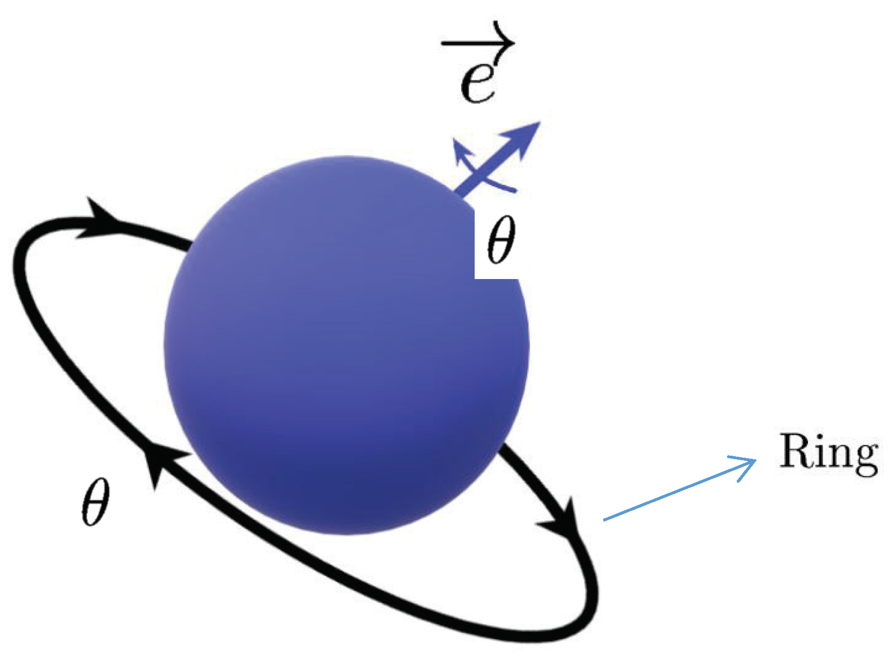
Figure 2.
The phenomenon “Gimbal Lock”.
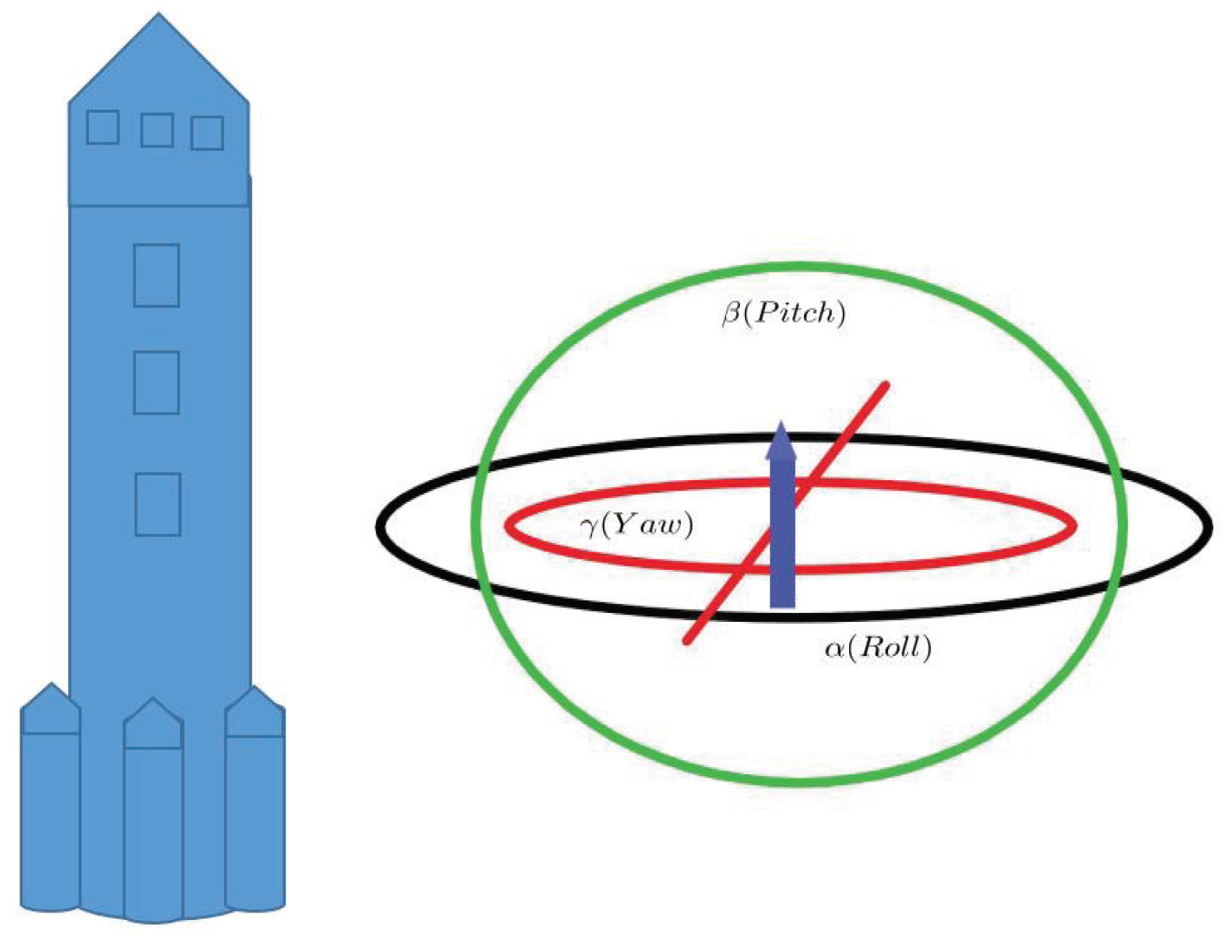
Figure 3.
The quaternion dynamic equations and the corresponding automobilism.

Figure 4.
The obstacle of the presented quaternion exponential function application.

Figure 5.
The quaternion dynamic equations and the corresponding working diagram of a warplane.
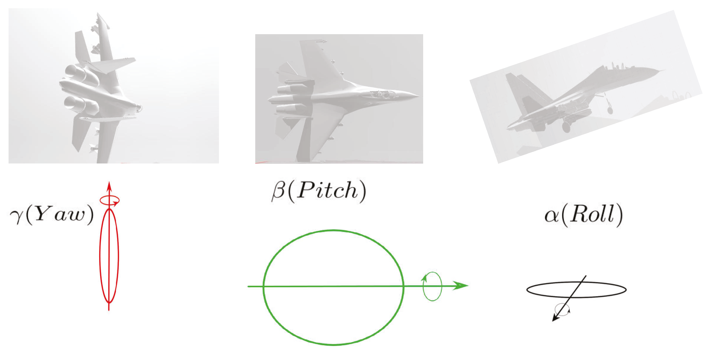
Figure 6.
The diagram of the Euler’s rotation principle.

Figure 7.
Initial state diagram of a submarine controlled by a gyroscope.
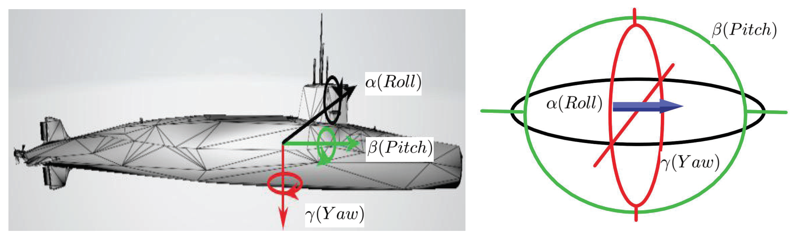
Figure 8.
A working diagram of a submarine controlled by a gyroscope.

Figure 9.
“Gimbal Lock”.
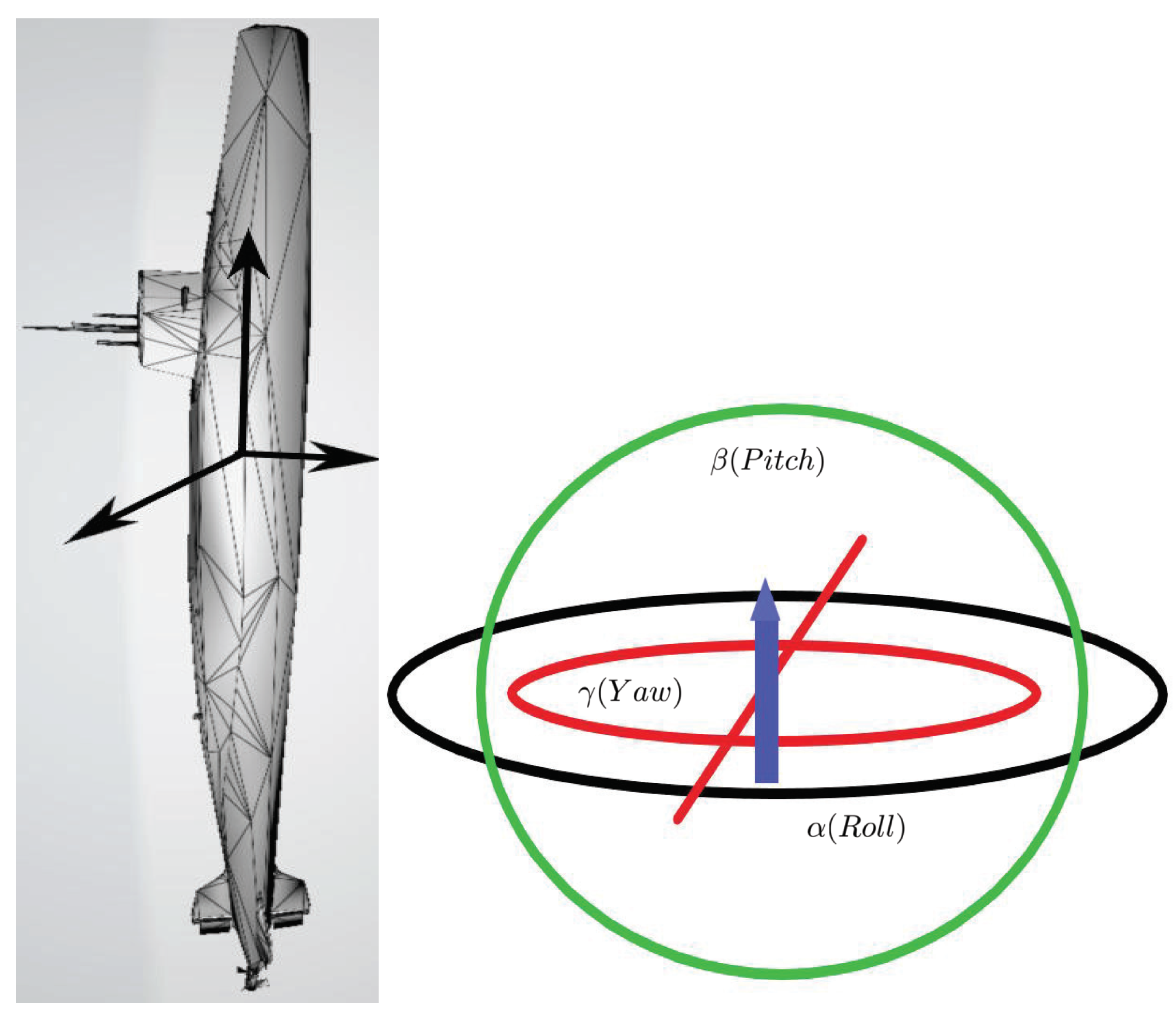
Figure 10.
The gyroscope working diagram marked on different time scales.

Figure 11.
The motion diagram of the planet rotation described by (36) which describe (the state at to the state at t by (36)).

Figure 12.
The motion diagram of submarine.
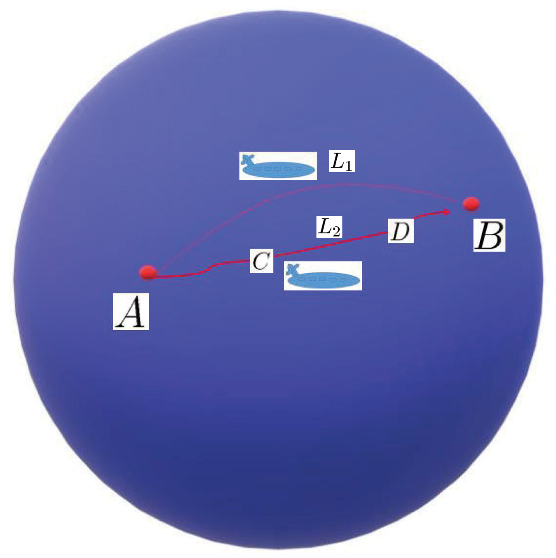
Figure 13.
The vertical evolution diagram of dynamical behavior from to under Hilger theory.

Figure 14.
The horizontal evolution diagram of dynamical behavior from to under coupled-jumping timescale theory.
Figure 14.
The horizontal evolution diagram of dynamical behavior from to under coupled-jumping timescale theory.

Figure 15.
The relation among hybrid-timescale problems, single-timescale problems, Hilger theory and coupled-jumping timescale theory.
Figure 15.
The relation among hybrid-timescale problems, single-timescale problems, Hilger theory and coupled-jumping timescale theory.
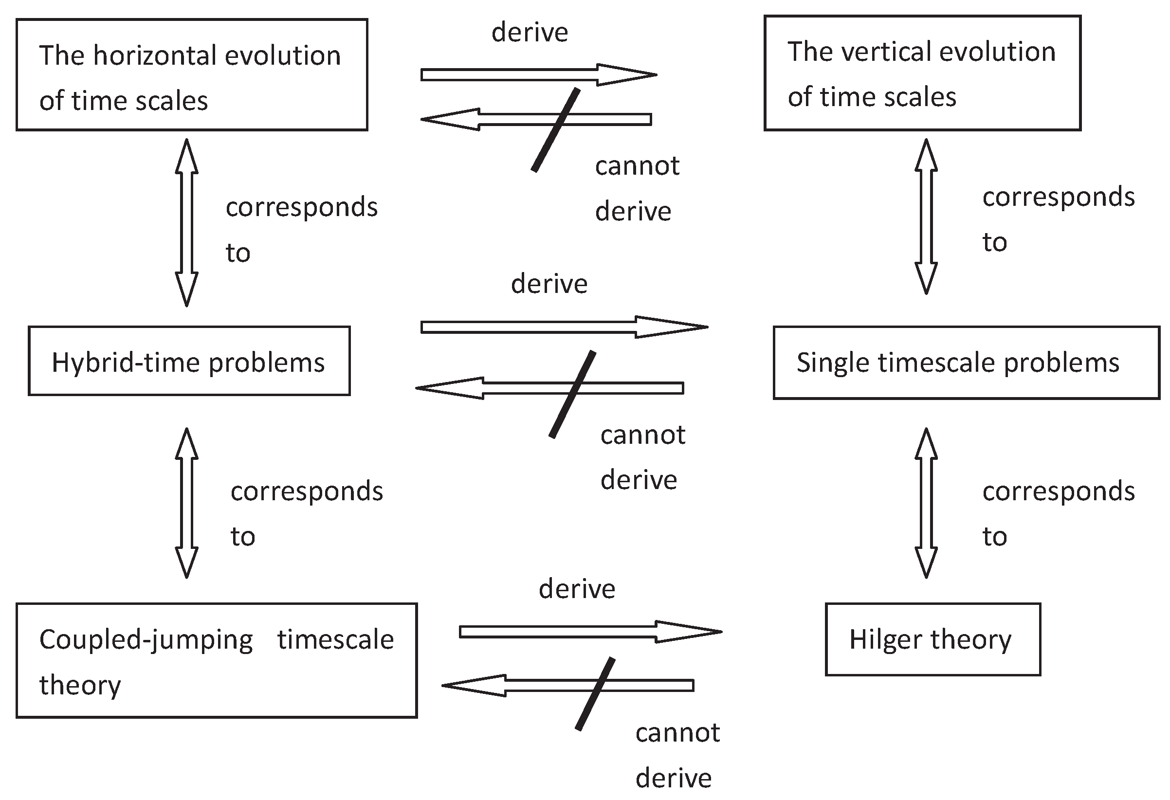
Figure 16.
Schematic diagram of all types of coupled-jumping points.

Figure 17.
The jump of coupled-jumping points in Remark 10.

Figure 18.
The jump of coupled-jumping points in Remark 13.

Figure 19.
The jump situation for the coupled-jumping points in Theorem 75.
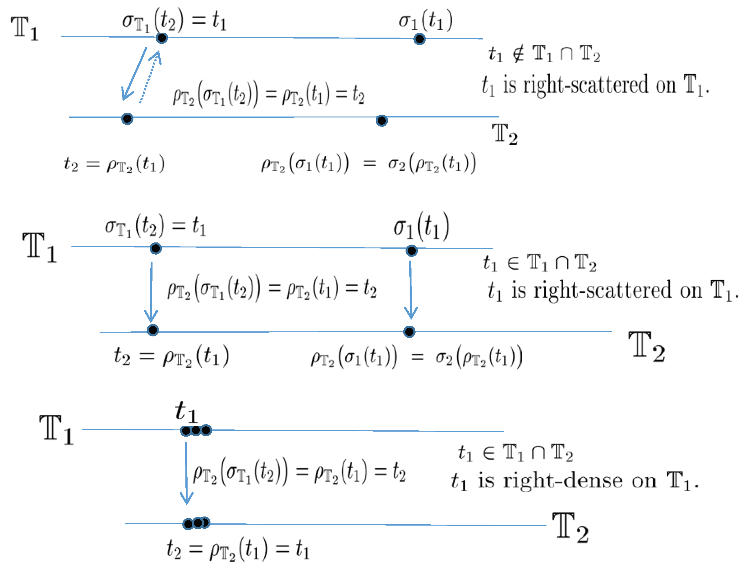

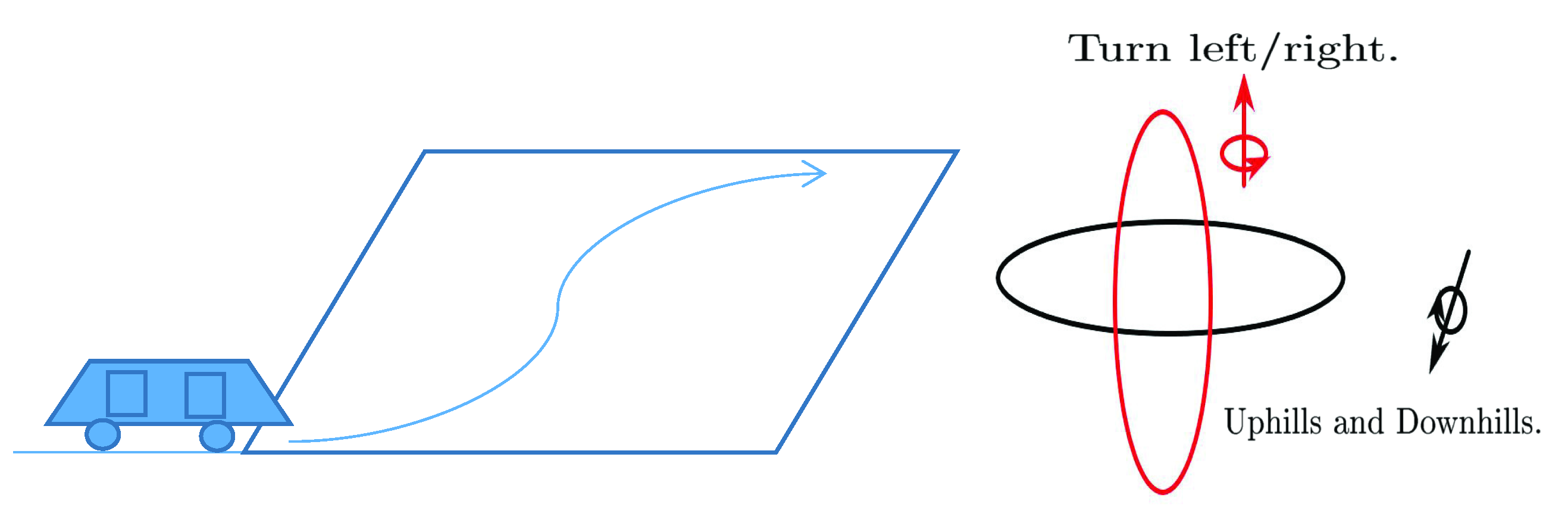
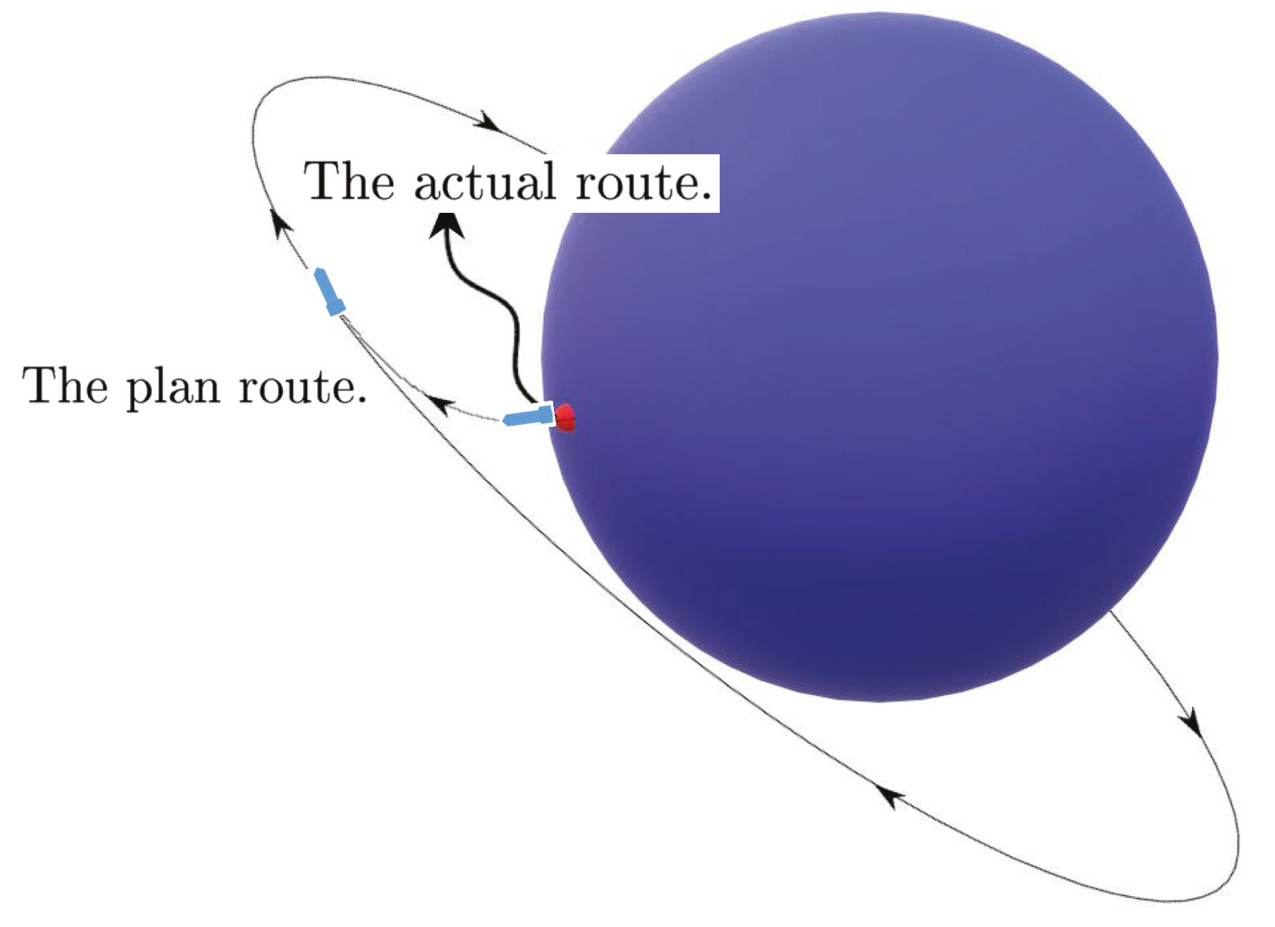
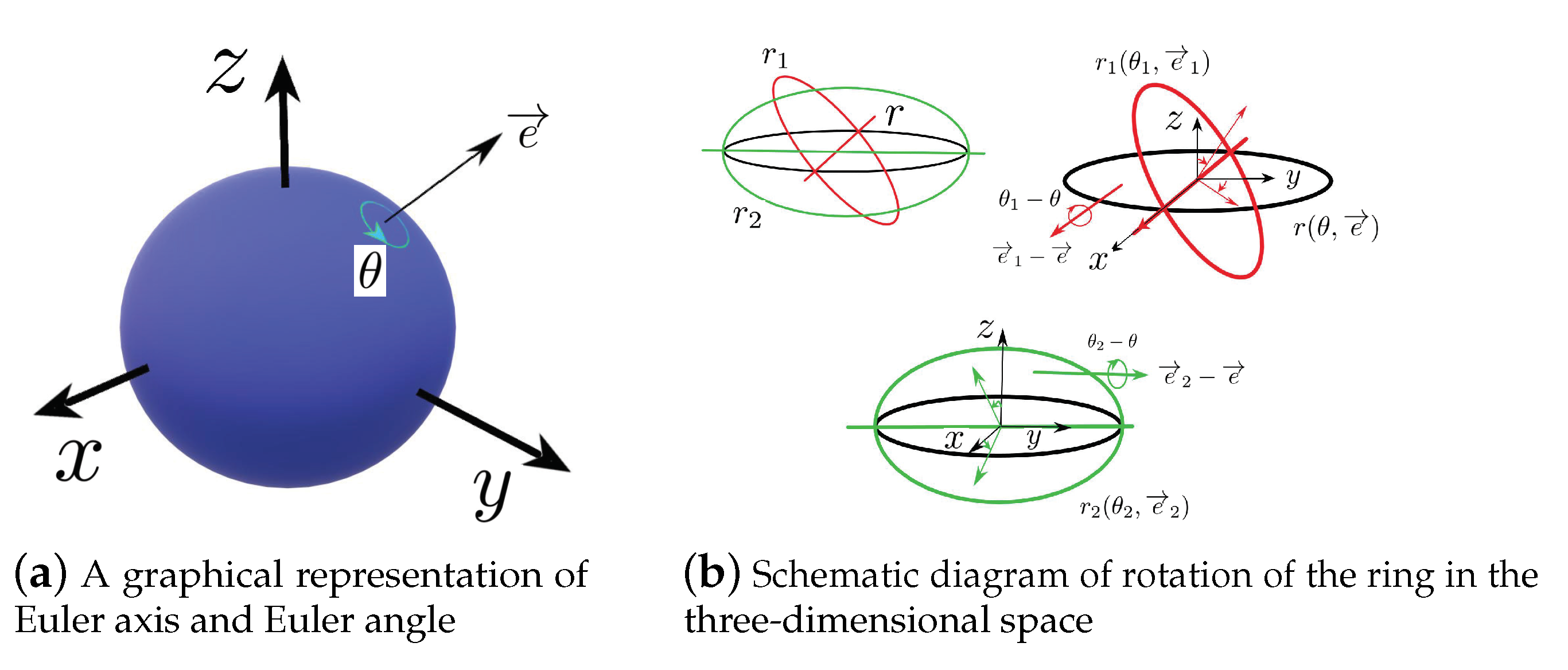
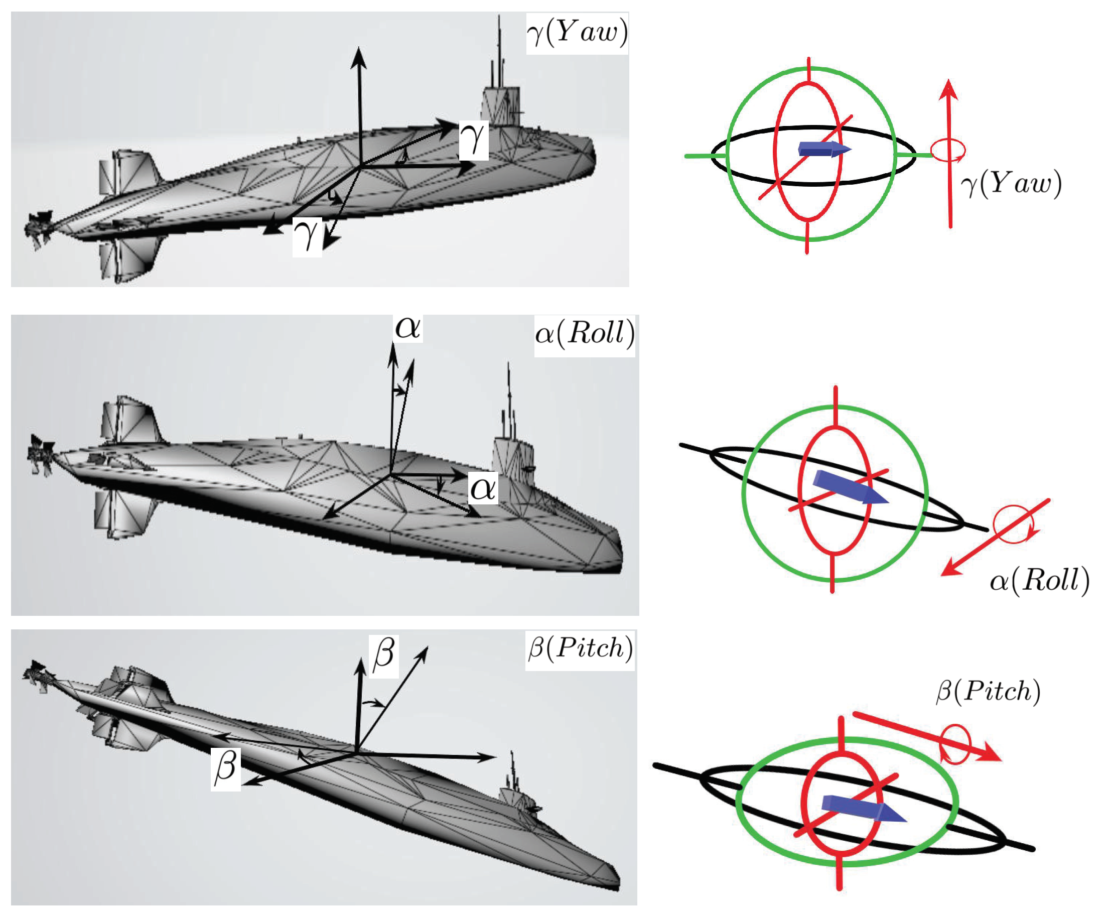
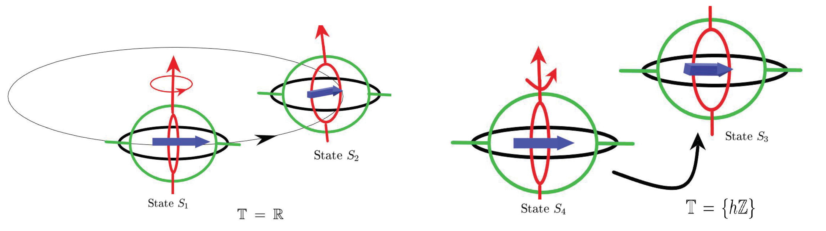
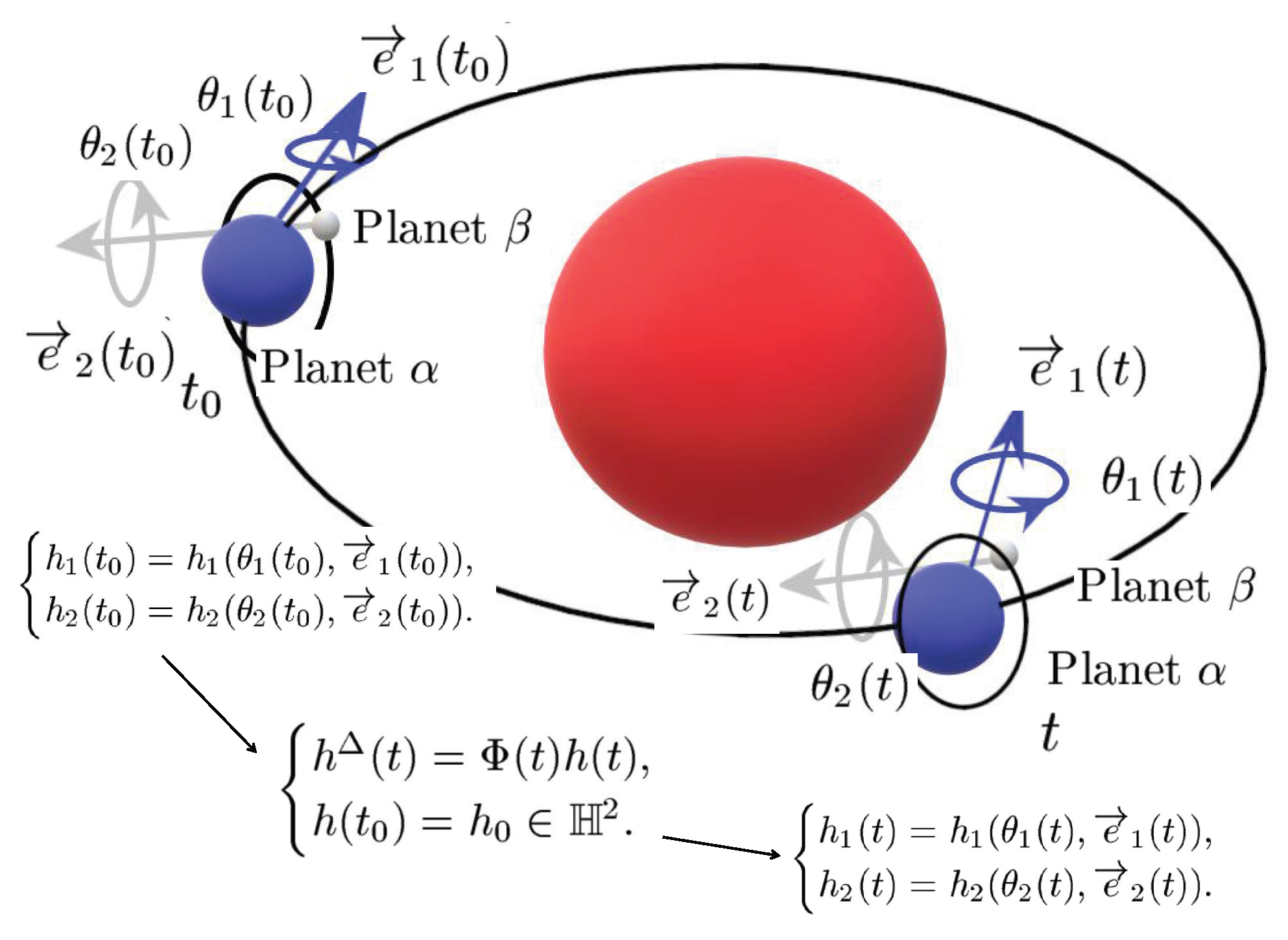
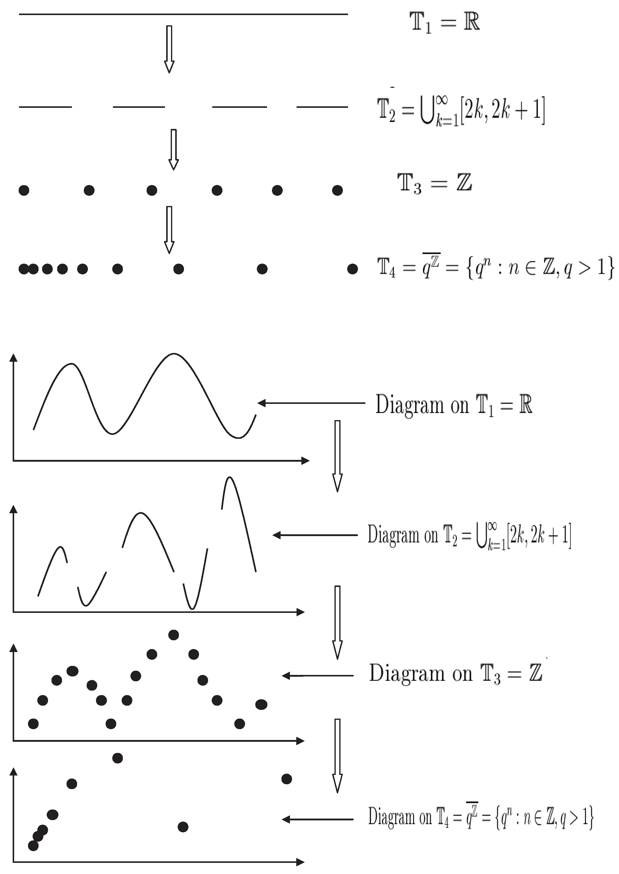
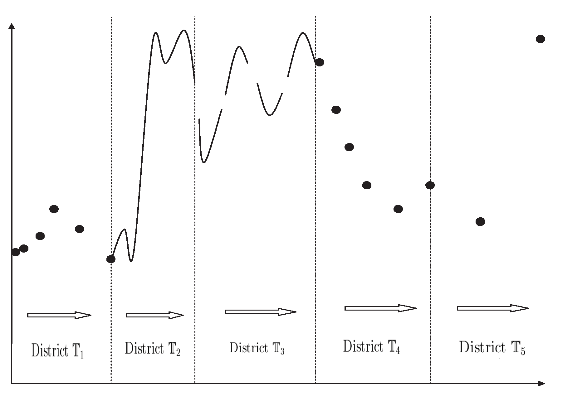
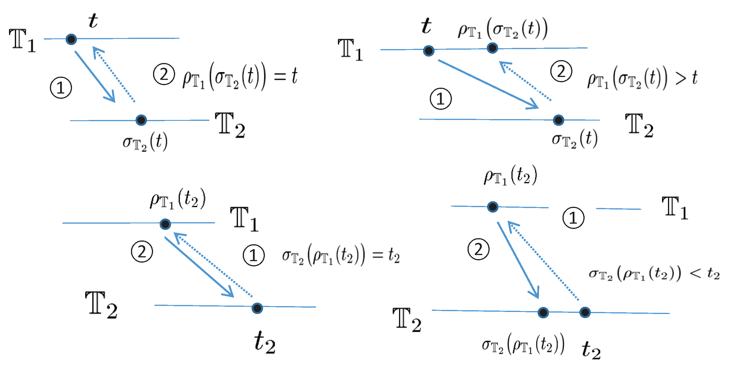
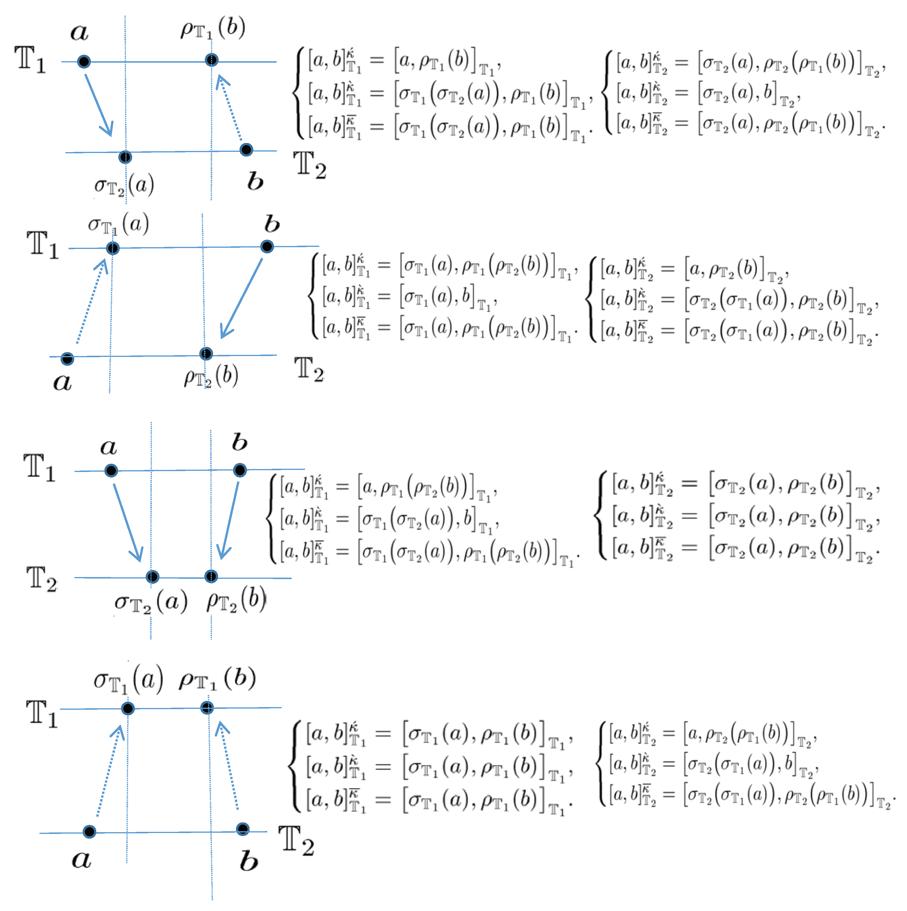
Table 1.
The solution of (38).
Table 1.
The solution of (38).
| t | |||||||||||||
| 9.7656 × 10⁻⁴ | 1 | 1 | 1 | 0 | 0 | 0 | 0 | 0 | 0 | 0 | 0 | 0 | |
| 0.0020 | 1.0010 | 1.0000 | 1.0010 | 0.0008 | 0.0068 | 0.0039 | 0.0010 | 0.0029 | 0.0010 | 0.0010 | 0.0000 | 0.0029 | |
| 0.0039 | 1.0020 | 1.0000 | 1.0020 | 0.0016 | 0.0137 | 0.0078 | 0.0020 | 0.0059 | 0.0020 | 0.0020 | 0.0000 | 0.0059 | |
| 0.0078 | 1.0039 | 1.0001 | 1.0039 | 0.0033 | 0.0273 | 0.0156 | 0.0039 | 0.0117 | 0.0039 | 0.0039 | 0.0000 | 0.0117 | |
| 0.0156 | 1.0078 | 1.0004 | 1.0079 | 0.0067 | 0.0547 | 0.0313 | 0.0079 | 0.0235 | 0.0079 | 0.0079 | 0.0001 | 0.0235 | |
| 0.0313 | 1.0156 | 1.0015 | 1.0159 | 0.0135 | 0.1094 | 0.0625 | 0.0161 | 0.0471 | 0.0161 | 0.0161 | 0.0002 | 0.0471 | |
| 0.0625 | 1.0313 | 1.0058 | 1.0322 | 0.0278 | 0.2188 | 0.1250 | 0.0332 | 0.0947 | 0.0332 | 0.0332 | 0.0010 | 0.0948 | |
| 0.1250 | 1.0626 | 1.0233 | 1.0664 | 0.0585 | 0.4375 | 0.2500 | 0.0702 | 0.1914 | 0.0702 | 0.0703 | 0.0039 | 0.1916 | |
| 0.2500 | 1.1260 | 1.0909 | 1.1406 | 0.1284 | 0.8750 | 0.5000 | 0.1550 | 0.3906 | 0.1550 | 0.1562 | 0.0156 | 0.3925 | |
| 0.5000 | 1.2578 | 1.3302 | 1.3119 | 0.2991 | 1.7500 | 1.0000 | 0.3621 | 0.8119 | 0.3621 | 0.3737 | 0.0619 | 0.8275 | |
| 1 | 1.5625 | 1.8754 | 1.7397 | 0.7385 | 3.5000 | 2.0000 | 0.8595 | 1.7397 | 0.8595 | 0.9755 | 0.2397 | 1.8634 | |
| 2 | 2.3818 | 1.1525 | 2.8415 | 1.7508 | 7.0000 | 4.0000 | 1.4496 | 3.8415 | 1.4496 | 2.2232 | 0.8415 | 4.6829 | |
| 4 | −1.3459 | 1.4651 | 4.8186 | 2.1008 | 14.0000 | 8.0000 | −2.3459 | 7.8186 | −2.3459 | 3.3462 | 1.8186 | 6.3050 | |
| 8 | −2.7662 | 3.8058 | 1.9728 | −6.8629 | 28.0000 | 16.0000 | 1.3429 | 8.9728 | 1.3429 | −4.4870 | −3.0272 | 7.8212 | |
| 16 | 7.1962 | 3.1082 | 16.9149 | 11.2118 | 56.0000 | 32.0000 | −3.4672 | 31.9149 | −3.4672 | 7.8551 | 7.9149 | 39.2751 | |
| 32 | −30.3099 | 24.5432 | 12.3935 | −19.9888 | 112.0000 | 64.0000 | −6.4997 | 43.3935 | −6.4997 | 3.6509 | −4.6065 | 27.4062 | |
| t | |||||||||||||
| 0 | 9.7656 × 10⁻⁴ | 1 | 1 | 1 | |||||||||
| 1 | 0.0020 | 1.0010 + 0.0008i + 0.0010j + 0.0010k | 1.0000 + 0.0068i + 0.0029j + 0.0000k | 1.0010 + 0.0039i + 0.0010j + 0.0029k | |||||||||
| 2 | 0.0039 | 1.0020 + 0.0016i + 0.0020j + 0.0020k | 1.0000 + 0.0137i + 0.0059j + 0.0000k | 1.0020 + 0.0078i + 0.0020j + 0.0059k | |||||||||
| 3 | 0.0078 | 1.0039 + 0.0033i + 0.0039j + 0.0039k | 1.0001 + 0.0273i + 0.0117j + 0.0000k | 1.0039 + 0.0156i + 0.0039j + 0.0117k | |||||||||
| 4 | 0.0156 | 1.0078 + 0.0067i + 0.0079j + 0.0079k | 1.0004 + 0.0547i + 0.0235j + 0.0001k | 1.0079 + 0.0313i + 0.0079j + 0.0235k | |||||||||
| 5 | 0.0313 | 1.0156 + 0.0135i + 0.0161j + 0.0161k | 1.0015 + 0.1094i + 0.0471j + 0.0002k | 1.0159 + 0.0625i + 0.0161j + 0.0471k | |||||||||
| 6 | 0.0625 | 1.0313 + 0.0278i + 0.0332j + 0.0332k | 1.0058 + 0.2188i + 0.0947j + 0.0010k | 1.0322 + 0.1250i + 0.0332j + 0.0948k | |||||||||
| 7 | 0.1250 | 1.0626 + 0.0585i + 0.0702j + 0.0703k | 1.0233 + 0.4375i + 0.1914j + 0.0039k | 1.0664 + 0.2500i + 0.0702j + 0.1916k | |||||||||
| 8 | 0.2500 | 1.1260 + 0.1284i + 0.1550j + 0.1562k | 1.0909 + 0.8750i + 0.3906j + 0.0156k | 1.1406 + 0.5000i + 0.1550j + 0.3925k | |||||||||
| 9 | 0.5000 | 1.2578 + 0.2991i + 0.3621j + 0.3737k | 1.3302 + 1.7500i + 0.8119 j + 0.0619jk | 1.3119 + 1.0000i + 0.3621j + 0.8275k | |||||||||
| 10 | 1 | 1.5625 + 0.7385i + 0.8595j + 0.9755k | 1.8754 + 3.5000i + 1.7397j + 0.2397k | 1.7397 + 2.0000i + 0.8595j + 1.8634k | |||||||||
| 11 | 2 | 2.3818 + 1.7508i + 1.4496j + 2.2232k | 1.1525 + 7.0000i + 3.8415j + 0.8415k | 2.8415 + 4.0000i + 1.4496j + 4.6829k | |||||||||
| 12 | 4 | −1.3459 + 2.1008i− 2.3459j + 3.3462k | 1.4651 + 14.0000i + 7.8186j + 1.8186k | 4.8186 + 8.0000i− 2.3459j + 6.3050k | |||||||||
| 13 | 8 | −2.7662 − 6.8629i + 1.3429j− 4.4870k | 3.8058 + 28.0000i + 8.9728j− 3.0272k | 1.9728 + 16.0000i + 1.3429j + 7.8212k | |||||||||
| 14 | 16 | 7.1962 + 11.2118i− 3.4672j + 7.8551k | 3.1082 + 56.0000i + 31.9149j + 7.9149k | 16.9149 + 32.0000i− 3.4672j + 39.2751k | |||||||||
| 15 | 32 | −30.3099 − 19.9888i− 6.4997j + 3.6509k | 24.5432 + 112.0000i + 43.3935j− 4.6065k | 12.3935 + 64.0000i− 6.4997j + 27.4062k | |||||||||
Table 2.
The solution of (41).
Table 2.
The solution of (41).
| t | |||||||||
| 0 | 0 | 1 | 1 | 0 | 0 | 0 | 0 | 0 | 0 |
| 1 | 1 | 1.0000 | 1.0000 | −14.9712 | 3.8000 | 0 | 0 | −29.9425 | 4.0000 |
| 2 | 2 | −22.1986 | 6.8883 | −14.8956 | 3.7808 | −1.2036 | 2.5922 | −12.4595 | 1.6645 |
| 3 | 3 | −24.9918 | 7.5973 | 11.8954 | −3.0193 | −0.4930 | 1.0618 | 3.6375 | −0.4859 |
| 4 | 4 | −1.4109 | 1.6119 | 16.9130 | −4.2929 | −0.0013 | 0.0028 | 0.1483 | −0.0198 |
| 5 | 5 | 3.7555 | 0.3006 | 2.3799 | −0.6041 | 0.2434 | −0.5242 | 3.3894 | −0.4528 |
| 6 | 6 | 1.5897 | 0.8503 | −0.1744 | 0.0443 | 1.1430 | −2.4619 | −5.4514 | 0.7283 |
| 7 | 7 | 4.0143 | 0.2349 | -10.3584 | 2.6292 | 0.5086 | −1.0954 | −28.1773 | 3.7642 |
| 8 | 8 | −15.2980 | 5.1367 | −18.7021 | 4.7470 | −1.0700 | 2.3046 | −19.7960 | 2.6445 |
| 9 | 9 | −28.4662 | 8.4791 | 4.3334 | −1.0999 | −0.7850 | 1.6908 | 1.8614 | −0.2487 |
| 10 | 10 | −7.7127 | 3.2114 | 19.2623 | −4.8892 | −0.0340 | 0.0732 | 1.2122 | −0.1619 |
| 11 | 11 | 4.7138 | 0.0574 | 5.7280 | −1.4539 | 0.0813 | −0.1751 | 2.0216 | −0.2701 |
| 12 | 12 | 1.0001 | 1.0000 | −0.0000 | 0.0000 | 0.9327 | −2.0088 | −0.0666 | 0.0089 |
| 13 | 13 | 4.7228 | 0.0551 | −5.8547 | 1.4860 | 0.9187 | −1.9787 | −23.2944 | 3.1119 |
| 14 | 14 | −7.9334 | 3.2675 | −19.2938 | 4.8972 | 7 − 0.7442 | 1.6029 | −25.9138 | 3.4618 |
| 15 | 15 | −28.5219 | 8.4933 | −4.0750 | 1.0343 | −1.0456 | 2.2521 | −2.3270 | 0.3109 |
| t | |||||||||
| 0 | 0 | 1 | 1 | ||||||
| 1 | 1 | 1.0000 − 14.9712i− 29.9425k | 1.0000 + 3.8000i + 4.0000k | ||||||
| 2 | 2 | −22.1986 − 14.8956i− 1.2036j− 12.4595k | 6.8883 + 3.7808i + 2.5922j + 1.6645k | ||||||
| 3 | 3 | −24.9918 + 11.8954i− 0.4930j + 3.6375k | 7.5973 − 3.0193i + 1.0618j− 0.4859k | ||||||
| 4 | 4 | −1.4109 + 16.9130i− 0.0013j + 0.1483k | 1.6119 − 4.2929i + 0.0028j− 0.0198k | ||||||
| 5 | 5 | 3.7555 + 2.3799i + 0.2434j + 3.3894k | 0.3006 − 0.6041i− 0.5242j− 0.4528k | ||||||
| 6 | 6 | 1.5897 − 0.1744i + 1.1430j− 5.4514k | 0.8503 + 0.0443i− 2.4619j + 0.7283k | ||||||
| 7 | 7 | 4.0143 −10.3584i + 0.5086j− 28.1773k | 0.2349 + 2.6292i− 1.0954j + 3.7642k | ||||||
| 8 | 8 | −15.2980 − 18.7021i− 1.0700j− 19.7960k | 5.1367 + 4.7470i + 2.3046j + 2.6445k | ||||||
| 9 | 9 | −28.4662 + 4.3334i− 0.7850j + 1.8614k | 8.4791 − 1.0999i + 1.6908j− 0.2487k | ||||||
| 10 | 10 | −7.7127 + 19.2623i− 0.0340j + 1.2122k | 3.2114 − 4.8892i + 0.0732j− 0.1619k | ||||||
| 11 | 11 | 4.7138 + 5.7280i + 0.0813j + 2.0216k | 0.0574 − 1.4539i− 0.1751j− 0.2701k | ||||||
| 12 | 12 | 1.0001 − 0.0000i + 0.9327j− 0.0666k | 1.0000 + 0.0000i− 2.0088j + 0.0089k | ||||||
| 13 | 13 | 4.7228 − 5.8547i + 0.9187j− 23.2944k | 0.0551 + 1.4860i− 1.9787j + 3.1119k | ||||||
| 14 | 14 | −7.9334 − 19.2938i− 0.7442j− 25.9138k | 3.2675 + 4.8972i + 1.6029j + 3.4618k | ||||||
| 15 | 15 | −28.5219 − 4.0750i− 1.0456j− 2.3270k | 8.4933 + 1.0343i + 2.2521j + 0.3109k | ||||||
Publisher’s Note: MDPI stays neutral with regard to jurisdictional claims in published maps and institutional affiliations. |
© 2021 by the authors. Licensee MDPI, Basel, Switzerland. This article is an open access article distributed under the terms and conditions of the Creative Commons Attribution (CC BY) license (https://creativecommons.org/licenses/by/4.0/).
Share and Cite
MDPI and ACS Style
Wang, C.; Agarwal, R.P. A Survey of Function Analysis and Applied Dynamic Equations on Hybrid Time Scales. Entropy 2021, 23, 450. https://0-doi-org.brum.beds.ac.uk/10.3390/e23040450
AMA Style
Wang C, Agarwal RP. A Survey of Function Analysis and Applied Dynamic Equations on Hybrid Time Scales. Entropy. 2021; 23(4):450. https://0-doi-org.brum.beds.ac.uk/10.3390/e23040450
Chicago/Turabian StyleWang, Chao, and Ravi P. Agarwal. 2021. "A Survey of Function Analysis and Applied Dynamic Equations on Hybrid Time Scales" Entropy 23, no. 4: 450. https://0-doi-org.brum.beds.ac.uk/10.3390/e23040450
Note that from the first issue of 2016, this journal uses article numbers instead of page numbers. See further details here.