
Thermodynamic Efficiency of Interactions in Self-Organizing Systems


1
Department of Physics and Astronomy, Macquarie University, Sydney, NSW 2109, Australia
2
Centre for Complex Systems, Faculty of Engineering, The University of Sydney, Sydney, NSW 2006, Australia
*
Author to whom correspondence should be addressed.
Entropy 2021, 23(6), 757; https://0-doi-org.brum.beds.ac.uk/10.3390/e23060757
Submission received: 21 May 2021
/
Revised: 10 June 2021
/
Accepted: 11 June 2021
/
Published: 16 June 2021
(This article belongs to the Special Issue What Is Self-Organization?)
Abstract
:The emergence of global order in complex systems with locally interacting components is most striking at criticality, where small changes in control parameters result in a sudden global reorganization. We study the thermodynamic efficiency of interactions in self-organizing systems, which quantifies the change in the system’s order per unit of work carried out on (or extracted from) the system. We analytically derive the thermodynamic efficiency of interactions for the case of quasi-static variations of control parameters in the exactly solvable Curie–Weiss (fully connected) Ising model, and demonstrate that this quantity diverges at the critical point of a second-order phase transition. This divergence is shown for quasi-static perturbations in both control parameters—the external field and the coupling strength. Our analysis formalizes an intuitive understanding of thermodynamic efficiency across diverse self-organizing dynamics in physical, biological, and social domains.
1. Introduction
Typically, self-organization is defined as a spontaneous formation of spatial, temporal, and spatiotemporal structures or functions in a system comprising multiple interacting components. Importantly, a self-organizing process is assumed to develop in the absence of specific external controls, as pointed out by Haken [1]:
A system is self-organizing if it acquires a spatial, temporal or functional structure without specific interference from the outside. By ‘specific’ we mean that the structure or functioning is not impressed on the system, but that the system is acted upon from the outside in a non-specific fashion. For instance, the fluid which forms hexagons is heated from below in an entirely uniform fashion, and it acquires its specific structure by self-organization.
To explain structures that spontaneously self-organize when energy or matter flows into a system typically describable by many variables, Haken employed the notion of order parameters (degrees of freedom) and control parameters [1,2]: slowly varying a relevant control parameter, such as temperature of a ferromagnetic material, may induce an abrupt change—a phase transition—in an observable order parameter, such as the net magnetization. The emergence of global order in complex systems is most striking at criticality, when the characteristic length and dynamical time scales of the system diverge. A phase transition is usually accompanied by global symmetry breaking. Crucially, in the more organized (coherent) phase of the system dynamics, the global behavior of the system can be described by only a few order parameters, that is, the system becomes low-dimensional as some dominant variables “enslave” others.
In physical systems, the local interactions are usually determined by physical laws, e.g., interactions among fluid molecules or crystal ions, while the interactions within a biological organism may evolve over generations under environmental selection pressures, bringing survival benefits. The role of locally interacting particles contributing to self-organizing pattern formation in biological systems has been captured in a definition offered by Camazine et al. [3]:
Self-organization is a process in which pattern at the global level of a system emerges solely from numerous interactions among the lower-level components of the system. Moreover, the rules specifying interactions among the system’s components are executed using only local information, without reference to the global pattern.
These definitions concur with many other approaches to formalize self-organization, highlighting three important aspects [4,5]: (i) a system dynamically advances to a more organized state, while exchanging energy, matter, and/or information with the environment, but without a specific external ordering influence; (ii) the interacting system components have only local information, and thus exchange only local information, but exhibit long-range correlations; (iii) the increase in organization can be observed as a more coherent global behavior.
In general, as the state of a complex system evolves, its configurational entropy changes. The reduction (or increase) in the configurational entropy occurs at the expense of work extracted or carried out on the system and the heat exported to the environment. Thus, a thermodynamic analysis of the interactions in self-organizing systems aims to quantify the work, heat, and energy exchange between the system and the environment. One can reasonably expect that self-organization is most thermodynamically efficient in the vicinity of the critical points, i.e., at criticality, one may expect that a smaller amount of work extracted/done on a system can result in a larger change of the configurational entropy. Indeed, it has been conjectured before that a system in a self-organized low-dimensional phase with fewer available configurations (i.e., describable by just a few order parameters and exhibiting macroscopic stability) may be more efficient than the system in a high-dimensional disorganized phase with more configurations.
To formalize this conjecture, Kauffman proposed a succinct principle behind the higher efficiency of self-organized systems—the generation of constraints during the release of energy—the constrained release channels energy to perform some useful work, which can propagate and be used again to create more constraints, releasing further energy and so on [6]. Following a similar characterization, Carteret et al. [7] have shown that available power efficiency is maximized at critical Boolean networks. The question of thermodynamic efficiency has also been proposed and studied in the context of cellular information-processing, from the perspective of how close life has evolved to approach maximally efficient computation [8,9]. Furthermore, a recent thermodynamic analysis of a model of active matter demonstrated that the efficiency of the collective motion diverges at the transition between disordered and coherent collective motion [10]. However, the precise nature of the divergence of the efficiency of collective motion, and its relation to the critical exponents describing the system behavior in the vicinity of the phase transitions remained unclear, due to the lack of analytical expressions for the corresponding configurational probability distributions.
In this work, we study the thermodynamic efficiency of interactions within a canonical self-organizing system, aiming to clearly differentiate between phases of system dynamics, and identify the regimes when efficiency is maximal. This measure is expressed by contrasting (i) the change of organization attained within the system (i.e., change in the created order or predictability) with (ii) the thermodynamic work involved in driving such a change. We demonstrate that the maximal efficiency is indeed achieved at the critical regime, i.e., during the phase transition, rather than at the macroscopically stable low-dimensional phase per se. The reasons for the maximal efficiency exhibited by systems during self-organization, i.e., at a critical regime, are articulated precisely in terms of the increased order (or the reduction of Shannon entropy) related to the amount of work carried out during the transition. This measure is defined for specific configurational changes (perturbations), rather than states or regimes—in line with the point made by Carteret et al. [7] that the maximization of power efficiency occurs at a finite displacement from equilibrium.
In studying the thermodynamic efficiency, we select an abstract statistical–mechanical model (Curie-Weiss model of interacting spins in a fully connected graph)—one of the simplest models exhibiting a second-order phase transition—from the widely applicable mean-field universality class. We analytically evaluate dynamics of this model in the vicinity of a phase transition, prove that the thermodynamic efficiency has a power law divergence at the critical point, and compute its critical exponent.
2. Framework
Consider a statistical–mechanical system in thermodynamic equilibrium, where are intensive thermodynamic quantities that act as control parameters that can be changed externally. For example, in an n-vector spin model, the control parameter is a linear combination of externally applied fields. A perturbation in the control parameter, , will result in a change in thermodynamic potentials in the system, including its entropy and energy. Following [10], we formalize the thermodynamic efficiency of interactions as
where and are the change in entropy and the work done/extracted on the system due to the perturbation . Entropy S is a configurational entropy, and thus, quantifies the reduction (increase) of uncertainty in the state of the system that we gain per unit of work done. A high value of signifies that it is energetically easy to create order (reduce the configurational uncertainty) in the system by changing a control parameter, whereas a low value of indicates that a lot of work is needed to change the order in the system.
In practice, to evaluate , we need to specify the perturbation protocol. A change in control parameters moves the system out of thermal equilibrium, and we need to compute the amount of work done/extracted as the system relaxes back to its equilibrium state. Thus, depends on how we perturb the system, and on the master equation that describes the relaxation of the system back to its equilibrium state. In what follows, we will consider the case of a quasi-static perturbation protocol, i.e., we assume that the perturbation is sufficiently slow that the system effectively adjusts instantaneously to its new equilibrium state. Helmholtz free energy is the most useful thermodynamic potential for analyzing the quasi-static protocols at constant temperature. Helmholtz free energy is related to the internal energy U and entropy S via equation
where T. To a first order in , the change in internal energy, entropy, and free energy induced by varying the control parameters are , , and . In a quasi-static process, the change in free energy can be identified with the work done on the system , and the entropy change in the system balances the entropy exported to the environment . Thus, for a quasi-static protocol, the thermodynamic efficiency reduces to
In the case when the variation of control parameter is one-dimensional , Equation (2) simplifies to
Equation (3) applies for general quasi-static processes. When the system is close to a critical point of a phase transition, the expression for can further be simplified using the following argument. Let be an extensive quantity conjugate to X
Entropy is related to free energy via , and thus, the derivative of S with respect to X is
Thus, in terms of the extensive variable conjugate to the control parameter, the efficiency given by Equation (3) can be expressed as
If is an order parameter of a phase transition, then, near the critical point we have , where is the critical temperature, is the critical exponent, and a is nonuniversal proportionality constant. Upon substitution of this expression for into (5), the constant a cancels and we obtain
Equation (6) expresses the divergence of solely in terms of universal exponent . This result explains why in many thermodynamic models, the efficiency of self-organization is expected to peak near the critical point.
In many complex systems, there may not exist a readily available physical model expressed in terms of a Hamiltonian and the expression for the order parameter may not be evident. Nevertheless, if there is a record of samples of the states of the system, then one may still use Equation (3) to compute the efficiency of self-organization. The reason is that all of the thermodynamic quantities in (3), expressed in terms of Gibbs probability distribution, have a clear information-theoretic interpretation. Entropy S is directly proportional to the Shannon entropy H, . The free energy F is related to the Fisher information via equation , with the Fisher information quantifying the sensitivity of the probability distribution to the change in the control parameter, .
There are several interpretations of the Fisher information relevant to critical dynamics and scale dependence: is equivalent to the thermodynamic metric tensor, the curvature of which diverges at phase transitions; further, is proportional to the derivatives of the corresponding order parameters with respect to the collective variables [11,12,13,14,15,16]. The statistical physics of linear response theory [17] considers similar phenomena. In particular, it is well-known that Fisher information is proportional to isothermal susceptibility [15]. In addition, measures the size of the fluctuations in the collective variables around equilibrium [17,18]. In this work, we extend this approach, based on linear response theory, to the analysis of thermodynamic efficiency.
Substituting into Equation (3) gives
Equation (7) expresses the thermodynamic efficiency of interaction during configurational perturbations in terms of information-theoretic quantities of entropy and Fisher information.
Equation (7) was derived and used in [10] in the thermodynamic analysis of collective motion (e.g., swarming) exhibiting a kinetic phase transition. Crosato et al. [10] computed the efficiency from the distribution , estimated via sampling produced by numerical simulations of the model, consequently yielding estimates of H and . It was then demonstrated that diverges at the critical point where the swarm transitions from disordered to coherent motion.
The notion of thermodynamic efficiency was also applied to the analysis of urban transformations [19], driven by quasi-static changes in the social disposition: a control parameter characterizing the attractiveness of different areas. The thermodynamic efficiency of urban transformations was defined as the reduction of configurational entropy resulting from the expenditure of work. In the socioeconomic context of urban dynamics, it expressed the ratio of the gained predictability of income flows to the amount of work required to change the social disposition. Importantly, the efficiency was shown to peak at a critical transition, separating dispersed and polycentric phases of urban dynamics [19].
Similarly, Harding et al. [20] considered thermodynamic efficiency of quasi-static epidemic processes, defined for a value of some control parameter (e.g., the infection transmission rate), as the ratio of the reduction in uncertainty to the expenditure of work needed to change the parameter. On the one hand, this could be the efficiency of an intervention process consuming work in order to reduce the transmission rate. On the other hand, the efficiency can be defined in terms of the pathogen emergence—a process that increases the transmission rate, and in doing so extracts the work. Irrespective of the interpretation, the efficiency was shown to peak at the epidemic threshold [20].
Our contribution builds on this research, showing that according to Equation (6), the divergence of the efficiency of self-organization is generally expected to occur at a second-order phase transition. In the following section, we illustrate this result by explicitly computing in a canonical model exhibiting paramagnetic to ferromagnetic phase transition, showing that the efficiency of self-organization peaks at the critical point when the control parameter is either the coupling strength between the spins or the external magnetic field.
3. Example: Curie–Weiss Model
The energy of a wide variety statistical–mechanical systems, including spin glasses, can be expressed as a linear combination of functions of the microscopic state .
where defines the control parameters of the system and . We are working with a canonical ensemble, where the system is in contact with a heat bath in thermal equilibrium and the average energy is fixed. In this case, the probability of finding the system in configuration is given by the Gibbs measure
where is the partition function. The free energy of the system is given by . The free energy can be used to compute any thermodynamic quantity, in particular, the expectations of are given by
For an interacting statistical–mechanical system in thermal equilibrium, there is a one-to-one map between the the set of control parameters and [21]; thus, we will refer to as a order parameter conjugate to the control parameter . Phase transitions are often accompanied by divergences in one or more order parameters or their derivatives.
In the rest of the paper, we will focus on computing for a system governed by a specific energy function of the form (8)—the Curie–Weiss (CW) model. The CW model is a model of ferromagnetism, where each spin interacts with all other spins via pairwise interactions, and for this reason, it is also known as the fully connected Ising model. This model exhibits a second-order phase transition at a finite critical temperature . In the vicinity of the critical point, the analytic expression to all of the thermodynamic quantities are known, which enables the derivation of the analytic expression for . The phase transition from ferromagnetic to paramagnetic states in the Curie–Weiss model belongs to the mean field universality class.
Let N spins be assigned to sites . A configuration of the system is given by . The energy function for the system containing pairwise interactions between spins and in the presence of an external magnetic field B is given by
where the sum over ) runs over all of the . The scaling in front of the spin–spin interaction term is to yield an extensive free energy. In this model, the control parameters are , which denote exchange interaction strength and externally applied magnetic field, respectively. The probability of finding the system in configuration is given by the Gibbs measure
where and is a partition function for the N-spin system. The free energy of the N spin system is given by . The thermodynamic limit is obtained by taking . In the thermodynamic limit, the free energy density can have the following analytic expression [22]:
with
Here, y is defined as a solution to the equation
The average magnetization per spin is the order parameter conjugate to the magnetic field and is given by ; thus, the equation of state is . The phase diagram can be constructed by analyzing the equation of state. The critical point of a second-order phase transition occurs at and . When and , there is only one stable solution of the equation of state, which is . When and , there are three solutions: one unstable solution and two stable solution , where is found by numerically solving the equation . Thus, at and at the critical temperature , the system transitions from a paramagnetic disordered state where to a ferromagnetic ordered state where . This transition is of second order, since the second derivatives of f with respect to both B and are discontinuous at .
Having reviewed the phase change behavior of the CW model, we will now evaluate the thermodynamic efficiency associated with varying the magnetic field B along a quasi-static protocol. The entropy density is related to the free energy density via equation
Using Equations (2) and (13)–(16), one can compute the efficiency of self-organization resulting from variation of one or more control parameters B, J, or .
3.1. Varying External Field, B
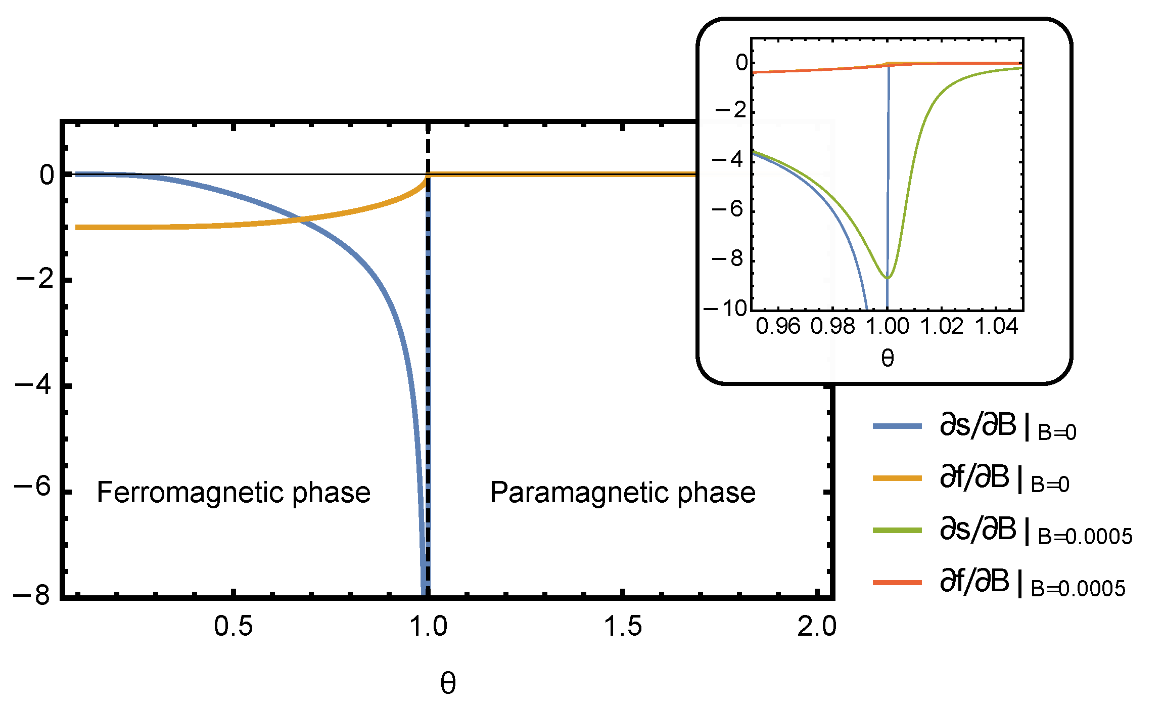
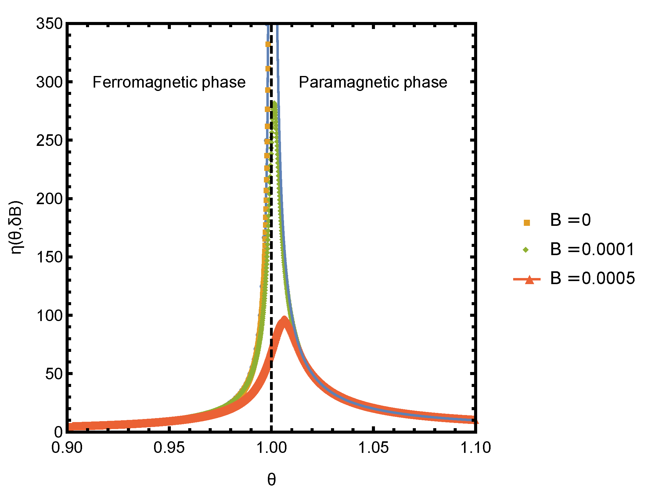
Since Equation (15) does not have a closed form solution for , it has to be solved numerically. Thus, for a general choice of parameters of the Curie–Weiss model, the efficiency needs to be evaluated numerically. The plots of derivatives of free energy and entropy densities computed numerically by solving Equation (15) are shown in Figure 1. The thermodynamic efficiency is the ratio of these two derivatives, , which is plotted in Figure 2. As expected, the efficiency peaks near the critical point of the phase transition. In the rest of this section, we focus on the behavior of in the vicinity of the critical point, where it is possible to obtain an analytic solution for all thermodynamic quantities and study their scaling behavior.
Near the critical point of the paramagnetic to ferromagnetic phase transition, the average magnetization is small, and thus, equation of state (15) can be approximated by a low-order Taylor expansion in y. Keeping up to , the equation of state is
where , . In the case of zero magnetic field, , the solution of (17) is
where t is the reduced temperature and . Equation (17) produces the well-known mean field scaling law for magnetization for , with the critical exponent . Using Equation (6), we arrive at for .
In the paramagnetic case , , both and are zero and, consequently, the efficiency appears to be undefined as it is a ratio of these derivatives. Nevertheless, in the paramagnetic regime, the derivatives of free energy and entropy can be made finite by either adding a small external magnetic field or by considering a finite size system. Here, we will consider the efficiency in the presence of constant magnetic field , which can be made arbitrarily small. In the presence of the external field and when , the equation of state (17) simplifies to , since the term is negligible. Thus, in this regime, and f can now be evaluated using Equations (13) and (14). From f, we compute and , then Taylor expands to the leading order in B to obtain
Now, we can evaluate scaling behavior of the thermodynamic efficiency around the critical point:
A plot of in the vicinity of the critical point for several small values of bias field is shown in Figure 2. The curves were obtained by numerically solving for y and numerically computing the derivative of f and s. The scaling prediction agrees very well with the numerical results. The deviations at finite and very close to the critical point are expected, as the scaling was obtained by neglecting the term in Equation (17), which is not small around .
3.2. Varying Coupling Strength, J
We now consider computing , when J is used as a control parameter. In this case, the relevant order parameter is , which quantifies the interaction energy between pairs of spins. The spins will spontaneously align at a critical value of coupling strength , and the efficiency is expected to peak near the critical point.
Near the critical point, there is a closed form expression for y, and thus, we can derive the scaling relation between and the reduced coupling strength . For the ferromagnetic case , inserting Equation (18) into the expressions for the free energy and entropy, taking derivatives with respect to and then Taylor-expanding in to the lowest orders yields
The order parameter conjugate to can be defined as , which, according to Equation (22), is linearly proportional to , i.e., with . Using Equation (6) with critical exponent , we immediately arrive at for .
In the paramagnetic case, the magnetization is zero in the absence of the external magnetic field and the efficiency of interactions is undefined since . However, in the presence of small bias magnetic field , can be computed, since in that case, . Taylor-expanding and computed with this expression for y to the lowest orders in gives
Using Equations (22)–(25), we can compute the efficiency of interactions in the vicinity of the critical point:
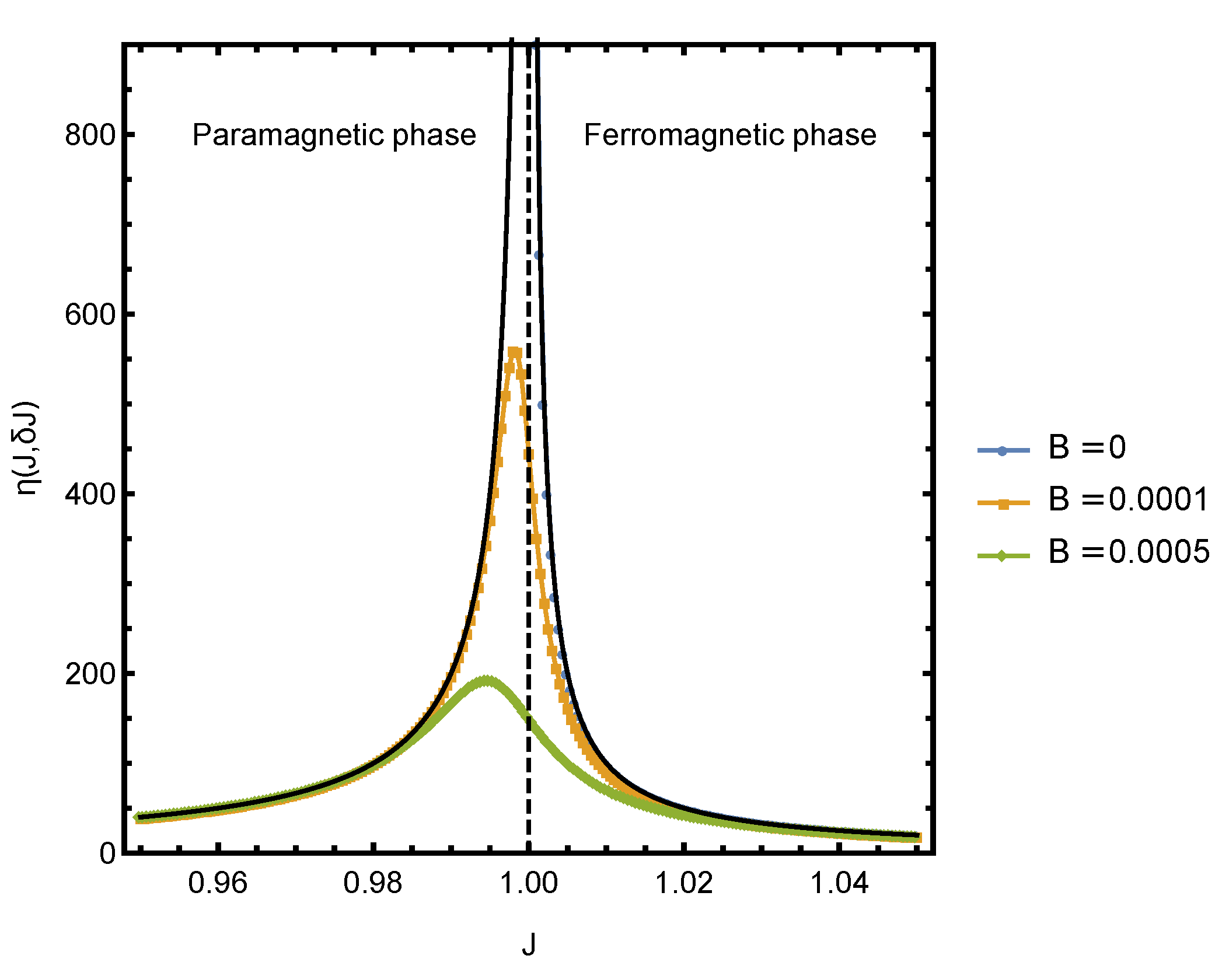
Figure 3 shows the plot of in the vicinity of the critical point for several small values of bias field . The dotted curves were obtained by numerically solving for y and computing the derivative of f and s. The solid black lines indicate the scaling, which agrees very well with the numerical results.
4. Conclusions
The increasing interest in developing a comprehensive thermodynamic framework for studying complex system, including the process of self-organization, is driven by several recent developments: theoretical advances in stochastic thermodynamics [23] that enable rigorous quantitative analysis of small and mesoscale systems; technological advances that enable measurement of thermodynamic quantities of such systems [24,25,26]; and a fusion of information-theoretic, computation-theoretic, and statistical–mechanical approaches for analyzing energy-efficiency of information processing devices [27].
We modeled the thermodynamic efficiency of interactions in a canonical self-organizing system, by quantifying the change in the order in the system per unit of work done/extracted due to the changes in control parameters. We have shown that this quantity peaks at the critical regime, by explicitly deriving it for the exactly solvable Curie–Weiss model—a paradigmatic model of second-order phase transitions. Quasi-static perturbation in both control parameters, the interaction strength between spins, and the externally applied magnetic field have been considered, and both protocols have been shown to lead to divergence of the efficiency of interactions at criticality.
These results contribute to a common understanding of thermodynamic efficiency across multiple examples of self-organizing dynamics in physical, biological, and social domains. These phenomena include transitions from disordered to coherent collective motion [10,28,29,30,31,32,33], chaos-to-order transitions in genetic regulatory networks modeled as random Boolean networks [7,14], evolutionary potential games on lattices and graphs [34], synchronization in networks of coupled oscillators near “the edge of chaos” [35,36], transitions across epidemic thresholds during contagions [20,37,38,39], and critical dynamics of urban evolution [19,40,41], among many others. Self-organizing criticality (SOC) [42] is a related but distinct phenomenon, as we are not attempting to reveal the mechanisms of self-organization towards critical regimes, focusing instead on defining and determining the thermodynamic efficiency of interactions in a representative self-organizing system.
Our work aims to support systematic thermodynamic studies of self-organization in complex systems, potentially extending the analysis to the protocols that drive the system out of equilibrium. We believe that an approach to self-organization incorporating thermodynamic efficiency will help in clarifying the fundamental relationship between the structure of a complex system and its collective behavior and functions [43], as well as support efforts to systematically control and guide the dynamics of complex systems [44,45].
Author Contributions
Conceptualization, R.N. and M.P.; methodology, R.N. and M.P.; formal analysis, R.N.; investigation, R.N. and M.P.; writing—original draft preparation, R.N.; writing—review and editing, R.N. and M.P.; visualization, R.N.; supervision, M.P.; project administration, M.P. and R.N. All authors have read and agreed to the published version of the manuscript.
Funding
This research received no external funding.
Institutional Review Board Statement
Not applicable.
Informed Consent Statement
Not applicable.
Data Availability Statement
Not applicable.
Conflicts of Interest
The authors declare no conflict of interest.
References
- Haken, H. Information and Self-Organization: A Macroscopic Approach to Complex Systems; Springer: Berlin/Heidelberg, Germany, 1988. [Google Scholar]
- Haken, H. Synergetics, an Introduction: Nonequilibrium Phase Transitions and Self-Organization in Physics, Chemistry, and Biology, 3rd ed.; Springer: New York, NY, USA, 1983. [Google Scholar]
- Camazine, S.; Deneubourg, J.L.; Franks, N.R.; Sneyd, J.; Theraulaz, G.; Bonabeau, E. Self-Organization in Biological Systems; Princeton University Press: Princeton, NJ, USA, 2001. [Google Scholar]
- Bonabeau, E.; Theraulaz, G.; Deneubourg, J.L.; Camazine, S. Self-organisation in social insects. Trends Ecol. Evol. 1997, 12, 188–193. [Google Scholar] [CrossRef] [Green Version]
- Polani, D. Measuring self-organization via observers. In Advances in Artificial Life, Proceedings of the 7th European Conference on Artificial Life (ECAL), Dortmund, Germany, 14–17 September 2003; Banzhaf, W., Christaller, T., Dittrich, P., Kim, J.T., Ziegler, J., Eds.; Springer: Berlin/Heidelberg, Germany, 2003; pp. 667–675. [Google Scholar]
- Kauffman, S.A. Investigations; Oxford University Press: Oxford, UK, 2000. [Google Scholar]
- Carteret, H.; Rose, K.; Kauffman, S. Maximum Power Efficiency and Criticality in Random Boolean Networks. Phys. Rev. Lett. 2008, 101, 218702. [Google Scholar] [CrossRef] [Green Version]
- Barato, A.; Hartich, D.; Seifert, U. Efficiency of cellular information processing. New J. Phys. 2014, 16, 103024. [Google Scholar] [CrossRef] [Green Version]
- Kempes, C.; Wolpert, D.; Cohen, Z.; Pérez-Mercader, J. The thermodynamic efficiency of computations made in cells across the range of life. Philos. Trans. R. Soc. Math. Phys. Eng. Sci. 2017, 375. [Google Scholar] [CrossRef] [PubMed]
- Crosato, E.; Spinney, R.E.; Nigmatullin, R.; Lizier, J.T.; Prokopenko, M. Thermodynamics and computation during collective motion near criticality. Phys. Rev. E 2018, 97, 012120. [Google Scholar] [CrossRef] [PubMed] [Green Version]
- Brody, D.; Rivier, N. Geometrical aspects of statistical mechanics. Phys. Rev. E 1995, 51, 1006–1011. [Google Scholar] [CrossRef] [PubMed]
- Brody, D.; Ritz, A. Information geometry of finite Ising models. J. Geom. Phys. 2003, 47, 207–220. [Google Scholar] [CrossRef]
- Janke, W.; Johnston, D.; Kenna, R. Information geometry and phase transitions. Phys. Stat. Mech. Appl. 2004, 336, 181–186. [Google Scholar] [CrossRef] [Green Version]
- Wang, X.; Lizier, J.; Prokopenko, M. Fisher Information at the Edge of Chaos in Random Boolean Networks. Artif. Life 2011, 17, 315–329. [Google Scholar] [CrossRef] [PubMed]
- Prokopenko, M.; Lizier, J.; Obst, O.; Wang, X. Relating Fisher information to order parameters. Phys. Rev. E 2011, 84, 041116. [Google Scholar] [CrossRef] [Green Version]
- Machta, B.B.; Chachra, R.; Transtrum, M.K.; Sethna, J.P. Parameter Space Compression Underlies Emergent Theories and Predictive Models. Science 2013, 342, 604–607. [Google Scholar] [CrossRef] [Green Version]
- Kubo, R.; Toda, M.; Hashitsume, N. Statistical Physics II: Nonequilibrium Statistical Mechanics, 2nd ed.; Springer: Berlin/Heidelberg, Germany, 1991. [Google Scholar]
- Crooks, G. Measuring Thermodynamic Length. Phys. Rev. Lett. 2007, 99, 100602. [Google Scholar] [CrossRef] [Green Version]
- Crosato, E.; Nigmatullin, R.; Prokopenko, M. On critical dynamics and thermodynamic efficiency of urban transformations. R. Soc. Open Sci. 2018, 5, 180863. [Google Scholar] [CrossRef] [PubMed] [Green Version]
- Harding, N.; Nigmatullin, R.; Prokopenko, M. Thermodynamic efficiency of contagions: A statistical mechanical analysis of the SIS epidemic model. Interface Focus 2018, 8, 20180036. [Google Scholar] [CrossRef] [PubMed]
- Wei, B.B. Insights into phase transitions and entanglement from density functional theory. New J. Phys. 2016, 18, 113035. [Google Scholar] [CrossRef] [Green Version]
- Kochmanski, M.; Paszkiewicz, T.; Wolski, S. Curie-Weiss magnet—A simple model of phase transition. Eur. J. Phys. 2013, 34, 1555. [Google Scholar] [CrossRef] [Green Version]
- Seifert, U. Stochastic thermodynamics, fluctuation theorems, and molecular machines. Rep. Prog. Phys. 2012, 75, 126001. [Google Scholar] [CrossRef] [PubMed] [Green Version]
- Bérut, A.; Petrosyan, A.; Ciliberto, S. Information and thermodynamics: Experimental verification of Landauer’s Erasure principle. J. Stat. Mech. Theory Exp. 2015, 2015, P06015. [Google Scholar] [CrossRef]
- Nisoli, C. Write it as you like it. Nat. Nanotechnol. 2018, 13, 5–6. [Google Scholar] [CrossRef]
- Lao, Y.; Caravelli, F.; Sheikh, M.; Sklenar, J.; Gardeazabal, D.; Watts, J.D.; Albrecht, A.M.; Scholl, A.; Dahmen, K.; Nisoli, C.; et al. Classical topological order in the kinetics of artificial spin ice. Nat. Phys. 2018, 14, 723–727. [Google Scholar] [CrossRef]
- Wolpert, D.H. The stochastic thermodynamics of computation. J. Phys. A 2019, 52, 193001. [Google Scholar] [CrossRef] [Green Version]
- Grégoire, G.; Chaté, H. Onset of Collective and Cohesive Motion. Phys. Rev. Lett. 2004, 92, 025702. [Google Scholar] [CrossRef] [PubMed] [Green Version]
- Buhl, J.; Sumpter, D.; Couzin, I.; Hale, J.; Despland, E.; Miller, E.; Simpson, S. From Disorder to Order in Marching Locusts. Science 2006, 312, 1402–1406. [Google Scholar] [CrossRef] [Green Version]
- Vicsek, T.; Czirók, A.; Ben-Jacob, E.; Cohen, I.; Sochet, O. Novel Type of Phase Transition in a System of Self-Driven Particles. Phys. Rev. Lett. 2006, 75, 1226. [Google Scholar] [CrossRef] [Green Version]
- Szabo, B.; Szollosi, G.; Gönci, B.; Jurányi, Z.; Selmeczi, D.; Vicsek, T. Phase transition in the collective migration of tissue cells: Experiment and model. Phys. Rev. Stat. Nonlinear Soft Matter Phys. 2007, 74, 061908. [Google Scholar] [CrossRef] [Green Version]
- Mora, T.; Bialek, W. Are biological systems poised at criticality? J. Stat. Phys. 2011, 144, 268–302. [Google Scholar] [CrossRef] [Green Version]
- Bialek, W.; Cavagna, A.; Giardina, I.; Mora, T.; Silvestri, E.; Viale, M.; Walczak, A. Statistical mechanics for natural flocks of birds. Proc. Natl. Acad. Sci. USA 2012, 109, 4786–4791. [Google Scholar] [CrossRef] [PubMed] [Green Version]
- György, S.; István, B. Evolutionary potential games on lattices. Phys. Rep. 2016, 624, 1–60. [Google Scholar] [CrossRef] [Green Version]
- Yoshiki, K.; Ikuko, N. Statistical macrodynamics of large dynamical systems. Case of a phase transition in oscillator communities. J. Stat. Phys. 1987, 49, 569–605. [Google Scholar]
- Miritello, G.; Pluchino, A.; Rapisarda, A. Central Limit Behavior in the Kuramoto model at the ‘Edge of Chaos’. Phys. Stat. Mech. Appl. 2009, 388, 4818–4826. [Google Scholar] [CrossRef] [Green Version]
- Newman, M.; Watts, D. Scaling and percolation in the small-world network model. Phys. Rev. E 1999, 60, 7332–7342. [Google Scholar] [CrossRef] [Green Version]
- Sander, L.; Warren, C.; Sokolov, I.; Simon, C.; Koopman, J. Percolation on heterogeneous networks as a model for epidemics. Math. Biosci. 2002, 180, 293–305. [Google Scholar] [CrossRef]
- Wang, W.; Liu, Q.H.; Zhong, L.F.; Tang, M.; Gao, H.; Stanley, H. Predicting the epidemic threshold of the Susceptible–Infected–Recovered model. Sci. Rep. 2015, 6, 24676. [Google Scholar] [CrossRef] [Green Version]
- Wilson, A.; Dearden, J. Phase Transitions and Path Dependence in Urban Evolution. J. Geogr. Syst. 2011, 13, 1–16. [Google Scholar] [CrossRef]
- Slavko, B.; Glavatskiy, K.; Prokopenko, M. Dynamic resettlement as a mechanism of phase transitions in urban configurations. Phys. Rev. E 2019, 99, 042143. [Google Scholar] [CrossRef] [PubMed]
- Bak, P.; Tang, C.; Wiesenfeld, K. Self-organized criticality: An explanation of the 1/f noise. Phys. Rev. Lett. 1987, 59, 381–384. [Google Scholar] [CrossRef] [PubMed]
- Newman, M.E.J. The structure and function of complex networks. SIAM Rev. 2003, 45, 167–256. [Google Scholar] [CrossRef] [Green Version]
- Liu, Y.Y.; Barabási, A.L. Control principles of complex systems. Rev. Mod. Phys. 2016, 88, 035006. [Google Scholar] [CrossRef] [Green Version]
- Daniels, B.C.; Krakauer, D.C.; Flack, J.C. Control of finite critical behaviour in a small-scale social system. Nat. Commun. 2017, 8, 14301. [Google Scholar] [CrossRef] [PubMed]
Figure 1.
Derivatives of entropy and free energy as a function of temperature at zero magnetic field. The inset shows how the presence of a small magnetic field smooths out the singularity in at the critical point .
Figure 1.
Derivatives of entropy and free energy as a function of temperature at zero magnetic field. The inset shows how the presence of a small magnetic field smooths out the singularity in at the critical point .

Figure 2.
Thermodynamic efficiency as a function of at several small values of B. The critical point is at or, equivalently, at . For , is undefined at . The solid lines for and for are analytic expressions for in the vicinity of the critical point.
Figure 2.
Thermodynamic efficiency as a function of at several small values of B. The critical point is at or, equivalently, at . For , is undefined at . The solid lines for and for are analytic expressions for in the vicinity of the critical point.

Figure 3.
Thermodynamic efficiency as a function of J at several small values of B at . The critical point is at or, equivalently, at . For , is undefined at . The solid lines for and for are analytic expressions for in the vicinity of the criticality.
Figure 3.
Thermodynamic efficiency as a function of J at several small values of B at . The critical point is at or, equivalently, at . For , is undefined at . The solid lines for and for are analytic expressions for in the vicinity of the criticality.

Publisher’s Note: MDPI stays neutral with regard to jurisdictional claims in published maps and institutional affiliations. |
© 2021 by the authors. Licensee MDPI, Basel, Switzerland. This article is an open access article distributed under the terms and conditions of the Creative Commons Attribution (CC BY) license (https://creativecommons.org/licenses/by/4.0/).
Share and Cite
MDPI and ACS Style
Nigmatullin, R.; Prokopenko, M. Thermodynamic Efficiency of Interactions in Self-Organizing Systems. Entropy 2021, 23, 757. https://0-doi-org.brum.beds.ac.uk/10.3390/e23060757
AMA Style
Nigmatullin R, Prokopenko M. Thermodynamic Efficiency of Interactions in Self-Organizing Systems. Entropy. 2021; 23(6):757. https://0-doi-org.brum.beds.ac.uk/10.3390/e23060757
Chicago/Turabian StyleNigmatullin, Ramil, and Mikhail Prokopenko. 2021. "Thermodynamic Efficiency of Interactions in Self-Organizing Systems" Entropy 23, no. 6: 757. https://0-doi-org.brum.beds.ac.uk/10.3390/e23060757
Note that from the first issue of 2016, this journal uses article numbers instead of page numbers. See further details here.