
The Truncated Burr X-G Family of Distributions: Properties and Applications to Actuarial and Financial Data


 ,
, 
Abstract
:1. Introduction
2. Presentation of the TBX-G Family
2.1. Distributional Functions
2.1.1. Definition of the pdf
2.1.2. Definition of the hrf
2.1.3. Definition of the qf
2.2. Special Survival Distributions
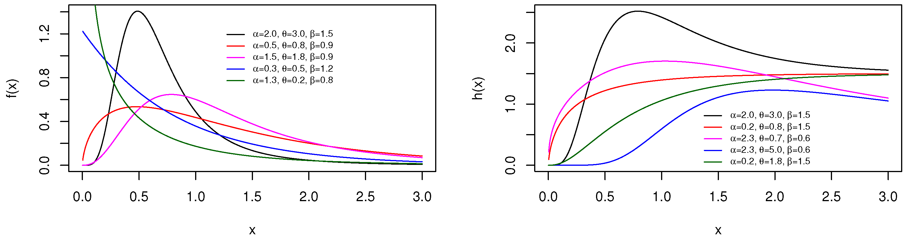
2.2.1. TBX Exponential Distribution
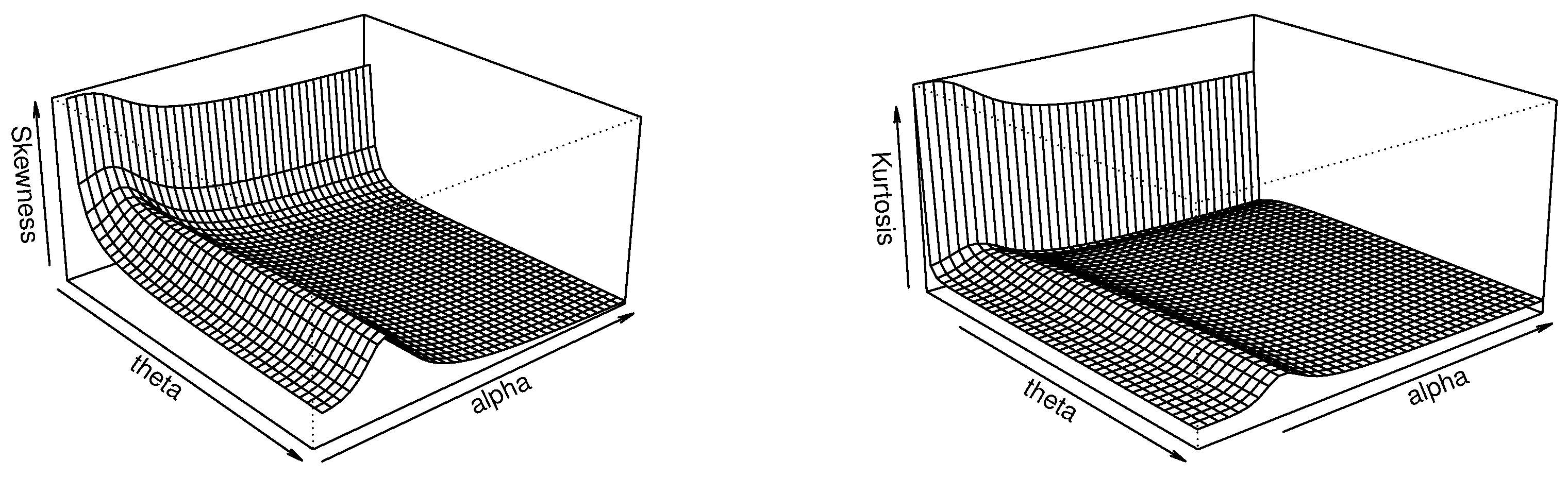
2.2.2. TBX Rayleigh Distribution
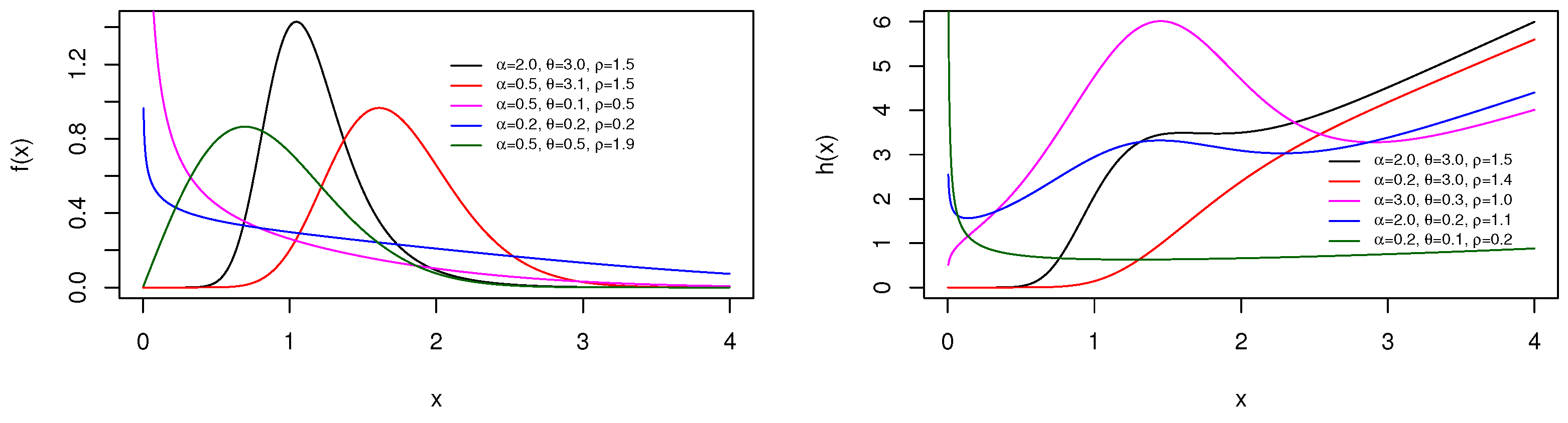
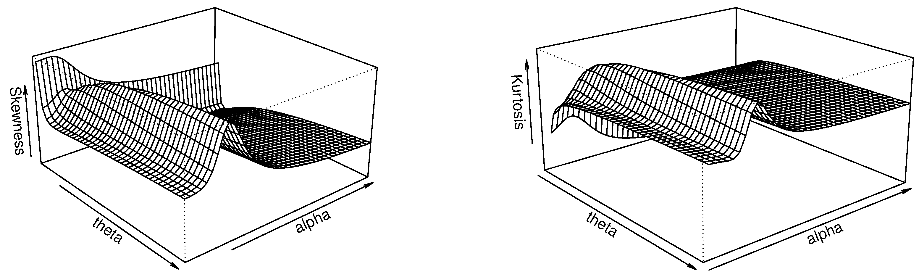
2.2.3. TBX Lindley Distribution
3. Mathematical Properties of the TBX-G Family
3.1. Asymptotic Study
3.2. First-Order Stochastic Dominance Study
3.3. Series Expansion Study
- TBXE distribution, for , we have:
- TBXR distribution, for , we have:
- TBXL distribution, for , we have:
3.4. Tsallis Entropy Study
3.5. Moment Study
3.6. Risk Measures
4. Statistical and Inferential Approaches
4.1. Methodology
4.2. Simulation
5. Applications to Actuarial and Financial Data
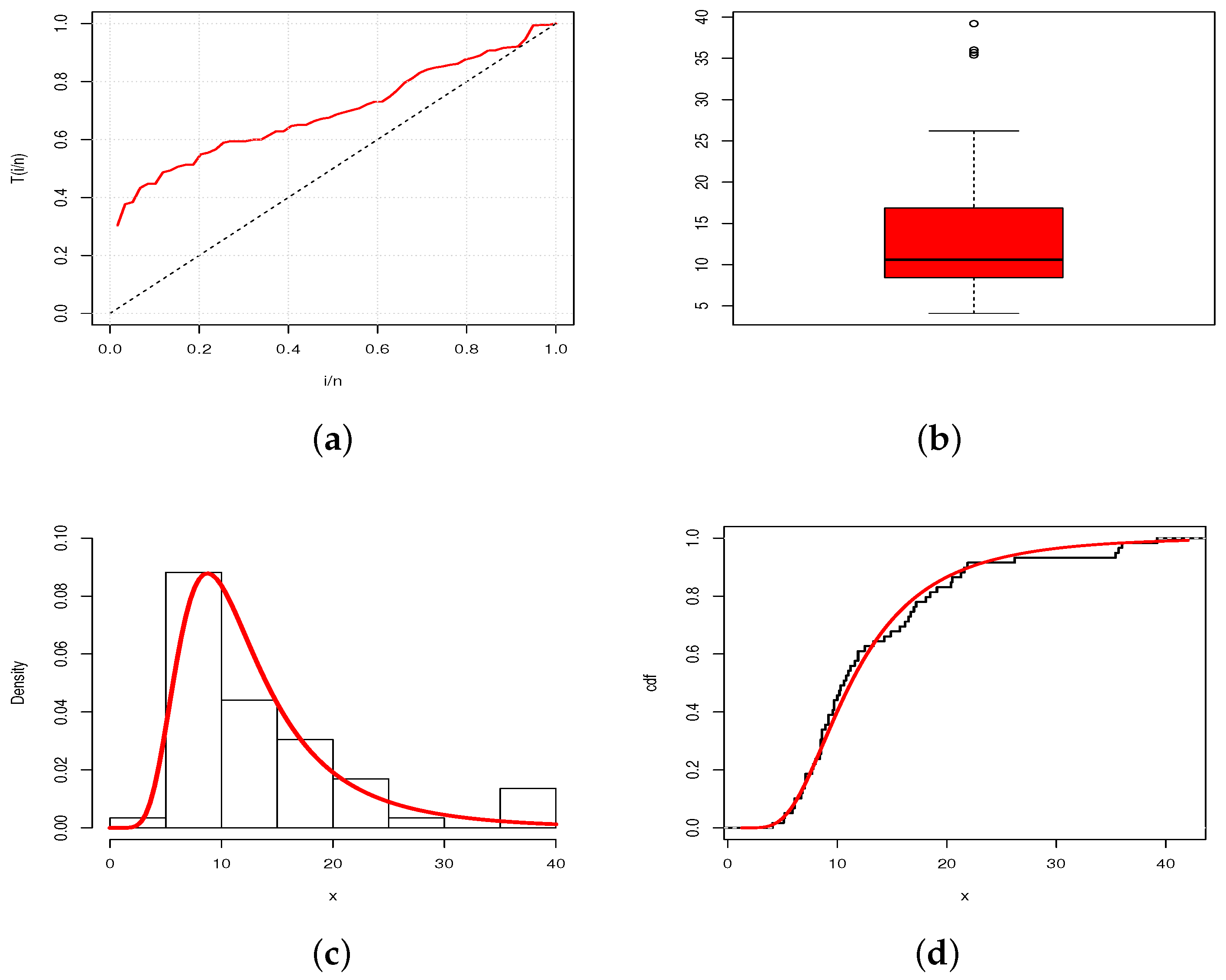
5.1. Data Fitting
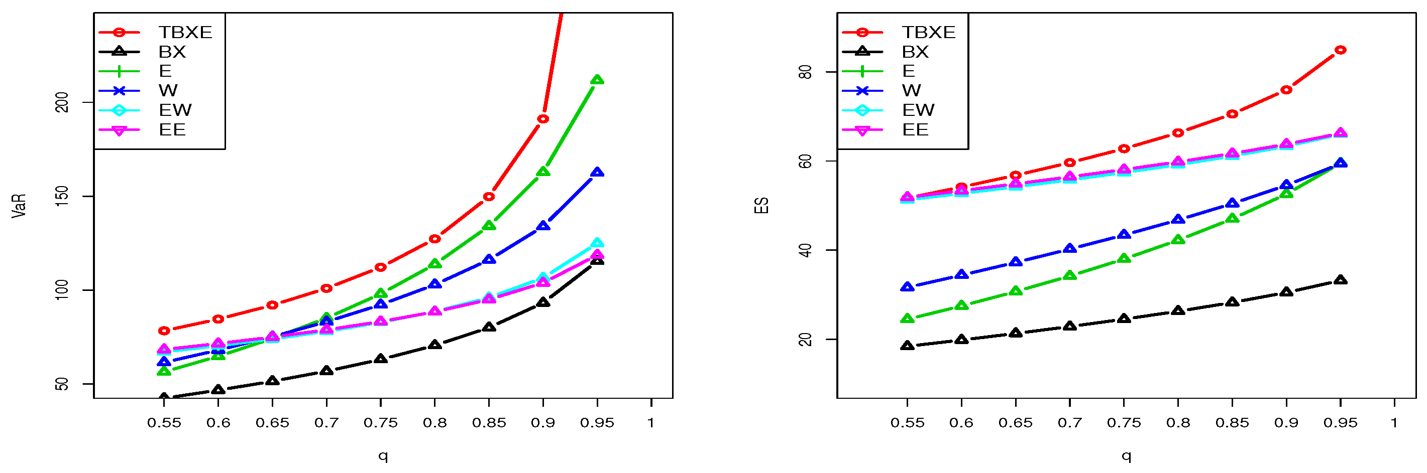
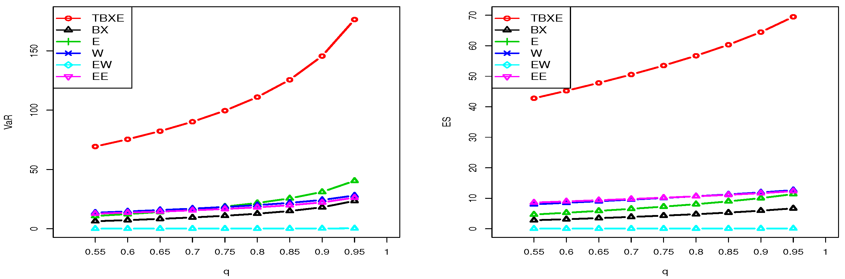
5.2. Estimation of and
6. Concluding Notes and Perspectives
6.1. Concluding Notes
6.2. Perspectives
Author Contributions
Funding
Institutional Review Board Statement
Informed Consent Statement
Data Availability Statement
Acknowledgments
Conflicts of Interest
References
- Brito, C.C.R.; Rêgo, L.C.; Oliveira, W.R.; Gomes-Silva, F. Method for generating distributions and families of probability distributions: The univariate case. Hacet. J. Math. Stat. 2019, 48, 897–930. [Google Scholar]
- Cordeiro, G.M.; Silva, R.B.; Nascimento, A.D.C. Recent Advances in Lifetime and Reliability Models; Bentham Sciences Publishers: Sharjah, United Arab Emirates, 2020. [Google Scholar]
- Tahir, M.H.; Cordeiro, G.G. Compounding of distributions: A survey and new generalized classes. J. Stat. Distrib. Appl. 2016, 3, 1–35. [Google Scholar] [CrossRef] [Green Version]
- Abid, A.H.; Abdulrazak, R.K. [0,1] truncated Fréchet-G generator of distributions. Appl. Math. 2017, 7, 51–66. [Google Scholar]
- Najarzadegan, H.; Alamatsaz, M.H.; Hayati, S. Truncated Weibull-G more flexible and more reliable than geta-G distribution. Int. J. Stat. Probab. 2017, 6, 1–17. [Google Scholar] [CrossRef] [Green Version]
- Bantan, R.A.; Jamal, F.; Chesneau, C.; Elgarhy, M. Truncated inverted Kumaraswamy generated family of distributions with applications. Entropy 2019, 21, 1089. [Google Scholar] [CrossRef] [Green Version]
- Aldahlan, M.A. Type II Fréchet generated family of distributions. Int. J. Math. Its Appl. 2019, 7, 221–228. [Google Scholar]
- Al-Babtain, A.A.; Elbatal, I.; Chesneau, C.; Jamal, F. The transmuted Muth generated class of distributions with applications. Symmetry 2020, 12, 1677. [Google Scholar] [CrossRef]
- Al-Babtain, A.A.; Elbatal, I.; Chesneau, C.; Jamal, F. Box-Cox gamma-G family of distributions: Theory and applications. Mathematics 2020, 8, 1801. [Google Scholar] [CrossRef]
- Al-Marzouki, S.; Jamal, F.; Chesneau, C.; Elgarhy, M. Topp-Leone odd Fréchet generated family of distributions with applications to Covid-19 datasets. CMES-Comput. Modeling Eng. Sci. 2020, 125, 437–458. [Google Scholar]
- Aldahlan, M.A.; Jamal, F.; Chesneau, C.; Elbatal, I.; Elgarhy, M. Exponentiated power generalized Weibull power series family of distributions: Properties. estimation and applications. PLoS ONE 2020, 15, e0230004. [Google Scholar] [CrossRef] [Green Version]
- Cordeiro, G.M.; Altun, E.; Korkmaz, M.C.; Pescim, R.R.; Afify, A.Z.; Yousof, H.M. The xgamma family: Censored regression modelling and applications. REVSTAT-Stat. J. 2020, 18, 593–612. [Google Scholar]
- Aldahlan, M.A.; Jamal, F.; Chesneau, C.; Elgarhy, M.; Elbatal, I. The truncated Cauchy power family of distributions with inference and applications. Entropy 2020, 22, 346. [Google Scholar] [CrossRef] [Green Version]
- Almarashi, A.M.; Elgarhy, M.; Jamal, F.; Chesneau, C. The exponentiated truncated inverse Weibull generated family of distributions with applications. Symmetry 2020, 12, 650. [Google Scholar] [CrossRef] [Green Version]
- Badr, M.A.; Elbatal, I.; Jamal, F.; Chesneau, C.; Elgarhy, M. The transmuted odd Fréchet-G family of distributions: Theory and applications. Mathematics 2020, 8, 958. [Google Scholar] [CrossRef]
- Yousof, H.M.; Rasekhi, M.; Alizadeh, M.; Hamedani, G.G. The Marshall-Olkin exponentiated generalized G family of distributions: Properties, applications and characterizations. J. Nonlinear Sci. Appl. 2020, 13, 34–52. [Google Scholar] [CrossRef]
- Bantan, R.A.R.; Chesneau, C.; Jamal, F.; Elgarhy, M. On the analysis of new Covid-19 cases in Pakistan using an exponentiated version of the M family of distributions. Mathematics 2020, 8, 953. [Google Scholar] [CrossRef]
- Bantan, R.A.R.; Jamal, F.; Chesneau, C.; Elgarhy, M. Type II Power Topp-Leone generated family of distributions with statistical inference and applications. Symmetry 2020, 12, 75. [Google Scholar] [CrossRef] [Green Version]
- Aslam, M.; Asghar, Z.; Hussain, Z.; Shah, S.F. A modified T-X family of distributions: Classical and Bayesian analysis. J. Taibah Univ. Sci. 2020, 14, 254–264. [Google Scholar] [CrossRef] [Green Version]
- Chesneau, C.; El Achi, T. Modified odd Weibull family of distributions: Properties and applications. J. Indian Soc. Probab. Stat. 2020, 21, 259–286. [Google Scholar] [CrossRef] [Green Version]
- Jamal, F.; Bakouch, H.S.; Nasir, M.A. A truncated general-G class of distributions with application to truncated Burr-G family. Revstat.- Stat. J. 2020, in press. [Google Scholar]
- Jamal, F.; Chesneau, C.; Elgarhy, M. Type II general inverse exponential family of distributions. J. Stat. Manag. Syst. 2020, 23, 617–641. [Google Scholar] [CrossRef] [Green Version]
- Nasir, M.A.; Tahir, M.H.; Chesneau, C.; Jamal, F.; Shah, M.A.A. The odd generalized gamma-G family of distributions: Properties, regressions and applications. Statistica 2020, 80, 3–38. [Google Scholar]
- ZeinEldin, R.A.; Chesneau, C.; Jamal, F.; Elgarhy, M.; Almarashi, A.M.; Al-Marzouki, S. Generalized truncated Fréchet generated family distributions and their applications. CMES-Comput. Modeling Eng. Sci. 2021, 126, 791–819. [Google Scholar] [CrossRef]
- Burr, I.W. Cumulative frequency functions. Ann. Math. Stat. 1942, 13, 215–232. [Google Scholar] [CrossRef]
- Ahmad, K.; Fakhry, M.; Jaheen, Z. Empirical Bayes estimation of P(Y<X) and characterizations of Burr-type X model. J. Stat. Plan. Inference 1997, 64, 297–308. [Google Scholar]
- Ahmad Sartawi, H.; Abu-Salih, M.S. Bayesian prediction bounds for the Burr type X model. Commun. Stat.-Theory Methods 1991, 20, 2307–2330. [Google Scholar] [CrossRef]
- Lio, Y.; Tsai, T.-R.; Aslam, M.; Jiang, N. Control charts for monitoring Burr type-X percentiles. Commun. Stat.-Simul. Comput. 2014, 43, 761–776. [Google Scholar] [CrossRef]
- Raqab, M.Z. Order statistics from the Burr type X model. Comput. Math. Appl. 1998, 36, 111–120. [Google Scholar] [CrossRef] [Green Version]
- Raqab, M.Z.; Kundu, D. Burr type X distribution: Revisited. J. Probab. Stat. Sci. 2006, 4, 179–193. [Google Scholar]
- Smith, J.B.; Wong, A.; Zhou, X. Higher order inference for stress-strength reliability with independent Burr-type X distributions. J. Stat. Comput. Simul. 2015, 85, 3092–3107. [Google Scholar] [CrossRef]
- Surles, J.G.; Padgett, W.J. Inference for P(Y<X) in the Burr type X model. Commun. Stat.-Theory Methods 1998, 7, 225–238. [Google Scholar]
- Surles, J.G.; Padgett, W.J. Inference for reliability and stress-strength for a scaled Burr Type X distribution. Lifetime Data Anal. 2001, 7, 187–200. [Google Scholar] [CrossRef] [PubMed]
- Surles, J.G.; Padgett, W.J. Some properties of a scaled Burr type X distribution. J. Stat. Plan. Inference 2005, 128, 271–280. [Google Scholar] [CrossRef]
- Yousof, H.M.; Afify, A.Z.; Hamedani, G.G.; Aryal, G. The Burr X generator of distributions for lifetime data. J. Stat. Theory Appl. 2016, 16, 288–305. [Google Scholar] [CrossRef] [Green Version]
- Korkmaz, M.C.; Altun, E.; Yousof, H.M.; Afify, A.Z.; Nadarajah, S. The Burr X Pareto distribution: Properties, applications and VaR estimation. J. Risk Financ. Manag. 2018, 11, 1. [Google Scholar] [CrossRef] [Green Version]
- Aarset, M.V. How to identify bathtub hazard rate. IEEE Trans. Reliab. 1987, 36, 106–108. [Google Scholar] [CrossRef]
- Gilchrist, W. Statistical Modelling with Quantile Functions; CRC Press: Abingdon, UK, 2000. [Google Scholar]
- Shaked, M.; Shanthikumar, J.G. Stochastic Orders; Wiley: New York, NY, USA, 2007. [Google Scholar]
- Amigo, J.M.; Balogh, S.G.; Hernandez, S. A brief review of generalized entropies. Entropy 2018, 20, 813. [Google Scholar] [CrossRef] [Green Version]
- Tsallis, C. Possible generalization of Boltzmann-Gibbs statistics. J. Stat. Phys. 1988, 52, 479–487. [Google Scholar] [CrossRef]
- Artzner, P.; Delbaen, F.; Eber, J.-M.; Heath, D. Coherent measures of risk. Math. Financ. 1999, 9, 203–228. [Google Scholar] [CrossRef]
- Fischer, M.; Moser, T.; Pfeuffer, M. A discussion on recent risk measures with application to credit risk: Calculating risk contributions and identifying risk concentrations. Risks 2018, 6, 142. [Google Scholar] [CrossRef] [Green Version]
- Casella, G.; Berger, R.L. Statistical Inference; Brooks/Cole Publishing Company: Bel Air, CA, USA, 1990. [Google Scholar]
- R Development Core Team. R: A Language and Environment for Statistical Computing; R Foundation for Statistical Computing: Vienna, Austria, 2005; ISBN 3-900051-07-0. Available online: http://www.R-project.org (accessed on 14 April 2021).
- Mead, M.E. A new generalization of Burr XII distribution. J. Stat. Adv. Theory Appl. 2014, 12, 53–71. [Google Scholar]
- Chan, S.; Nadarajah, S. Risk: An R package for financial risk measures. Comput. Econ. 2019, 53, 1337–1351. [Google Scholar] [CrossRef] [Green Version]
- Gijbels, I.; Omelka, M.; Pešta, M.; Veraverbeke, N. Score tests for covariate effects in conditional copulas. J. Multivar. Anal. 2017, 159, 111–133. [Google Scholar] [CrossRef]
- Maciak, M.; Okhrin, O.; Pešta, M. Infinitely stochastic micro reserving. Insur. Math. Econ. 2021, 100, 30–58. [Google Scholar] [CrossRef]
- Pešta, M.; Okhrin, O. Conditional least squares and copulae in claims reserving for a single line of business. Insur. Math. Econ. 2014, 56, 28–37. [Google Scholar] [CrossRef] [Green Version]
- Sherbakov, S. Modeling of the damaged state by the finite-element method on simultaneous action of contact and noncontact loads. J. Eng. Phys. Thermophys. 2012, 85, 472–477. [Google Scholar] [CrossRef]
- Sherbakov, S. Spatial stress-strain state of tribofatigue system in roll-shaft contact zone. Strength Mater. 2013, 45. [Google Scholar] [CrossRef]
- Sherbakov, S. Measurement and Real Time Analysis of Local Damage in Wear-and-Fatigue Tests. Devices Methods Meas. 2019, 10, 207–214. [Google Scholar] [CrossRef] [Green Version]


| Sample Size | Actual Values | AE | RMSE | ||||||
|---|---|---|---|---|---|---|---|---|---|
| 30 | 0.3 | 0.7 | 1.2 | 0.5537 | 0.8124 | 1.1760 | 0.6695 | 0.2679 | 0.3346 |
| 80 | 0.5279 | 0.7408 | 1.1247 | 0.6429 | 0.1302 | 0.2472 | |||
| 130 | 0.4911 | 0.7296 | 1.1310 | 0.6031 | 0.0989 | 0.2173 | |||
| 180 | 0.4759 | 0.7232 | 1.1310 | 0.5765 | 0.0818 | 0.1976 | |||
| 230 | 0.4587 | 0.7161 | 1.1448 | 0.5442 | 0.0721 | 0.1795 | |||
| 280 | 0.4276 | 0.7161 | 1.1448 | 0.5144 | 0.0642 | 0.1662 | |||
| 30 | 1.3 | 2.7 | 0.6 | 1.0669 | 3.4192 | 0.6530 | 0.7543 | 4.7441 | 0.1966 |
| 80 | 1.1540 | 2.7689 | 0.6120 | 0.6604 | 0.8594 | 0.1576 | |||
| 130 | 1.1975 | 2.6818 | 0.6018 | 0.5846 | 0.6084 | 0.1398 | |||
| 180 | 1.2315 | 2.6669 | 0.5973 | 0.5241 | 0.5153 | 0.1284 | |||
| 230 | 1.2481 | 2.6672 | 0.5971 | 0.4783 | 0.4576 | 0.1203 | |||
| 280 | 1.2640 | 2.6628 | 0.5944 | 0.4472 | 0.4174 | 0.1134 | |||
| 30 | 0.8 | 0.8 | 0.9 | 0.6695 | 0.9178 | 0.9476 | 0.6962 | 0.3263 | 0.2809 |
| 80 | 0.7074 | 0.8290 | 0.8894 | 0.6706 | 0.1497 | 0.2144 | |||
| 130 | 0.7187 | 0.8125 | 0.8125 | 0.6477 | 0.1135 | 0.1934 | |||
| 180 | 0.7339 | 0.8066 | 0.8760 | 0.6190 | 0.0952 | 0.1819 | |||
| 230 | 0.7268 | 0.8042 | 0.8802 | 0.5901 | 0.0846 | 0.1694 | |||
| 280 | 0.7380 | 0.8020 | 0.8779 | 0.5683 | 0.0761 | 0.1610 | |||
| 30 | 1.5 | 0.9 | 0.9 | 0.9432 | 1.0338 | 1.2239 | 0.7431 | 0.3945 | 0.4349 |
| 80 | 1.1262 | 0.9287 | 1.0851 | 0.6901 | 0.1767 | 0.3340 | |||
| 130 | 1.2224 | 0.9121 | 1.0370 | 0.6314 | 0.1347 | 0.3021 | |||
| 180 | 1.2828 | 0.9060 | 1.0103 | 0.5801 | 0.1152 | 0.2839 | |||
| 230 | 1.3237 | 0.8999 | 0.9885 | 0.5365 | 0.1001 | 0.2634 | |||
| 280 | 1.3556 | 0.8984 | 0.9749 | 0.5114 | 0.0924 | 0.2560 | |||
| 30 | 1.2 | 0.8 | 0.6 | 0.7988 | 0.8992 | 0.7166 | 0.7192 | 0.3198 | 0.2379 |
| 80 | 0.9468 | 0.8176 | 0.6501 | 0.6862 | 0.1493 | 0.1816 | |||
| 130 | 1.0275 | 0.8052 | 0.6271 | 0.6413 | 0.1133 | 0.1653 | |||
| 180 | 1.0539 | 0.7964 | 0.6208 | 0.6045 | 0.0944 | 0.1535 | |||
| 230 | 1.0804 | 0.7953 | 0.6154 | 0.5765 | 0.0847 | 0.1478 | |||
| 280 | 1.0974 | 0.7944 | 0.6129 | 0.5420 | 0.0766 | 0.1401 | |||
| 30 | 1.0 | 1.0 | 0.8 | 0.7735 | 1.1469 | 0.8711 | 0.7156 | 0.4412 | 0.2654 |
| 80 | 0.8561 | 1.0253 | 0.8068 | 0.6855 | 0.1976 | 0.2076 | |||
| 130 | 0.8889 | 1.0075 | 0.7974 | 0.6465 | 0.1514 | 0.1881 | |||
| 180 | 0.9068 | 1.0008 | 0.7930 | 0.6066 | 0.1279 | 0.1739 | |||
| 230 | 0.9156 | 0.9984 | 0.7931 | 0.5716 | 0.1137 | 0.1634 | |||
| 280 | 0.9347 | 0.9945 | 0.7885 | 0.5448 | 0.1036 | 0.1553 | |||
| 30 | 1.2 | 0.8 | 0.9 | 0.8092 | 0.9033 | 1.0767 | 0.7121 | 0.3203 | 0.3530 |
| 80 | 0.9476 | 0.8189 | 0.9739 | 0.6910 | 0.1504 | 0.2734 | |||
| 130 | 1.0226 | 0.8027 | 0.9405 | 0.6481 | 0.1143 | 0.2457 | |||
| 180 | 1.0763 | 0.7996 | 0.9251 | 0.6020 | 0.0951 | 0.2319 | |||
| 230 | 1.0842 | 0.7964 | 0.9221 | 0.5752 | 0.0844 | 0.2212 | |||
| 280 | 1.1167 | 0.7933 | 0.9107 | 0.5486 | 0.0764 | 0.2123 | |||
| 30 | 0.5 | 1.8 | 1.5 | 0.9069 | 2.3930 | 1.4504 | 0.7638 | 1.4810 | 0.3880 |
| 80 | 0.6344 | 2.0147 | 1.4201 | 0.7482 | 0.5264 | 0.2887 | |||
| 130 | 0.5924 | 1.9439 | 1.4294 | 0.6190 | 0.3896 | 0.2482 | |||
| 180 | 0.5499 | 1.9137 | 1.4450 | 0.5578 | 0.3264 | 0.2088 | |||
| 230 | 0.5349 | 1.8937 | 1.4489 | 0.5239 | 0.2821 | 0.1848 | |||
| 280 | 0.5096 | 1.8782 | 1.4604 | 0.4914 | 0.2556 | 0.1630 | |||
| Model | Parameters | MLEs (D1) | SEs (D1) | MLEs (D2) | SEs (D2) |
|---|---|---|---|---|---|
| TBXE | 2.6510 | 0.282 | 1.8533 | 0.3379 | |
| 10.4527 | 4.99 | 5.1464 | 2.0897 | ||
| 0.0152 | 0.0040 | 0.1191 | 0.0356 | ||
| BX | 0.0200 | 0.0012 | 0.0644 | 0.0056 | |
| 1.9912 | 0.4252 | 1.0310 | 0.1844 | ||
| EE | 0.05 | 0.006 | 0.1786 | 0.0232 | |
| 16.08 | 5.251 | 5.5321 | 1.4350 | ||
| E | 0.0142 | 0.0020 | 0.0741 | 0.0096 | |
| MOE | 0.0664 | 0.0082 | 0.2092 | 0.0308 | |
| a | 72.1333 | 41.0232 | 11.5647 | 5.2019 | |
| EW | 0.4333 | 0.4872 | 1.5481 | 0.9126 | |
| 0.6043 | 0.1992 | 0.4706 | 0.1308 | ||
| a | 130.3842 | 219.0512 | 88.6904 | 8.4074 | |
| OWE | 0.0028 | 0.0005 | 0.0164 | 0.0185 | |
| a | 14.2800 | 7.2812 | 6.6161 | 5.4439 | |
| b | 1.9155 | 0.1843 | 1.5472 | 1.5625 | |
| W | 0.0029 | 0.0006 | 0.0069 | 0.0028 | |
| 1.3611 | 0.0552 | 1.8215 | 0.1339 | ||
| TLE | 0.0242 | 0.0028 | 0.0893 | 0.0116 | |
| a | 15.9758 | 5.1955 | 5.5322 | 1.4347 |
| Model | AIC | CAIC | BIC | HQIC | A | W | K.S | p-Value | |
|---|---|---|---|---|---|---|---|---|---|
| TBXE | 265.329 | 536.658 | 537.102 | 542.839 | 539.066 | 0.716 | 0.125 | 0.111 | 0.471 |
| BX | 275.364 | 554.728 | 554.947 | 558.849 | 556.334 | 2.416 | 0.444 | 0.182 | 0.044 |
| EE | 267.487 | 538.973 | 539.191 | 543.094 | 540.578 | 1.090 | 0.201 | 0.113 | 0.447 |
| E | 304.967 | 611.934 | 612.006 | 613.995 | 612.737 | 1.755 | 0.324 | 0.387 | 0.00001 |
| MOE | 274.318 | 552.636 | 552.854 | 556.757 | 554.241 | 2.218 | 0.400 | 0.140 | 0.204 |
| EW | 266.190 | 538.379 | 538.824 | 544.561 | 540.787 | 0.896 | 0.163 | 0.117 | 0.408 |
| OWE | 281.963 | 569.927 | 570.371 | 576.108 | 572.334 | 3.312 | 0.608 | 0.187 | 0.034 |
| W | 291.235 | 586.470 | 586.688 | 590.591 | 588.075 | 2.065 | 0.380 | 0.332 | 0.00001 |
| TLE | 267.487 | 538.973 | 539.191 | 543.094 | 540.578 | 1.091 | 0.202 | 0.113 | 0.445 |
| Model | AIC | CAIC | BIC | HQIC | A | W | K.S | p-Value | |
|---|---|---|---|---|---|---|---|---|---|
| TBXE | 265.3401 | 383.0907 | 383.5271 | 389.3233 | 385.5237 | 0.3621 | 0.0623 | 0.0703 | 0.9321 |
| BX | 275.3641 | 399.3927 | 399.6070 | 403.5478 | 401.0147 | 1.9904 | 0.3112 | 0.1763 | 0.0509 |
| EE | 267.4865 | 386.4471 | 386.6614 | 390.6021 | 388.0690 | 0.8708 | 0.1442 | 0.1148 | 0.4180 |
| E | 304.9673 | 611.9345 | 612.0060 | 613.9950 | 612.7371 | 1.7555 | 0.3236 | 0.3869 | 0.0000 |
| MOE | 274.3689 | 552.7378 | 552.9560 | 556.8587 | 554.3430 | 2.2232 | 0.4015 | 0.1498 | 0.1481 |
| EW | 266.2673 | 538.5346 | 538.9790 | 544.7159 | 540.9423 | 0.9065 | 0.1651 | 0.1148 | 0.4282 |
| OWE | 199.4381 | 404.8762 | 405.3125 | 411.1088 | 407.3091 | 2.1691 | 0.3368 | 0.1446 | 0.1694 |
| W | 197.2967 | 398.5934 | 398.8077 | 402.7485 | 400.2154 | 1.8483 | 0.2897 | 0.1392 | 0.2025 |
| TLE | 191.2235 | 386.4471 | 386.6614 | 390.6021 | 388.0690 | 0.8708 | 0.1442 | 0.1148 | 0.4183 |
| q | TBXE | BX | EE | EW | W | E |
|---|---|---|---|---|---|---|
| 0.55 | 78.32 | 42.40 | 68.33 | 67.06 | 61.48 | 56.43 |
| 0.60 | 84.53 | 46.69 | 71.52 | 70.33 | 68.02 | 64.76 |
| 0.65 | 91.98 | 51.44 | 74.99 | 73.95 | 75.17 | 74.20 |
| 0.70 | 100.92 | 56.81 | 78.84 | 78.04 | 83.13 | 85.09 |
| 0.75 | 112.17 | 63.03 | 83.23 | 82.80 | 92.21 | 97.98 |
| 0.80 | 127.27 | 70.52 | 88.43 | 88.57 | 102.89 | 113.75 |
| 0.85 | 149.78 | 80.02 | 94.94 | 95.99 | 116.11 | 134.08 |
| 0.90 | 191.17 | 93.20 | 103.85 | 106.51 | 133.86 | 162.74 |
| 0.95 | 357.62 | 115.42 | 118.67 | 124.94 | 162.42 | 211.72 |
| q | TBXE | BX | EE | EW | W | E |
|---|---|---|---|---|---|---|
| 0.55 | 51.68 | 18.44 | 51.84 | 51.27 | 31.64 | 24.50 |
| 0.60 | 54.16 | 19.86 | 53.34 | 52.72 | 34.40 | 27.50 |
| 0.65 | 56.79 | 21.33 | 54.87 | 54.21 | 37.26 | 30.72 |
| 0.70 | 59.63 | 22.88 | 56.45 | 55.77 | 40.24 | 34.21 |
| 0.75 | 62.76 | 24.53 | 58.08 | 57.41 | 43.40 | 38.02 |
| 0.80 | 66.31 | 26.31 | 59.81 | 59.17 | 46.77 | 42.24 |
| 0.85 | 70.53 | 28.27 | 61.68 | 61.10 | 50.45 | 47.01 |
| 0.90 | 75.96 | 30.51 | 63.76 | 63.31 | 54.56 | 52.59 |
| 0.95 | 84.91 | 33.21 | 66.21 | 66.01 | 59.41 | 59.53 |
| q | TBXE | BX | EE | EW | W | E |
|---|---|---|---|---|---|---|
| 0.55 | 69.34 | 6.37 | 12.76 | 0.10 | 13.58 | 10.78 |
| 0.60 | 75.44 | 7.30 | 13.60 | 0.12 | 14.64 | 12.37 |
| 0.65 | 82.31 | 8.34 | 14.51 | 0.13 | 15.78 | 14.17 |
| 0.70 | 90.22 | 9.55 | 15.53 | 0.15 | 17.01 | 16.25 |
| 0.75 | 99.57 | 10.97 | 16.70 | 0.18 | 18.38 | 18.71 |
| 0.80 | 110.98 | 12.71 | 18.09 | 0.20 | 19.95 | 21.72 |
| 0.85 | 125.59 | 14.95 | 19.83 | 0.24 | 21.83 | 25.60 |
| 0.90 | 145.60 | 18.10 | 22.23 | 0.28 | 24.28 | 31.07 |
| 0.95 | 176.39 | 23.49 | 26.23 | 0.35 | 28.06 | 40.43 |
| q | TBXE | BX | EE | EW | W | E |
|---|---|---|---|---|---|---|
| 0.55 | 42.77 | 2.80 | 8.59 | 0.04 | 8.01 | 4.68 |
| 0.60 | 45.23 | 3.14 | 8.98 | 0.05 | 8.51 | 5.25 |
| 0.65 | 47.82 | 3.50 | 9.37 | 0.05 | 9.03 | 5.87 |
| 0.70 | 50.56 | 3.88 | 9.77 | 0.06 | 9.55 | 6.53 |
| 0.75 | 53.50 | 4.31 | 10.19 | 0.07 | 10.10 | 7.26 |
| 0.80 | 56.73 | 4.78 | 10.64 | 0.07 | 10.66 | 8.07 |
| 0.85 | 60.33 | 5.31 | 11.13 | 0.08 | 11.26 | 8.98 |
| 0.90 | 64.48 | 5.92 | 11.67 | 0.09 | 11.91 | 10.04 |
| 0.95 | 69.49 | 6.69 | 12.32 | 0.10 | 12.65 | 11.37 |
Publisher’s Note: MDPI stays neutral with regard to jurisdictional claims in published maps and institutional affiliations. |
© 2021 by the authors. Licensee MDPI, Basel, Switzerland. This article is an open access article distributed under the terms and conditions of the Creative Commons Attribution (CC BY) license (https://creativecommons.org/licenses/by/4.0/).
Share and Cite
Bantan, R.A.R.; Chesneau, C.; Jamal, F.; Elbatal, I.; Elgarhy, M. The Truncated Burr X-G Family of Distributions: Properties and Applications to Actuarial and Financial Data. Entropy 2021, 23, 1088. https://0-doi-org.brum.beds.ac.uk/10.3390/e23081088
Bantan RAR, Chesneau C, Jamal F, Elbatal I, Elgarhy M. The Truncated Burr X-G Family of Distributions: Properties and Applications to Actuarial and Financial Data. Entropy. 2021; 23(8):1088. https://0-doi-org.brum.beds.ac.uk/10.3390/e23081088
Chicago/Turabian StyleBantan, Rashad A. R., Christophe Chesneau, Farrukh Jamal, Ibrahim Elbatal, and Mohammed Elgarhy. 2021. "The Truncated Burr X-G Family of Distributions: Properties and Applications to Actuarial and Financial Data" Entropy 23, no. 8: 1088. https://0-doi-org.brum.beds.ac.uk/10.3390/e23081088