An Information Theoretic Interpretation to Deep Neural Networks ^†

Abstract

With the unprecedented performance achieved by deep learning, it is commonly believed that deep neural networks (DNNs) attempt to extract informative features for learning tasks. To formalize this intuition, we apply the local information geometric analysis and establish an information-theoretic framework for feature selection, which demonstrates the information-theoretic optimality of DNN features. Moreover, we conduct a quantitative analysis to characterize the impact of network structure on the feature extraction process of DNNs. Our investigation naturally leads to a performance metric for evaluating the effectiveness of extracted features, called the H-score, which illustrates the connection between the practical training process of DNNs and the information-theoretic framework. Finally, we validate our theoretical results by experimental designs on synthesized data and the ImageNet dataset.

1. Introduction

Due to the striking performance of deep learning in various application fields, deep neural networks (DNNs) have gained great attention in modern computer science. While it is a common understanding that the features extracted from the hidden layers of DNN are “informative” for learning tasks, the mathematical meaning of informative features in DNN is generally not clear. From the practical perspective, DNN models have obtained unprecedented performance in varying tasks, such as image recognition [1], language processing [2,3], and games [4,5]. However, the understanding of the feature extraction behind these models is relatively lacking, which poses challenges for their application in security-sensitive tasks, such as the autonomous vehicle.

To address this problem, there have been numerous research efforts, including both experimental and theoretical studies [6]. The experimental studies usually focus on some empirical properties of the feature extracted by DNNs, by visualizing the feature [7] or testing its performance on specific training settings [8] or learning tasks [9]. Though such empirical methods have provided some intuitive interpretations, the performance can highly depend on the data and network architecture used. For example, while the feature visualization works well on convolutional neural networks, its application to other networks is typically less effective [10].

In contrast, theoretical studies focus on the analytical properties of the extracted feature or the learning process in DNNs. Due to the complicated structure of DNNs, existing studies were often restricted to the networks of specific structures, e.g., network with infinite width [11] or two-layer network [12,13], to characterize the theoretical behaviors. However, the interpretation of the optimal feature remains unclear, which limits their further applications. To obtain better interpretability, tools and measures from information theory [14] have recently been applied to connect DNNs with general information processing problems [15]. For instance, the information bottleneck [16,17] employs the mutual information as the metric to quantify the informativeness of features in DNN, and other information metrics, such as the Kullback–Leibler (KL) divergence [18] and Weissenstein distance [19], are also used in different problems. However, there is still a disconnection between these information metrics and the performance objectives of the inference tasks that DNNs want to solve [20]. Therefore, it is, in general, difficult to match the DNN learning with the optimization of a particular information metric.

This paper aims to provide an information-theoretic interpretation to the feature extraction process in DNNs, to bridge the gap between the practical deep learning implementations and information-theoretic characterizations. To this end, we first propose an information-theoretic feature selection framework, which establishes an information metric to measure the performance of each given feature in inference tasks. In addition, we demonstrate that the optimal features extracted by DNNs coincide with the solutions of the information-theoretic feature selection problem, which share the same performance metric. Therefore, our results give an explicit interpretation of the learning goal of the back-propagation (BackProp) and stochastic gradient descent (SGD) operations in deep learning [21], which also lead to a performance metric for evaluating the effectiveness of the extracted features. Finally, we validate our theoretic characterizations using numerical experiments on both synthesized data and the ImageNet [22] dataset for image classification.

2. Preliminaries and Methods

2.1. Methodological Background

The main method used in our development is local information geometry [23,24], which characterizes the local geometric properties of the probability distribution space. The local information geometric method is closely related to the conventional Hirschfeld–Gebelein–Rényi (HGR) maximal correlation [25,26,27] problem, which has attracted increasing interest in the information theory community [28,29,30,31,32,33], and has also been applied in data analysis [34] and privacy studies [35].

Specifically, we use the local information geometric method to construct and investigate an information-theoretic feature selection problem in Section 3.1, which leads to an information metric of features and also demonstrates an SVD (singular value decomposition) structure of the feature selection process. Following the same analysis framework, we characterize the optimal feature extracted by DNNs in Section 3.2, and demonstrate that the same SVD structure is shared by DNNs. Based on the established connection, we then propose an effectiveness measure for DNNs, with details presented in Section 3.3.

2.2. Notations

Throughout this paper, we use X, $\mathcal{X}$, $P_X$, and x to represent a discrete random variable, the range, the probability distribution, and the value of X. In addition, for any function $s\left(X\right)\in {\mathbb{R}}^k$ of X, we use ${\mu }_s$ to denote the mean of $s\left(X\right)$, and “$\tilde{}$” to denote the centered variable with mean subtracted, e.g., $\tilde{s}\left(X\right)\triangleq s\left(X\right)-{\mu }_s$. Moreover, we use $\parallel ·\parallel$ and ${\parallel ·\parallel }_{\mathrm{F}}$ to denote the ${\ell }_2$-norm and the Frobenius norm, respectively. All logarithms in our analyses are base e, i.e., natural.

2.3. Local Information Geometry

The following concepts from local information geometry would be useful in our development.

Definition 1

($ϵ$-Neighborhood). Let ${\mathcal{P}}^{\mathcal{X}}$ denote the space of distributions on some finite alphabet $\mathcal{X}$, and let $relint\left({\mathcal{P}}^{\mathcal{X}}\right)$ denote the subset of strictly positive distributions. For a given $ϵ>0$, the ϵ-neighborhood of a distribution $P_X\in relint\left({\mathcal{P}}^{\mathcal{X}}\right)$ is defined by the ${\chi }^2$-divergence as

$${\mathcal{N}}_{ϵ}^{\mathcal{X}}\left(P_X\right)\triangleq \left\{P\in {\mathcal{P}}^{\mathcal{X}}:\sum _{x\in \mathcal{X}}\frac{{\left(P\left(x\right)-P_X\left(x\right)\right)}^2}{P_X\left(x\right)}\le {ϵ}^2\right\}.$$

Definition 2

($ϵ$-Dependence). The random variables $X,Y$ are called ϵ-dependent if $P_{XY}\in {\mathcal{N}}_{ϵ}^{\mathcal{X}\times \mathcal{Y}}\left(P_X{P}_Y\right)$.

Definition 3

($ϵ$-Attribute). A random variable U is called an ϵ-attribute of X if $P_{X|U}(·|u)\in {\mathcal{N}}_{ϵ}^{\mathcal{X}}\left(P_X\right)$, for all $u\in \mathcal{U}$.

We will focus on the small $ϵ$ regime, which we refer to as the local analysis regime. In addition, for any $P\in {\mathcal{P}}^{\mathcal{X}}$, we define the information vector$\varphi$ and feature function$L\left(x\right)$ corresponding to P, with respect to a reference distribution $P_X\in relint\left({\mathcal{P}}^{\mathcal{X}}\right)$, as

$$\varphi \left(x\right)\triangleq \frac{P\left(x\right)-P_X\left(x\right)}{\sqrt{P_X\left(x\right)}},L\left(x\right)\triangleq \frac{\varphi \left(x\right)}{\sqrt{P_X\left(x\right)}}.$$

(1)

This gives a three way correspondence $P\leftrightarrow \varphi \leftrightarrow L$ for all distributions in ${\mathcal{N}}_{ϵ}^{\mathcal{X}}\left(P_X\right)$, which will be useful in our derivations.

2.4. Modal Decomposition

Given a pair of discrete random variables $X,Y$ with the joint distribution $P_{XY}(x,y)$, the $\left|\mathcal{Y}\right|\times \left|\mathcal{X}\right|$ matrix $\tilde{\mathbf{B}}$ is defined as

$$\tilde{\mathbf{B}}(y,x)\triangleq \frac{P_{XY}(x,y)-P_X\left(x\right)P_Y\left(y\right)}{\sqrt{P_X\left(x\right)P_Y\left(y\right)}},$$

(2)

where $\tilde{\mathbf{B}}(y,x)$ is the $(y,x)$th entry of $\tilde{\mathbf{B}}$. The matrix $\tilde{\mathbf{B}}$ is referred to as the canonical dependence matrix (CDM) [24]. The SVD of $\tilde{\mathbf{B}}$ is referred to as the modal decomposition [24] of the joint distribution $P_{XY}$, which has the following property [18].

Lemma 1.

The SVD of $\tilde{\mathbf{B}}$ can be written as $\tilde{\mathbf{B}}={\sum }_{i=1}^K{\sigma }_i{\mathbf{\psi }}_i^Y{\left({\mathbf{\psi }}_i^X\right)}^{\mathrm{T}}$, where $K\triangleq min\left\{\right|\mathcal{X}|,|\mathcal{Y}\left|\right\}$, and ${\sigma }_i$ denotes the ith singular value with the ordering $1\ge {\sigma }_1\ge \dots \ge {\sigma }_K=0$, and ${\mathbf{\psi }}_i^Y$ and ${\mathbf{\psi }}_i^X$ are the corresponding left and right singular vectors with ${\psi }_K^X\left(x\right)=\sqrt{P_X\left(x\right)}$ and ${\psi }_K^Y\left(y\right)=\sqrt{P_Y\left(y\right)}$.

This SVD decomposes the feature spaces of $X,Y$ into maximally correlated features. To see that, consider the generalized canonical correlation analysis (CCA) problem:

$$\begin{array}{c}\hfill \underset{\begin{array}{c}\mathbb{E}\left[f_i\left(X\right)\right]=\mathbb{E}\left[g_i\left(Y\right)\right]=0\\ \mathbb{E}\left[f_i\left(X\right)f_j\left(X\right)\right]=\mathbb{E}\left[g_i\left(Y\right)g_j\left(Y\right)\right]={\delta }_{ij}\end{array}}{max}\sum _{i=1}^k\mathbb{E}\left[f_i\left(X\right)g_i\left(Y\right)\right],\end{array}$$

(3)

where ${\delta }_{ij}$ denotes the Kronecker delta function. It can be shown that for any $1\le k\le K-1$, the optimal features are $f_i\left(x\right)={\psi }_i^X\left(x\right)/\sqrt{P_X\left(x\right)}$, and $g_i\left(y\right)={\psi }_i^Y\left(y\right)/\sqrt{P_Y\left(y\right)}$, for $i=0,\dots ,K-1$, where ${\psi }_i^X\left(x\right)$ and ${\psi }_i^Y\left(y\right)$ are the xth and yth entries of ${\mathbf{\psi }}_i^X$ and ${\mathbf{\psi }}_i^Y$, respectively [18]. The special case $k=1$ corresponds to the HGR maximal correlation [25,26,27], and the optimal features can be computed from the ACE (Alternating Conditional Expectation) algorithm [36].

2.5. Deep Neural Networks

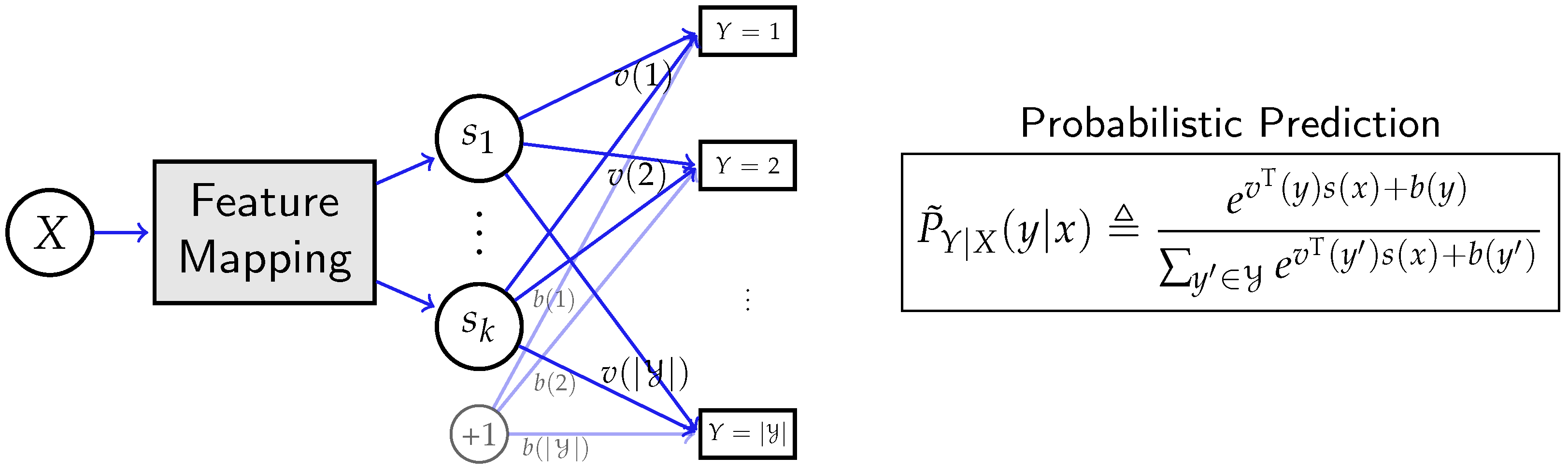
The architecture of deep neural networks (under log-loss) can be depicted as Figure 1, where X is the input data, e.g., images, audios, or natural languages. Moreover, Y is the objective to predict, which can represent a discrete label in classification tasks, or represent target natural languages in machine translations [37]. Specifically, for given data X, the network produces a (trainable) feature mapping to generate k-dimensional feature $s\left(x\right)={(s_1,\dots ,s_k)}^{\mathrm{T}}$. In practice, the feature mapping block (depicted as the gray block in Figure 1) is typically composed of hundreds and thousands of functional components (e.g., residual block [1]) with different types of layers, and may contain recurrent structure, e.g., LSTM (Long Short-Term Memory) [38]. In general, the internal structure of the feature mapping can have various different types of designs, depending on the learning tasks.

After obtaining the feature $s\left(X\right)$, the Y is then predicted by the probability distribution ${\tilde{P}}_{Y|X}^{(s,v,b)}$ of the form

$$\begin{array}{c}\hfill {\tilde{P}}_{Y|X}^{(s,v,b)}\left(y\right|x)\triangleq \frac{e^{v^{\mathrm{T}}\left(y\right)s\left(x\right)+b\left(y\right)}}{{\sum }_{y^{\prime }\in \mathcal{Y}}{e}^{v^{\mathrm{T}}\left(y^{\prime }\right)s\left(x\right)+b\left(y^{\prime }\right)}},\end{array}$$

(4)

which is obtained by applying the softmax function [39] on $v^{\mathrm{T}}\left(y\right)s\left(x\right)+b\left(y\right)$, where $v(·)$ and $b(·)$ are the weights and biases in the last layer, respectively (this is equivalent to the common practice that denotes weight and biases by the matrix ${[v\left(1\right),\dots ,v(\left|\mathcal{Y}\right|\left)\right]}^{\mathrm{T}}$ and the vector ${[b\left(1\right),\dots ,b(\left|\mathcal{Y}\right|\left)\right]}^{\mathrm{T}}$, respectively. However, as we will show later, expressing weights v and biases b as mappings of y can better illustrate their roles in feature selection). We will use ${\tilde{P}}_{Y|X}$ to refer to ${\tilde{P}}_{Y|X}^{(s,v,b)}$ when there is no ambiguity.

Then, for a given training set of labeled samples $(x_i,y_i)$, for $i=1,\dots ,N$, all the parameters in the network, including v, b, as well as those in the feature mapping block, are chosen to maximize the log-likelihood function (or, equivalently, minimize the log-loss)

$$\begin{array}{c}\hfill \frac{1}{N}\sum _{i=1}^{N}log{\tilde{P}}_{Y|X}\left(y_i\right|x_i).\end{array}$$

(5)

The procedure of choosing such parameters is called the training of network, which can be performed by stochastic gradient descent (SGD) or its variants [21]. With a trained network, the label $\widehat{y}$ for a new data sample x can be predicted by the maximum a posteriori (MAP) estimation, i.e., $\widehat{y} = {arg\; max}_{y\in \mathcal{Y}}{\tilde{P}}_{Y|X}\left(y\right|x).$ Specifically, when we make predictions for samples in a test dataset, the proportion of samples with correct prediction (i.e., $\widehat{y}=y$) over all samples is called the test accuracy.

3. Results

3.1. Information-Theoretic Feature Selection

Suppose that, given random variables $X,Y$ with joint distribution $P_{XY}$, we want to infer about an attribute V of Y from observed i.i.d. samples $x_1,\dots ,x_n$ of X. When the statistical model $P_{X|V}$ is known, the optimal decision rule is the log-likelihood ratio test, where the log-likelihood function can be viewed as the optimal feature for inference. However, in many practical situations [18], it is hard to identify the model of the targeted attribute, and it is necessary to select low-dimensional informative features of X for inference tasks before knowing the model. An information-theoretic formulation of such feature selection problem is the universal feature selection problem [24], which we formalize as follows.

To begin, for an attribute V, we refer to ${\mathcal{C}}_{\mathcal{Y}}=\left\{\mathcal{V},\{P_V\left(v\right),v\in \mathcal{V}\},\{{\mathbf{\varphi }}_v^{Y|V},v\in \mathcal{V}\}\right\},$ as the configuration of V, where ${\varphi }_v^{Y|V}\leftrightarrow P_{Y|V}(·|v)$ is the information vector specifying the corresponding conditional distribution $P_{Y|V}(·|v)$. The configuration of V models the statistical correlation between V and Y. In the sequel, we focus on the local analysis regime, for which we assume that all the attributes V of our interests to detect are $ϵ$-attributes of Y. As a result, the corresponding configuration satisfies $∥{\mathbf{\varphi }}_v^{Y|V}∥\le ϵ$, for all $v\in \mathcal{V}$. We refer to such configurations as ϵ-configurations. The configuration of V is unknown in advance but assumed to be generated from a rotational invariant ensemble (RIE).

Definition 4

(RIE). Two configurations ${\mathcal{C}}_{\mathcal{Y}}$ and ${\tilde{\mathcal{C}}}_{\mathcal{Y}}$ defined as

$${\mathcal{C}}_{\mathcal{Y}}\triangleq \left\{\mathcal{V},\{P_V\left(v\right),v\in \mathcal{V}\},\{{\mathbf{\varphi }}_v^{Y|V},v\in \mathcal{V}\}\right\},$$

$${\tilde{\mathcal{C}}}_{\mathcal{Y}}\triangleq \left\{\mathcal{V},\{P_V\left(v\right),v\in \mathcal{V}\},\{\tilde{\mathbf{\varphi }}{\phantom{\varphi }}_v^{Y|V},v\in \mathcal{V}\}\right\}$$

are called rotationally equivalent, if there exists a unitary matrix $\mathbf{Q}$ such that $\tilde{\mathbf{\varphi }}{\phantom{\varphi }}_v^{Y|V}=\mathbf{Q}{\mathbf{\varphi }}_v^{Y|V}$, for all $v\in \mathcal{V}$. Moreover, a probability measure defined on a set of configurations is called an RIE, if all rotationally equivalent configurations have the same measure.

The RIE can be interpreted as assigning a uniform measure to the attributes with the same level of distinguishability. To infer about the attribute V, we construct a k-dimensional feature vector $h^k=(h_1,\dots ,h_k)$, for some $1\le k\le K-1$, of the form

$$\begin{array}{c}\hfill h_i=\frac{1}{n}\sum _{l=1}^n{f}_i\left(x_l\right),i=1,\dots ,k,\end{array}$$

(6)

for some choices of feature functions $f_i$. Our goal is to determine the $f_i$ such that the optimal decision rule based on $h^k$ achieves the smallest possible error probability, where the performance is averaged over the possible ${\mathcal{C}}_{\mathcal{Y}}$ generated from an RIE. In turn, we denote ${\xi }_i^X\leftrightarrow f_i$ as the corresponding information vector, and define the matrix ${\mathrm{\Xi }}^X\triangleq [{\mathbf{\xi }}_1^X\dots {\mathbf{\xi }}_k^X]$.

Theorem 1

(Universal Feature Selection). For $v,v^{\prime }\in \mathcal{V}$, let $E_{h^k}(v,v^{\prime })$ be the error exponent associated with the pairwise error probability distinguishing v and $v^{\prime }$ based on $h^k$, then the expected error exponent over a given RIE defined on the set of ϵ-configurations is given by

$$\begin{array}{cc}\hfill \mathbb{E}\left[E_{h^k}(v,v^{\prime })\right]& =\frac{C_0}{2}·{∥\tilde{\mathbf{B}}{\mathrm{\Xi }}^X{\left({\left({\mathrm{\Xi }}^X\right)}^{\mathrm{T}}{\mathrm{\Xi }}^X\right)}^{-\frac{1}{2}}∥}_{\mathrm{F}}^2+o\left({ϵ}^2\right),\hfill \end{array}$$

(7)

where $C_0\triangleq \frac{1}{4\left|\mathcal{Y}\right|}·\mathbb{E}\left[{∥{\mathbf{\varphi }}_v^{Y|V}-{\mathbf{\varphi }}_{v^{\prime }}^{Y|V}∥}^2\right]$ is independent of the choices of $f_i$’s, and the expectations $\mathbb{E}\left[·\right]$ are taken over this RIE.

Proof. 

See Appendix A. □

As a result of (7), designing the ${\mathbf{\xi }}_i^X$ as the singular vectors ${\mathbf{\psi }}_i^X$ of $\tilde{\mathbf{B}}$, for $i=1,\dots ,k$, optimizes (7) for all RIEs, pairs of $(v,v^{\prime })$, and $ϵ$-configurations. Thus, the feature functions corresponding to ${\mathbf{\psi }}_i^X$ are universally optimal for inferring the unknown attribute V. Moreover, (7) naturally leads to an information metric ${∥\tilde{\mathbf{B}}{\mathrm{\Xi }}^X{\left({\left({\mathrm{\Xi }}^X\right)}^{\mathrm{T}}{\mathrm{\Xi }}^X\right)}^{-\frac{1}{2}}∥}_{\mathrm{F}}^2$ for any feature ${\mathrm{\Xi }}^X$ of X, measured by projecting the normalized ${\mathrm{\Xi }}^X$ through a linear projection $\tilde{\mathbf{B}}$. This information metric quantifies how informative a feature of X is when solving inference problems with respect to Y and is optimized when designing features by singular vectors of $\tilde{\mathbf{B}}$. Thus, we can interpret the universal feature selection as solving the most informative features for data inferences via the SVD of $\tilde{\mathbf{B}}$, which also coincides with the maximally correlated features in (3). Later, we will show that the feature selection in DNNs shares the same information metric as universal feature selection in the local analysis regime.

3.2. Feature Extraction in Deep Neural Networks

3.2.1. Network with Ideal Expressive Power

For convenience of analysis, we first consider the ideal case where the neural network can express any feature mapping $s(·)$ as desired. While this assumption can be rather strong, the existence of such ideal networks is guaranteed by the universal approximation theorem [40]. In addition, one goal of practical network designs is to approximate the ideal networks and obtain sufficient expressive power. For such networks, we will show that when $X,Y$ are $ϵ$-dependent, the extracted feature $s\left(x\right)$ and weights $v\left(y\right)$ coincide with the solutions of the universal feature selection.

To begin, we use $P_{XY}$ to denote the joint empirical distribution of the labeled samples $(x_i,y_i),i=1,\dots ,N$, and $P_X,P_Y$ to denote the corresponding marginal distributions. Then, the objective function of (5) is the empirical average of the log-likelihood function

$$\begin{array}{c}\hfill \frac{1}{N}\sum _{i=1}^{N}log{\tilde{P}}_{Y|X}\left(y_i\right|x_i)={\mathbb{E}}_{P_{XY}}\left[log{\tilde{P}}_{Y|X}\left(Y\right|X)\right].\end{array}$$

Therefore, maximizing this empirical average is equivalent as minimizing the KL divergence:

$$\begin{array}{c}\hfill (s^{*},v^{*},b^{*})=\underset{(s,v,b)}{arg\; min}D(P_{XY}\parallel P_X{\tilde{P}}_{Y|X}^{(s,v,b)}).\end{array}$$

(8)

This can be interpreted as finding the best fitting to empirical joint distribution $P_{XY}$ by distributions of the form $P_X{\tilde{P}}_{Y|X}^{(s,v,b)}$. In our development, it is more convenient to denote the bias by $d\left(y\right)=b\left(y\right)-log{P}_Y\left(y\right)$, for $y\in \mathcal{Y}$. Then, the following lemma illustrates the explicit constraint on the problem (8) in the local analysis regime.

Lemma 2.

If $X,Y$ are ϵ-dependent, then the optimal $v,d$ for (8) satisfy

$$\begin{array}{c}\hfill |{\tilde{v}}^{\mathrm{T}}\left(y\right)s\left(x\right)+\tilde{d}\left(y\right)|=O\left(ϵ\right),forallx\in \mathcal{X},y\in \mathcal{Y}.\end{array}$$

(9)

Proof. 

See Appendix B. □

In turn, we take (9) as the constraint for solving the problem (8) in the local analysis regime. Moreover, we define the information vectors for zero-mean vectors $\tilde{s}$, $\tilde{v}$ as ${\xi }^X\left(x\right)=\sqrt{P_X\left(x\right)}\tilde{s}\left(x\right)$, ${\xi }^Y\left(y\right)=\sqrt{P_Y\left(y\right)}\tilde{v}\left(y\right)$, and define matrices

$$\begin{array}{c}\hfill {\mathrm{\Xi }}^Y\triangleq {\left[\begin{array}{c}\begin{array}{ccc}{\xi }^Y\left(1\right)& \cdots & {\xi }^Y\left(\right|\mathcal{Y}\left|\right)\end{array}\end{array}\right]}^{\mathrm{T}},{\mathrm{\Xi }}^X\triangleq {\left[\begin{array}{ccc}{\xi }^X\left(1\right)& \cdots & {\xi }^X\left(\right|\mathcal{X}\left|\right)\end{array}\right]}^{\mathrm{T}}.\end{array}$$

Lemma 3.

The KL divergence (8) in the local analysis regime (9) can be expressed as

$$\begin{array}{cc}\hfill D(P_{XY}\parallel P_X{\tilde{P}}_{Y|X}^{(s,v,b)})& =\frac{1}{2}{∥\tilde{\mathbf{B}}-{\mathrm{\Xi }}^Y{\left({\mathrm{\Xi }}^X\right)}^{\mathrm{T}}∥}_{\mathrm{F}}^2+\frac{1}{2}{\eta }^{(v,b)}\left(s\right)+o\left({ϵ}^2\right),\hfill \end{array}$$

(10)

where ${\eta }^{(v,b)}\left(s\right)\triangleq {\mathbb{E}}_{P_Y}\left[{({\mu }_s^{\mathrm{T}}\tilde{v}\left(Y\right)+\tilde{d}\left(Y\right))}^2\right]$.

Proof. 

See Appendix C. □

Lemma 3 reveals key insights for feature selection in neural networks. To see this, we consider the following two learning problems: learning the optimal weight v for given s and learning the optimal feature s for given v.

For the case that s is fixed, we can optimize (10) with ${\mathrm{\Xi }}^X$ fixed and obtain the following optimal weights:

Theorem 2.

For fixed ${\mathrm{\Xi }}^X$ and ${\mu }_s$, the optimal ${\mathrm{\Xi }}^Y{}^{*}$ to minimize (10) is given by

$$\begin{array}{c}\hfill {\mathrm{\Xi }}^Y{}^{*}=\tilde{\mathbf{B}}{\mathrm{\Xi }}^X{\left({\left({\mathrm{\Xi }}^X\right)}^{\mathrm{T}}{\mathrm{\Xi }}^X\right)}^{-1},\end{array}$$

(11)

and the optimal weights ${\tilde{v}}^{*}$ and bias ${\tilde{d}}^{*}$ are

$$\begin{array}{c}\hfill {\tilde{v}}^{*}\left(y\right)={\mathbb{E}}_{P_{X|Y}}\left[{\mathrm{\Lambda }}_{\tilde{s}\left(X\right)}^{-1}\tilde{s}\left(X\right)|Y=y\right],{\tilde{d}}^{*}\left(y\right)=-{\mu }_s^{\mathrm{T}}\tilde{v}\left(Y\right).\end{array}$$

(12)

where ${\mathrm{\Lambda }}_{\tilde{s}\left(X\right)}$ denotes the covariance matrix of $\tilde{s}\left(X\right)$.

Proof. 

See Appendix D. □

Specifically, when $s\left(x\right)=x$, Theorem 2 gives the optimal weights for softmax regression. Note that Equation (11) can be viewed as a projection of the input feature $\tilde{s}\left(x\right)$, to a feature $v\left(y\right)$ computable from the value of y, which is the most correlated feature to $\tilde{s}\left(x\right)$. The solution is given by the operation that left multiplies $\tilde{\mathbf{B}}$ matrix, which we refer to as forward feature projection.

Remark 1.

While we assume the continuous input $s\left(x\right)$ is a function of a discrete variable X, we only need the labeled samples between s and Y to compute the weights and bias from the conditional expectation (12), and the correlation between X and s is irrelevant. Thus, our analysis for weights and bias can be applied to continuous input networks by just ignoring X and taking s as the real input to network.

We then consider the “backward feature projection” problem, which attempts to find informative feature $s^{*}\left(X\right)$ to minimize the loss (10) with given weights and bias. In particular, we can show that the solution of this backward feature projection is precisely symmetric to the forward one.

Theorem 3.

For fixed ${\mathrm{\Xi }}^Y$ and $\tilde{d}$, the optimal ${\mathrm{\Xi }}^X{}^{*}$ to minimize (10) is given by

$$\begin{array}{c}\hfill {\mathrm{\Xi }}^X{}^{*}={\tilde{\mathbf{B}}}^{\mathrm{T}}{\mathrm{\Xi }}^Y\left(\right({\mathrm{\Xi }}^Y{)}^{\mathrm{T}}{\mathrm{\Xi }}^Y{)}^{-1},\end{array}$$

(13)

and the optimal feature function $s^{*}$, which are decomposed to ${\tilde{s}}^{*}$ and ${\mu }_s^{*}$, is given by

$$\begin{array}{cc}\hfill {\tilde{s}}^{*}\left(x\right)& ={\mathbb{E}}_{P_{Y|X}}\left[{\mathrm{\Lambda }}_{\tilde{v}\left(Y\right)}^{-1}\tilde{v}\left(Y\right)|X=x\right],\hfill \\ \hfill {\mu }_s^{*}& =-{\mathrm{\Lambda }}_{\tilde{v}\left(Y\right)}^{-1}{\mathbb{E}}_{P_Y}\left[\tilde{v}\left(Y\right)\tilde{d}\left(Y\right)\right],\hfill \end{array}$$

(14)

where ${\mathrm{\Lambda }}_{\tilde{v}\left(Y\right)}$ denotes the covariance matrix of $\tilde{v}\left(Y\right)$.

Proof. 

See Appendix D. □

Finally, when both s and $(v,b)$ (and hence ${\mathrm{\Xi }}^X,{\mathrm{\Xi }}^Y,d$) can be designed, the optimal $({\mathrm{\Xi }}^Y,{\mathrm{\Xi }}^X)$ corresponds to the low rank factorization of $\tilde{\mathbf{B}}$, and the solutions coincide with the universal feature selection.

Theorem 4.

The optimal solutions for weights and bias to minimize (10) are given by $\tilde{d}\left(y\right)=-{\mu }_s^{\mathrm{T}}\tilde{v}\left(y\right)$, and ${({\mathrm{\Xi }}^Y,{\mathrm{\Xi }}^X)}^{*}$ chosen as the largest k left and right singular vectors of $\tilde{\mathbf{B}}$.

Proof. 

See Appendix E. □

Therefore, we conclude that the learning of neural networks, when both s and $(v,b)$ are designable, is to extract the most correlated aspects of the input data X and the label Y that are informative features for data inferences from universal feature selection.

In the practical learning process of DNN, the BackProp updates the weights of the softmax layer and those on the previous layer(s) in an iterative manner. As we have illustrated in Lemma 3, such iterative updates will converge to the same solution as the alternating between the forward feature projection (11) and the backward feature projection (13), which is indeed the power method to solve the SVD for $\tilde{\mathbf{B}}$ [41], also known as the Alternating Conditional Expectation (ACE) algorithm [36].

Remark 2.

From Theorem 4, for a neural network with sufficient expressive power, the trained feature depends only on the distribution of input data rather than the training process. It is worth mentioning that this result does not contradict the practice that trained weights in hidden layers can be different during each training run. In fact, due to the over-parameterized nature of practical network designs, there exist multiple choices of weights in hidden layers to express the same optimal feature $s\left(x\right)$.

3.2.2. Network with Restricted Expressive Power

The analysis of the previous section has considered neural networks with ideal expressive power, where the feature $s\left(X\right)$ can be selected as any desired function. In general, however, the form of feature functions that can be generalized is often limited by the network structure. In the following, we consider networks with restricted expressive power to characterize the impacts of network structure on the extracted feature.

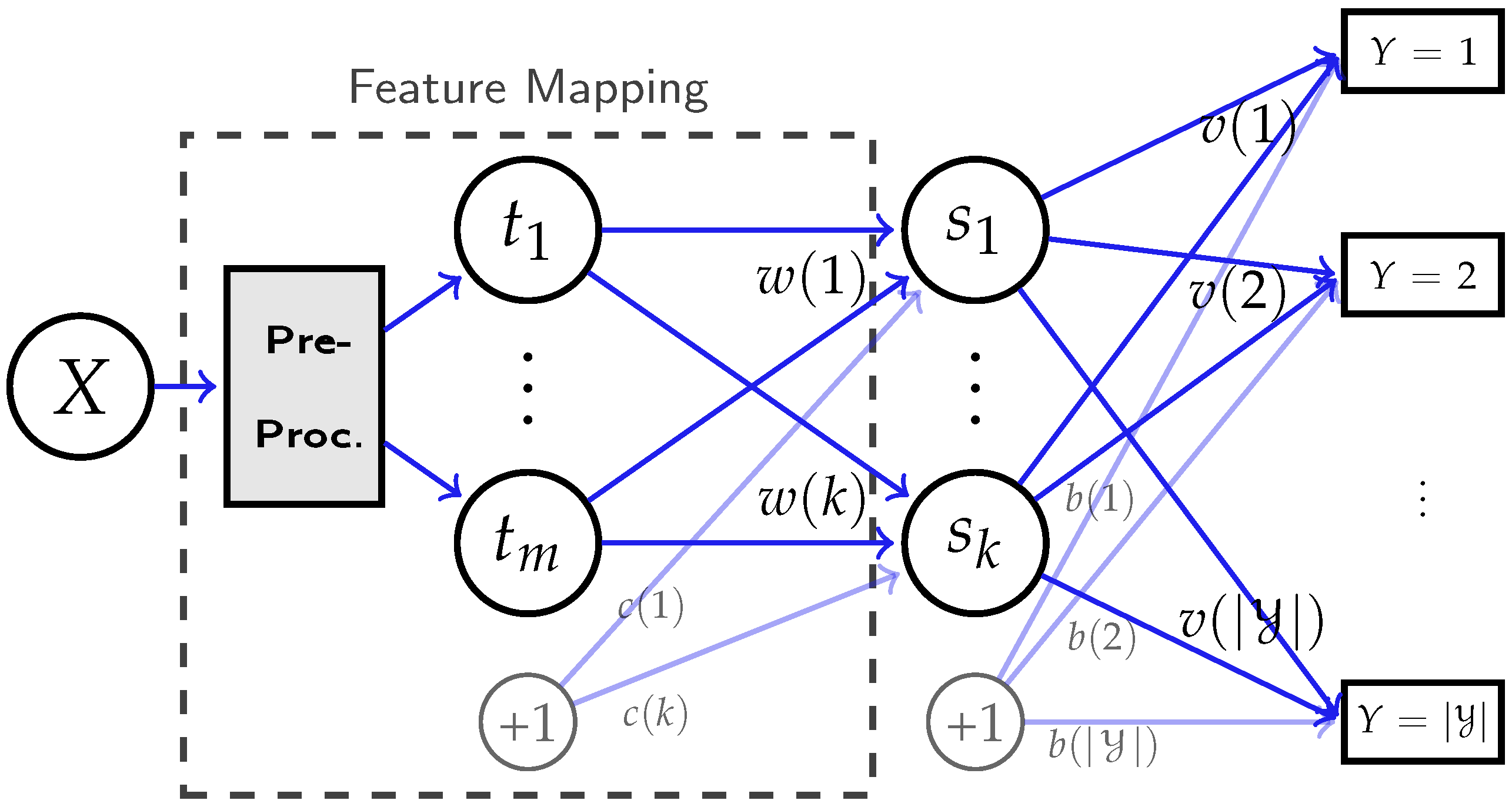
For illustration, we consider the neural network with a hidden layer of k nodes, and a zero-mean continuous input $t={[t_1\cdots t_m]}^{\mathrm{T}}\in {\mathbb{R}}^m$ to this hidden layer, where t is assumed to be a function $t\left(x\right)$ of some discrete variable X. Our goal is to analyze the weights and bias in this layer with labeled samples $(t\left(x_i\right),y_i)$. Assume the activation function of the hidden layer is a generally smooth function $\sigma (·)$, then the output $s_z\left(X\right)$ of the z-th hidden node is

$$\begin{array}{c}\hfill s_z\left(x\right)=\sigma \left(w^{\mathrm{T}}\left(z\right)t\left(x\right)+c\left(z\right)\right),\mathrm{for}z=1,\dots ,k,x\in \mathcal{X},\end{array}$$

(15)

where $w\left(z\right)\in {\mathbb{R}}^m$ and $c\left(z\right)\in \mathbb{R}$ are the weights and bias from input layer to hidden layer as shown in Figure 2. We denote $s={[s_1\cdots s_k]}^{\mathrm{T}}$ as the input vector to the output classification layer.

To interpret the feature selection in hidden layers, we fix $\left(v\right(y),b(y\left)\right)$ at the output layer and consider the problem of designing $\left(w\right(z),c(z\left)\right)$ to minimize the loss function (8) at the output layer. Ideally, we should have picked $w\left(z\right)$ and $c\left(z\right)$ to generate $s\left(x\right)$ to match $s^{*}\left(x\right)$ from (14), which minimizes the loss. However, here we have the constraint that $s\left(x\right)$ must take the form of (15) and, intuitively, the network should select $w\left(z\right),c\left(z\right)$ so that $s\left(x\right)$ is close to $s^{*}\left(x\right)$. Our goal is to quantify the notion of such closeness.

To develop insights on feature selection in hidden layers, we again focus on the local analysis regime, where the weights and bias are assumed to satisfy the local constraint

$$\begin{array}{c}\hfill \left|{\tilde{v}}^{\mathrm{T}}\left(y\right)s\left(x\right)+\tilde{d}\left(y\right)\right|=O\left(ϵ\right),\left|w^{\mathrm{T}}\left(z\right)\tilde{t}\left(x\right)\right|=O\left(ϵ\right),\forall x,y,z.\end{array}$$

(16)

Then, since t is zero-mean, we can express (15) as

$$\begin{array}{c}\hfill s_z\left(x\right)=\sigma \left(w^{\mathrm{T}}\left(z\right)t\left(x\right)+c\left(z\right)\right)=w^{\mathrm{T}}\left(z\right)\tilde{t}\left(x\right)·{\sigma }^{\prime }\left(c\left(z\right)\right)+\sigma \left(c\left(z\right)\right)+o\left(ϵ\right),\end{array}$$

(17)

Moreover, we define a matrix ${\tilde{\mathbf{B}}}_1$ with the $(z,x)$th entry ${\tilde{\mathbf{B}}}_1(z,x)=\frac{\sqrt{P_X\left(x\right)}}{{\sigma }^{\prime }\left(c\left(z\right)\right)}{\tilde{s}}_z^{*}\left(x\right)$, which can be interpreted as a generalized CDM for the hidden layer. Furthermore, we denote ${\xi }_1^X\left(x\right)=\sqrt{P_X\left(x\right)}\tilde{t}\left(x\right)$ as the information vector of $\tilde{t}\left(x\right)$ with the matrix ${\mathrm{\Xi }}_1^X$ defined as ${\mathrm{\Xi }}_1^X\triangleq {\left[\begin{array}{ccc}{\xi }_1^X\left(1\right)& \cdots & {\xi }_1^X\left(\right|\mathcal{X}\left|\right)\end{array}\right]}^{\mathrm{T}}$, and we also define

$$\begin{array}{c}\mathbf{W}\triangleq {\left[\begin{array}{ccc}w\left(1\right)& \cdots & w\left(k\right)\end{array}\right]}^{\mathrm{T}},\end{array}$$

(18)

$$\begin{array}{c}\mathbf{J}\triangleq diag\{{\sigma }^{\prime }\left(c\left(1\right)\right),{\sigma }^{\prime }\left(c\left(2\right)\right),\cdots ,{\sigma }^{\prime }\left(c\left(k\right)\right)\}.\end{array}$$

(19)

The following theorem characterizes the loss (8).

Theorem 5.

Given the weights and bias $(v,b)$ at the output layer, and for any input feature s, we denote $\mathcal{L}\left(s\right)$ as the loss (8) evaluated with respect to $(v,b)$ and s. Then, with the constraints (16)

$$\begin{array}{cc}\hfill \mathcal{L}\left(s\right)-\mathcal{L}\left(s^{*}\right)& =\frac{1}{2}{∥\mathrm{\Theta }{\tilde{\mathbf{B}}}_1-\mathrm{\Theta }\mathbf{W}{\left({\mathrm{\Xi }}_1^X\right)}^{\mathrm{T}}∥}_{\mathrm{F}}^2+\frac{1}{2}{\kappa }^{(v,b)}(s,s^{*})+o\left({ϵ}^2\right),\hfill \end{array}$$

(20)

where $\mathrm{\Theta }\triangleq {\left({\left({\mathrm{\Xi }}^Y\right)}^{\mathrm{T}}{\mathrm{\Xi }}^Y\right)}^{1/2}\mathbf{J}$, and the term ${\kappa }^{(v,b)}(s,s^{*})$$={({\mu }_s-{\mu }_{s^{*}})}^{\mathrm{T}}{\mathrm{\Lambda }}_{\tilde{v}\left(Y\right)}({\mu }_s-{\mu }_{s^{*}})$.

Proof. 

See Appendix F. □

Equation (20) quantifies the closeness between s and $s^{*}$ in terms of the loss (8). Then, our goal is to minimize (20), which can be separated to two optimization problems:

$$\begin{array}{cc}\hfill {\mathbf{W}}^{*}& =\underset{\mathbf{W}}{arg\; min}{∥\mathrm{\Theta }{\tilde{\mathbf{B}}}_1-\mathrm{\Theta }\mathbf{W}{\left({\mathrm{\Xi }}_1^X\right)}^{\mathrm{T}}∥}_{\mathrm{F}}^2,\hfill \end{array}$$

(21)

$$\begin{array}{cc}\hfill {\mu }_s^{*}& =\underset{{\mu }_s}{arg\; min}{\kappa }^{(v,b)}(s,s^{*}).\hfill \end{array}$$

(22)

Note that the optimization problem (21) is similar to the one that appeared in Lemma 3, and the optimal solution is given by ${\mathbf{W}}^{*}={\tilde{\mathbf{B}}}_1{\mathrm{\Xi }}_1^X{\left({\left({\mathrm{\Xi }}_1^X\right)}^{\mathrm{T}}{\mathrm{\Xi }}_1^X\right)}^{-1}$. Therefore, solving the optimal weights in the hidden layer can be interpreted as projecting ${\tilde{s}}^{*}\left(x\right)$ to the subspace of feature functions spanned by $t\left(x\right)$ to find the closest expressible function. In addition, the problem (22) is to choose ${\mu }_s$ (and hence the bias $c\left(z\right)$) to minimize the quadratic term similar to ${\eta }^{(v,b)}\left(s\right)$ in (10). Similar to the analyses of parameters in the last layer, we can obtain analytical solutions for hidden layer parameters, e.g., ${\mu }_s^{*}$ and $w^{*}$, with detailed discussions provided in Appendix G.

Overall, we observe the correspondence between (11), (14), and (21), (22), and interpret both operations as feature projections. Our argument can be generalized to any intermediate layer in a multi-layer network, with all the previous layers viewed as the fixed pre-processing that specifies $t\left(x\right)$, and all the layers after determining $s^{*}$. Then, the iterative procedure in back-propagation can be viewed as alternating projection finding the fixed-point solution over the entire network. This final fixed-point solution, even under the local assumption, might not be the SVD solution as in Theorem 4. This is because the limited expressive power of the network often makes it impossible to generate the desired feature function. In such cases, the concept of feature projection can be used to quantify this gap, and thus to measure the quality of the selected features.

3.3. Scoring Neural Networks

Given a learning problem, it is useful to tell whether or not some extracted features are informative [42]. Our previous development naturally gives rise to a performance metric.

Definition 5.

Given a feature $s\left(x\right)\in {\mathbb{R}}^k$ and weight $v\left(y\right)\in {\mathbb{R}}^k$ with the corresponding information matrices ${\mathrm{\Xi }}^X$ and ${\mathrm{\Xi }}^Y$, the H-score $H(s,v)$ is defined as

$$\begin{array}{c}\hfill H(s,v)\triangleq \frac{1}{2}{∥\tilde{\mathbf{B}}∥}_{\mathrm{F}}^2-\frac{1}{2}{∥\tilde{\mathbf{B}}-{\mathrm{\Xi }}^Y{\left({\mathrm{\Xi }}^X\right)}^{\mathrm{T}}∥}_{\mathrm{F}}^2={\mathbb{E}}_{P_{XY}}\left[{\tilde{s}}^{\mathrm{T}}\left(X\right)\tilde{v}\left(Y\right)\right]-\frac{1}{2}tr\left({\mathrm{\Lambda }}_{\tilde{s}\left(X\right)}{\mathrm{\Lambda }}_{\tilde{v}\left(Y\right)}\right).\end{array}$$

(23)

In addition, for given $s\left(x\right)$, we define the single-sided H-score $H\left(s\right)$ as

$$\begin{array}{c}H\left(s\right)\triangleq \underset{v}{max}H(s,v)\end{array}$$

(24)

$$\begin{array}{c}=\frac{1}{2}{∥\tilde{\mathbf{B}}∥}_{\mathrm{F}}^2-\frac{1}{2}{∥\tilde{\mathbf{B}}-\tilde{\mathbf{B}}{\mathrm{\Xi }}^X{\left({\left({\mathrm{\Xi }}^X\right)}^{\mathrm{T}}{\mathrm{\Xi }}^X\right)}^{-1}{\left({\mathrm{\Xi }}^X\right)}^{\mathrm{T}}∥}_{\mathrm{F}}^2\end{array}$$

(25)

$$\begin{array}{c}=\frac{1}{2}{∥\tilde{\mathbf{B}}{\mathrm{\Xi }}^X{\left({\left({\mathrm{\Xi }}^X\right)}^{\mathrm{T}}{\mathrm{\Xi }}^X\right)}^{-\frac{1}{2}}∥}_{\mathrm{F}}^2=\frac{1}{2}{\mathbb{E}}_{P_Y}\left[{∥{\mathbb{E}}_{P_{X|Y}}\left[{\mathrm{\Lambda }}_{\tilde{s}\left(X\right)}^{-1/2}\tilde{s}\left(X\right)|Y\right]∥}^2\right].\end{array}$$

(26)

H-score can be used to measure the quality of features generated at any intermediate layer of the network. It is related to (20) when choosing the optimal bias and $\mathrm{\Theta }$ as the identity matrix. This can be understood as taking the output of this layer $s\left(x\right)$ and directly feeding it to a softmax output layer with $v\left(y\right)$ used as the weights, and $H(s,v)$ measures the resulting performance. Note that $v\left(y\right)$ here can be an arbitrary function of Y, not necessarily the weights on the next layer computed by the network. When the optimal $v^{*}\left(y\right)$ as defined in (12) is used, the resulting performance becomes the one-sided H-score $H\left(s\right)$, which measures the quality of $s\left(x\right)$. In addition, by comparing (26) with (7), the performance measure $H\left(s\right)$ also coincides with the information metric (7), up to a scale factor.

Specifically, for a given dataset and a feature extractor that generate $s(·)$, the H-score $H\left(s\right)$ can be efficiently computed from the second equation of (26). In addition, when we use H-score to compare the performance of different feature extractors (models), the model complexity has to be taken into account to reduce overfitting. To this end, we adopt Akaike information criterion (AIC) and define AIC-corrected H-score

$$\begin{array}{c}\hfill H_{\mathrm{AIC}}\left(s\right)\triangleq H\left(s\right)-\frac{n_{\mathrm{p}}}{n_{\mathrm{s}}}\end{array}$$

(27)

for comparing different models, where $n_{\mathrm{p}}$ and $n_{\mathrm{s}}$ represent the number of parameters in the model and the training sample size, respectively.

In current practice, the cross-entropy ${\mathbb{E}}_{P_{XY}}\left[log{\tilde{P}}_{Y|X}^{(v,b)}\right]$ is often used as the performance metric. One can, in principle, also use log-loss to measure the effectiveness of the selected feature at the output of an intermediate layer [42]. However, one problem of this metric is that, for a given problem, it is not clear what value of log-loss one should expect, as the log-loss is generally unbounded. In contrast, the H-score can be directly computed from the data samples and has a clear upper bound. Indeed, it follows from Lemma 1 that, for k-dimensional feature s and weights v, we have the sequence of inequalities

$$\begin{array}{c}\hfill H(s,v)\le H\left(s\right)\le \frac{1}{2}\sum _{i=1}^k{\sigma }_i^2\le \frac{k}{2},\end{array}$$

(28)

where ${\sigma }_i$ indicates the ith singular value of $\tilde{\mathbf{B}}$.

In particular, the first “≤” follows from the definition (24), and the gap between $H(s,v)$ and $H\left(v\right)$ measures the optimality of the weights v; the second “≤” follows from the first equality of (26), and the gap between two sides characterizes the difference between the chosen feature and the optimal solution, which is a useful measure of how restrictive (lack of expressive power) the network structure is; the last “≤” follows from the fact that ${\sigma }_i\le 1$ (cf. Lemma 1), which measures the dependency between data variable and label for the given dataset. In Section 3.4.3, we validate this metric on real data.

3.4. Experiments

This section presents experiments for validating our theoretical characterizations, with corresponding code available at https://github.com/XiangxiangXu/dnn (accessed on 7 December 2021). Specifically, all DNN models used in Section 3.4.3 are available at https://keras.io/applications/ (accessed on 7 December 2021).

3.4.1. Experimental Validation of Theorem 4

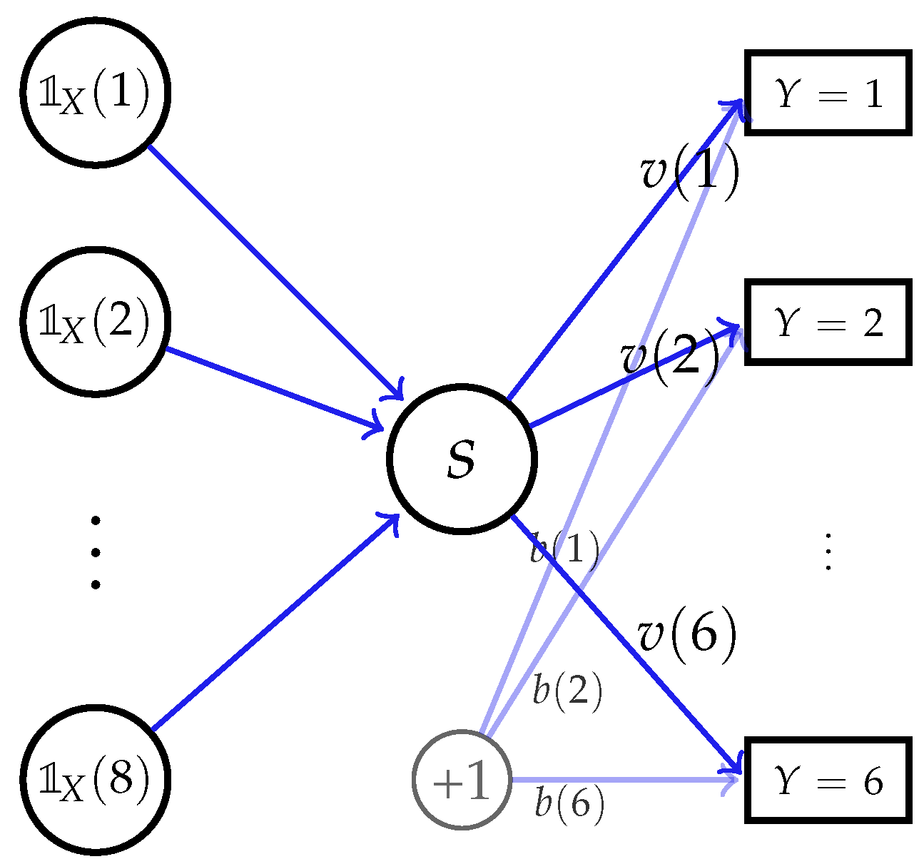
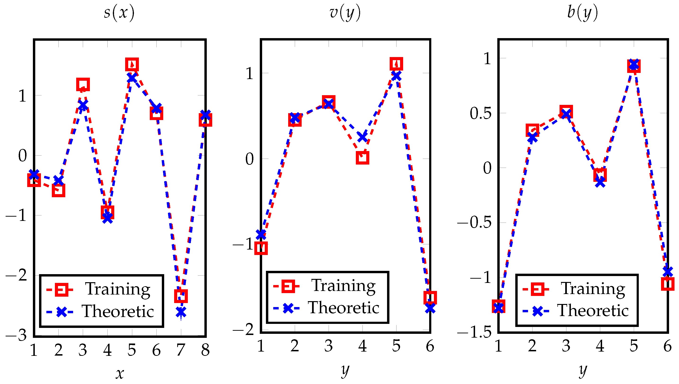
We first validate Theorem 4, the optimal feature extracted by network with ideal expressive power. Here, we consider the discrete data with alphabet sizes, $\left|\mathcal{X}\right|=8$ and $\left|\mathcal{Y}\right|=6$, and construct the network as shown in Figure 3. Specifically, the network input is the one-hot encoding of X, i.e., $[1_X\left(1\right),\dots ,1_X{\left(\right|\mathcal{X}\left|\right)]}^{\mathrm{T}}$, where $1_X\left(x\right)$ takes one if and only if $X=x$, and takes zero otherwise. Then, the feature $s\left(X\right)$ is generated by a linear layer, with sigmoid function used as the activation function. For ease of comparison and presentation, we set feature dimension to $k=1$, since otherwise the optimal feature (cf. Theorem 4) lies in a subspace and is non-unique. It can be verified that this network has ideal expressive power, i.e., with proper weights in the first layer, $s\left(X\right)$ can express any desired function up to scaling and shifting.

To compare the result trained by the neural network and that in Theorem 4, we first randomly generate a distribution $P_{XY}$, and then draw independently $n=$ 100,000 pairs of $(X,Y)$ samples. We then train the network using batch gradient descent, where we have applied Nesterov momentum [43] with the momentum hyperparameter being 0.9. In addition, we set the learning rate to 4 with a decay factor of 0.01 and clip gradients with norm exceeding 0.5. After training, the learned values of $s\left(x\right),v\left(y\right)$ and $b\left(y\right)$ are shown in Figure 4 and compared with theoretical results. From the figure, we can observe that the training results match our theoretical analyses.

3.4.2. Experimental Validation of Theorem 5

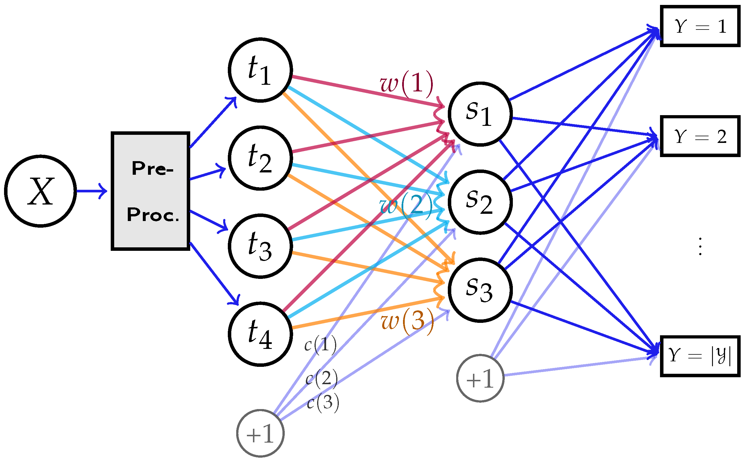
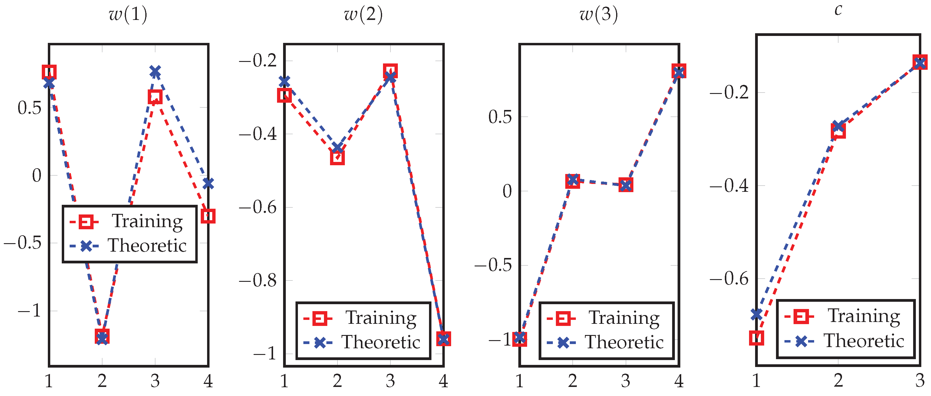
In addition, we validate Theorem 5 by the neural network depicted in Figure 5, with the same settings of $X,Y$. Specifically, the number of neurons in hidden layers are set to $m=4$ and $k=3$, where $t\left(X\right)$ is randomly generated from X, and we have chosen sigmoid function as the activation function $\sigma (·)$ to generate $s\left(x\right)$. We then fix the weights and bias at the output layer and train the weights $w\left(1\right),w\left(2\right)$, $w\left(3\right)$ and bias c in the hidden layer to optimize the log-loss. Specifically, we use the batch gradient descent with the Nesterov momentum hyperparameter being 0.9. In addition, we set the learning rate to 4 with a decay factor of ${10}^{-6}$ and clip gradients with norm exceeding 0.1. After training, Figure 6 shows the matching between the learned results and the corresponding theoretical values.

3.4.3. Experimental Validation of H-Score

To validate H-score as a performance measure for extracted features, we compare the H-score and classification accuracy of DNNs on image classification tasks. Specifically, we use the ImageNet Large Scale Visual Recognition Challenge 2012 (ILSVRC2012) [22] dataset as the dataset and extract features using several deep neural networks with representative architectures designs [44,45,46,47,48,49]. After training the feature extractors on the ILSVRC2012 training set, we then compute the H-score of the feature in the last hidden layer, as well as the classification accuracies on ILSVRC2012 validation set (here, we use ILSVRC2012 validation set for testing, as the labels in ILSVRC2012 testing set have not been publicly released). The results are summarized in

Table 1. Classification accuracy and H-score for different DNN models on ImageNet dataset, where “Paras” indicates the number of parameters (in millions) in the model and $H_{\mathrm{AIC}}$ represents the AIC-corrected H-score.

DNN Model	Paras [$\times {10}^6$]	$\mathit{H}\left(\mathit{s}\right)$	${\mathit{H}}_{\mathbf{AIC}}\left(\mathit{s}\right)$	Accuracy [%]
VGG16 [44]	138.4	148.3	41.9	64.2
VGG19 [44]	143.7	152.7	42.2	64.7
MobileNet [45]	4.3	45.9	42.6	68.4
DenseNet121 [46]	8.1	59.5	53.3	71.4
DenseNet169 [46]	14.3	81.2	70.2	73.6
DenseNet201 [46]	20.2	89.1	73.5	74.4
Xception [47]	22.9	179.8	162.2	77.5
InceptionV3 [48]	23.9	181.2	162.9	76.3
InceptionResNetV2 [49]	55.9	241.1	198.1	79.1

, where $H_{\mathrm{AIC}}\left(s\right)$ is the AIC-corrected H-score as defined in (27), with $n_{\mathrm{p}}$ being the number of model parameters, and $n_{\mathrm{s}}=$ 1,300,000 corresponding to the number of training samples in ImageNet. The AIC-corrected H-score is consistent with the classification accuracy, which validates the effectiveness of H-score as a measurement of neural networks.

4. Discussion

Our characterization gives an information-theoretic interpretation of the feature extraction process in DNNs, which also provides a practical performance measure for scoring neural networks. Different from empirical studies focusing on specific datasets [7], our development is based on the probability distribution space, which is more general and can also provide theoretic insights. Moreover, the information-theoretic framework allows us to obtain direct operational meaning and better interpretations for the solutions, compared with optimization-based theoretical characterizations, e.g., [11,13].

As a first step in establishing a rigorous framework for DNN analysis, the present work can be extended in both theoretical and practical aspects. From the theoretical perspective, one extension is to investigate the analytical properties for general DNNs, using the theoretic insights obtained from local analysis regime. For example, it was shown in [50] that the symmetry between feature and weights in DNNs established in the local analysis regime (cf. Section 3.2.1) also holds for general probability distributions. Another extension is to apply the framework to investigate the optimal feature for structured data or network, e.g., data with sparsity structure [51].

From the practical perspective, in addition to the demonstrated example of evaluating existing DNN models (cf. Section 3.4.3), the H-score can also be used as an objective function in designing learning algorithms. In particular, such usages have been illustrated in multi-modal learning [52] and transfer learning [53] tasks.

5. Conclusions

In this paper, we apply the local information geometric analysis and provide an information-theoretic interpretation to the feature extraction scheme in DNNs. We first establish an information metric for features in inference tasks by formalizing the information-theoretic feature selection problem. In addition, we demonstrate that the features extracted by DNNs coincide with the information-theoretically optimal feature, with the same metric measuring the performance of features, called H-score. Furthermore, we discuss the usage of the H-score for measuring the effectiveness of DNNs. Our framework demonstrates a connection between the practical deep learning implementations and information-theoretic characterizations, which can provide theoretical insights for DNN analysis and learning algorithm designs.

References

- He, K.; Zhang, X.; Ren, S.; Sun, J. Deep residual learning for image recognition. In Proceedings of the IEEE Conference on Computer Vision and Pattern Recognition, Las Vegas, NV, USA, 26 June–1 July 2016; pp. 770–778. [Google Scholar]
- Devlin, J.; Chang, M.W.; Lee, K.; Toutanova, K. BERT: Pre-training of Deep Bidirectional Transformers for Language Understanding. In Proceedings of the 2019 Conference of the North American Chapter of the Association for Computational Linguistics: Human Language Technologies, Minneapolis, MN, USA, 3–5 June 2019; Volume 1 (Long and Short Papers). Association for Computational Linguistics: Minneapolis, MN, USA, 2019; pp. 4171–4186. [Google Scholar]
- Brown, T.; Mann, B.; Ryder, N.; Subbiah, M.; Kaplan, J.D.; Dhariwal, P.; Neelakantan, A.; Shyam, P.; Sastry, G.; Askell, A.; et al. Language Models are Few-Shot Learners. In Advances in Neural Information Processing Systems; Larochelle, H., Ranzato, M., Hadsell, R., Balcan, M.F., Lin, H., Eds.; Curran Associates, Inc.: Red Hook, NY, USA, 2020; Volume 33, pp. 1877–1901. [Google Scholar]
- Silver, D.; Huang, A.; Maddison, C.J.; Guez, A.; Sifre, L.; Van Den Driessche, G.; Schrittwieser, J.; Antonoglou, I.; Panneershelvam, V.; Lanctot, M.; et al. Mastering the game of Go with deep neural networks and tree search. Nature 2016, 529, 484–489. [Google Scholar] [CrossRef]
- Arulkumaran, K.; Cully, A.; Togelius, J. Alphastar: An evolutionary computation perspective. In Proceedings of the Genetic and Evolutionary Computation Conference Companion, Prague, Czech Republic, 13–17 July 2019; pp. 314–315. [Google Scholar]
- MacKay, D.J.C. Information Theory, Inference, and Learning Algorithms; Cambridge University Press: Cambridge, UK, 2003; ISBN 9780521642989. [Google Scholar]
- Zintgraf, L.M.; Cohen, T.S.; Adel, T.; Welling, M. Visualizing Deep Neural Network Decisions: Prediction Difference Analysis. In Proceedings of the 5th International Conference on Learning Representations, ICLR 2017, Toulon, France, 24–26 April 2017. [Google Scholar]
- Papyan, V.; Han, X.; Donoho, D.L. Prevalence of neural collapse during the terminal phase of deep learning training. Proc. Natl. Acad. Sci. USA 2020, 117, 24652–24663. [Google Scholar] [CrossRef]
- Adebayo, J.; Gilmer, J.; Muelly, M.; Goodfellow, I.; Hardt, M.; Kim, B. Sanity Checks for Saliency Maps. In Advances in Neural Information Processing Systems; Bengio, S., Wallach, H., Larochelle, H., Grauman, K., Cesa-Bianchi, N., Garnett, R., Eds.; Curran Associates, Inc.: Red Hook, NY, USA, 2018; Volume 31. [Google Scholar]
- Guidotti, R.; Monreale, A.; Ruggieri, S.; Turini, F.; Giannotti, F.; Pedreschi, D. A survey of methods for explaining black box models. ACM Comput. Surv. (CSUR) 2018, 51, 1–42. [Google Scholar] [CrossRef] [Green Version]
- Jacot, A.; Gabriel, F.; Hongler, C. Neural Tangent Kernel: Convergence and Generalization in Neural Networks. In Advances in Neural Information Processing Systems; Bengio, S., Wallach, H., Larochelle, H., Grauman, K., Cesa-Bianchi, N., Garnett, R., Eds.; Curran Associates, Inc.: Red Hook, NY, USA, 2018; Volume 31. [Google Scholar]
- Mei, S.; Montanari, A.; Nguyen, P.M. A mean field view of the landscape of two-layer neural networks. Proc. Natl. Acad. Sci. USA 2018, 115, E7665–E7671. [Google Scholar] [CrossRef] [Green Version]
- Arora, S.; Du, S.; Hu, W.; Li, Z.; Wang, R. Fine-grained analysis of optimization and generalization for overparameterized two-layer neural networks. In Proceedings of the International Conference on Machine Learning, PMLR, Long Beach, CA, USA, 9–15 June 2019; pp. 322–332. [Google Scholar]
- Cover, T.M.; Thomas, J.A. Elements of Information Theory; John Wiley & Sons: Hoboken, NJ, USA, 2012. [Google Scholar]
- Huang, S.L.; Xu, X.; Zheng, L.; Wornell, G.W. An information theoretic interpretation to deep neural networks. In Proceedings of the 2019 IEEE International Symposium on Information Theory (ISIT), Paris, France, 7–12 July 2019; pp. 1984–1988. [Google Scholar]
- Tishby, N.; Zaslavsky, N. Deep learning and the information bottleneck principle. In Proceedings of the Information Theory Workshop (ITW), Jerusalem, Israel, 26 April–1 May 2015; pp. 1–5. [Google Scholar]
- Goldfeld, Z.; Polyanskiy, Y. The information bottleneck problem and its applications in machine learning. IEEE J. Sel. Areas Inf. Theory 2020, 1, 19–38. [Google Scholar] [CrossRef]
- Huang, S.L.; Makur, A.; Zheng, L.; Wornell, G.W. An information-theoretic approach to universal feature selection in high-dimensional inference. In Proceedings of the 2017 IEEE International Symposium on Information Theory (ISIT), Aachen, Germany, 25–30 June 2017; pp. 1336–1340. [Google Scholar]
- Arjovsky, M.; Chintala, S.; Bottou, L. Wasserstein generative adversarial networks. In Proceedings of the International Conference on Machine Learning, PMLR, Sydney, Australia, 6–11 August 2017; pp. 214–223. [Google Scholar]
- Saxe, A.M.; Bansal, Y.; Dapello, J.; Advani, M.; Kolchinsky, A.; Tracey, B.D.; Cox, D.D. On the information bottleneck theory of deep learning. J. Stat. Mech. Theory Exp. 2019, 2019, 124020. [Google Scholar] [CrossRef]
- Goodfellow, I.; Bengio, J.; Courville, A. Deep Learning; MIT Press: Cambridge, MA, USA, 2017. [Google Scholar]
- Olga, R.; Jia, D.; Hao, S.; Jonathan, K.; Sanjeev, S.; Sean, M.; Zhiheng, H.; Andrej, K.; Aditya, K.; Michael, B.; et al. ImageNet Large Scale Visual Recognition Challenge. Int. J. Comput. Vis. 2015, 115, 211–252. [Google Scholar] [CrossRef] [Green Version]
- Huang, S.L.; Zheng, L. Linear information coupling problems. In Proceedings of the 2012 IEEE International Symposium on Information Theory Proceedings, Cambridge, MA, USA, 1–6 July 2012; pp. 1029–1033. [Google Scholar]
- Huang, S.L.; Makur, A.; Wornell, G.W.; Zheng, L. On universal features for high-dimensional learning and inference. arXiv 2019, arXiv:1911.09105. [Google Scholar]
- Hirschfeld, H.O. A connection between correlation and contingency. Proc. Camb. Phil. Soc. 1935, 31, 520–524. [Google Scholar] [CrossRef]
- Gebelein, H. Das statistische problem der Korrelation als variations-und Eigenwertproblem und sein Zusammenhang mit der Ausgleichungsrechnung. Z. Angew. Math. Mech. 1941, 21, 364–379. [Google Scholar] [CrossRef]
- Rényi, A. On Measures of Dependence. Acta Math. Acad. Sci. Hung. 1959, 10, 441–451. [Google Scholar] [CrossRef]
- du Pin Calmon, F.; Makhdoumi, A.; Médard, M.; Varia, M.; Christiansen, M.; Duffy, K.R. Principal inertia components and applications. IEEE Trans. Inf. Theory 2017, 63, 5011–5038. [Google Scholar] [CrossRef] [Green Version]
- Hsu, H.; Asoodeh, S.; Salamatian, S.; Calmon, F.P. Generalizing bottleneck problems. In Proceedings of the 2018 IEEE International Symposium on Information Theory (ISIT), Vail, CO, USA, 17–22 June 2018; pp. 531–535. [Google Scholar]
- Hsu, H.; Salamatian, S.; Calmon, F.P. Correspondence analysis using neural networks. In Proceedings of the 22nd International Conference on Artificial Intelligence and Statistics, PMLR, Okinawa, Japan,, 16–18 April 2019; pp. 2671–2680. [Google Scholar]
- Anantharam, V.; Gohari, A.; Kamath, S.; Nair, C. On hypercontractivity and a data processing inequality. In Proceedings of the 2014 IEEE International Symposium on Information Theory, Honolulu, HI, USA,, 29 June–4 July 2014; pp. 3022–3026. [Google Scholar]
- Raginsky, M. Strong data processing inequalities and Φ-Sobolev inequalities for discrete channels. IEEE Trans. Inf. Theory 2016, 62, 3355–3389. [Google Scholar] [CrossRef] [Green Version]
- Polyanskiy, Y.; Wu, Y. Strong data-processing inequalities for channels and Bayesian networks. In Convexity and Concentration; Springer: Berlin/Heidelberg, Germany, 2017; pp. 211–249. [Google Scholar]
- Greenacre, M.J. Theory and Applications Of Correspondence Analysis; Academic Press: London, UK, 1984. [Google Scholar]
- Wang, H.; Vo, L.; Calmon, F.P.; Médard, M.; Duffy, K.R.; Varia, M. Privacy with estimation guarantees. IEEE Trans. Inf. Theory 2019, 65, 8025–8042. [Google Scholar] [CrossRef]
- Breiman, L.; Friedman, J.H. Estimating Optimal Transformations for Multiple Regression and Correlation. J. Am. Stat. Assoc. 1985, 80, 614–619. [Google Scholar]
- Sutskever, I.; Vinyals, O.; Le, Q.V. Sequence to sequence learning with neural networks. In Proceedings of the Advances in Neural Information Processing Systems, Montreal, QC, Canada, 8–13 December 2014; pp. 3104–3112. [Google Scholar]
- Hochreiter, S.; Schmidhuber, J. Long short-term memory. Neural Comput. 1997, 9, 1735–1780. [Google Scholar] [CrossRef]
- Hastie, T.; Tibshirani, R.; Friedman, J. Neural Networks. In The Elements of Statistical Learning: Data Mining, Inference, and Prediction; Springer: New York, NY, USA, 2009; pp. 389–416. [Google Scholar] [CrossRef]
- Cybenko, G. Approximation by superpositions of a sigmoidal function. Math. Control. Signals Syst. 1989, 2, 303–314. [Google Scholar] [CrossRef]
- Stoer, J.; Bulirsch, R. Introduction to Numerical Analysis; Springer Science & Business Media: Berlin/Heidelberg, Germany, 2013; Volume 12. [Google Scholar]
- Alain, G.; Bengio, Y. Understanding intermediate layers using linear classifier probes. In Proceedings of the 5th International Conference on Learning Representations, ICLR 2017, Toulon, France, 24–26 April 2017. [Google Scholar]
- Sutskever, I.; Martens, J.; Dahl, G.; Hinton, G. On the importance of initialization and momentum in deep learning. In Proceedings of the International Conference on Machine Learning, PMLR, Atlanta, GA, USA, 17–19 June 2013; pp. 1139–1147. [Google Scholar]
- Simonyan, K.; Zisserman, A. Very Deep Convolutional Networks for Large-Scale Image Recognition. In Proceedings of the 3rd International Conference on Learning Representations, ICLR 2015, San Diego, CA, USA, 7–9 May 2015; Bengio, Y., LeCun, Y., Eds.; Conference Track Proceedings. [Google Scholar]
- Howard, A.G.; Zhu, M.; Chen, B.; Kalenichenko, D.; Wang, W.; Weyand, T.; Andreetto, M.; Adam, H. Mobilenets: Efficient convolutional neural networks for mobile vision applications. arXiv 2017, arXiv:1704.04861. [Google Scholar]
- Huang, G.; Liu, Z.; Weinberger, K.Q.; van der Maaten, L. Densely connected convolutional networks. In Proceedings of the IEEE Conference on Computer Vision and Pattern Recognition, Honolulu, HI, USA, 21–29 July 2017; Volume 1, p. 3. [Google Scholar]
- Chollet, F. Xception: Deep learning with depthwise separable convolutions. In Proceedings of the IEEE Conference on Computer Vision and Pattern Recognition, Honolulu, HI, USA, 21–29 July 2017; pp. 1251–1258. [Google Scholar]
- Szegedy, C.; Vanhoucke, V.; Ioffe, S.; Shlens, J.; Wojna, Z. Rethinking the inception architecture for computer vision. In Proceedings of the IEEE Conference on Computer Vision and Pattern Recognition, Las Vegas, NV, USA,, 26 June–1 July 2016; pp. 2818–2826. [Google Scholar]
- Szegedy, C.; Ioffe, S.; Vanhoucke, V.; Alemi, A.A. Inception-v4, Inception-ResNet and the Impact of Residual Connections on Learning. In Proceedings of the AAAI, San Francisco, CA, USA, 4–9 February 2017; pp. 4278–4284. [Google Scholar]
- Xu, X.; Huang, S.L.; Zheng, L.; Zhang, L. The geometric structure of generalized softmax learning. In Proceedings of the 2018 IEEE Information Theory Workshop (ITW), Guangzhou, China, 25–29 November 2018; pp. 1–5. [Google Scholar]
- Wen, W.; Wu, C.; Wang, Y.; Chen, Y.; Li, H. Learning structured sparsity in deep neural networks. Adv. Neural Inf. Process. Syst. 2016, 29, 2074–2082. [Google Scholar]
- Wang, L.; Wu, J.; Huang, S.L.; Zheng, L.; Xu, X.; Zhang, L.; Huang, J. An efficient approach to informative feature extraction from multimodal data. In Proceedings of the AAAI Conference on Artificial Intelligence, Honolulu, HI, USA, 27 January–1 February 2019; Volume 33, pp. 5281–5288. [Google Scholar]
- Lee, J.; Sattigeri, P.; Wornell, G. Learning new tricks from old dogs: Multi-source transfer learning from pre-trained networks. Adv. Neural Inf. Process. Syst. 2019, 32, 4370–4380. [Google Scholar]
- Dembo, A.; Zeitouni, O. Large Deviations Techniques and Applications; Corrected Reprint of the Second (1998) Edition; Stochastic Modelling and Applied Probability; Springer: Berlin/Heidelberg, Germany, 2010; p. 38. [Google Scholar]
- Sason, I.; Verdú, S. f-divergence Inequalities. IEEE Trans. Inf. Theory 2016, 62, 5973–6006. [Google Scholar] [CrossRef]
- Eckart, C.; Young, G. The approximation of one matrix by another of lower rank. Psychometrika 1936, 1, 211–218. [Google Scholar] [CrossRef]
Figure 1.
A deep neural network that uses data X to predict Y. All hidden layers together map the input data X to k-dimensional feature . Then, the probabilistic prediction of Y is computed from , and , where v and bias b are the weights and bias in the last layer.
Figure 2.
A multi-layer neural network, where the expressive power of the feature mapping is restricted by the hidden representation t. All hidden layers previous to t are fixed, represented by the “pre-processing” module.
Figure 3.
A simple neural network with ideal expressive power, which can generate any dimensional feature s of X by tuning the weights in the first layer.
Figure 4.
The trained feature s, weights v, and bias b of the network in Figure 3, which are compared with the corresponding theoretical results to show their coincidences.
Figure 5.
The designed network for validating the impact of network structure on feature extraction, with and neurons in two hidden layers. Our goal is to compare the learned weights , and bias c in the hidden layer with our theoretic characterizations in Section 3.2.2.
Figure 6.
The trained weights w and bias c of the network in Figure 5, which are compared with the corresponding theoretical results to show their coincidences.