
Numerical Solutions of Variable Coefficient Higher-Order Partial Differential Equations Arising in Beam Models

 and
and
Abstract
:1. Introduction
2. Motivation
3. Haar Wavelets and Their Integrals
Function Approximation
4. Description of the Method
Note
5. Stability
6. Illustrative Examples
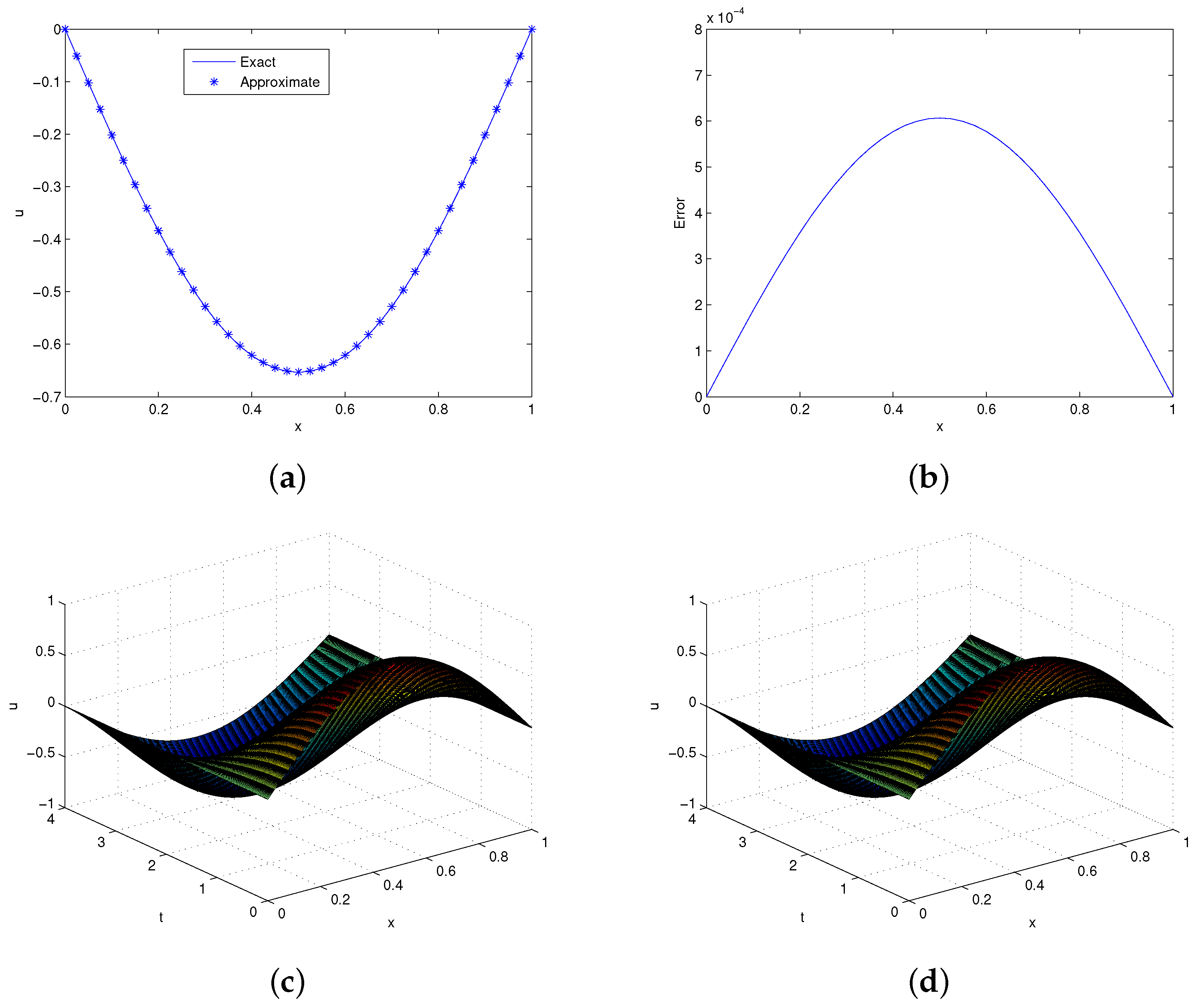
6.1. Problem 5.1
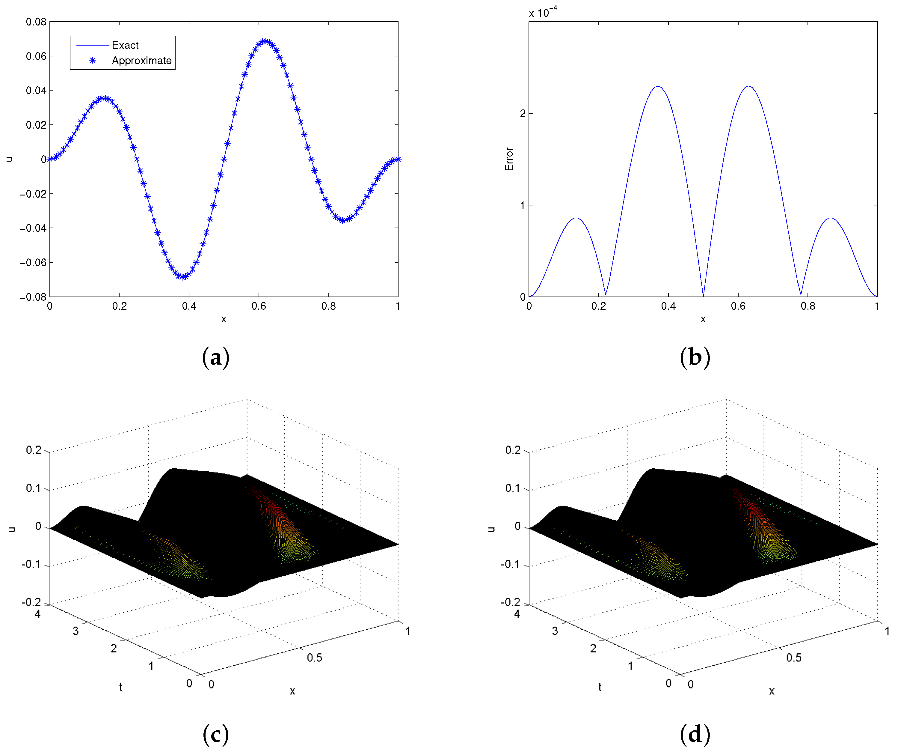
6.2. Problem 5.2
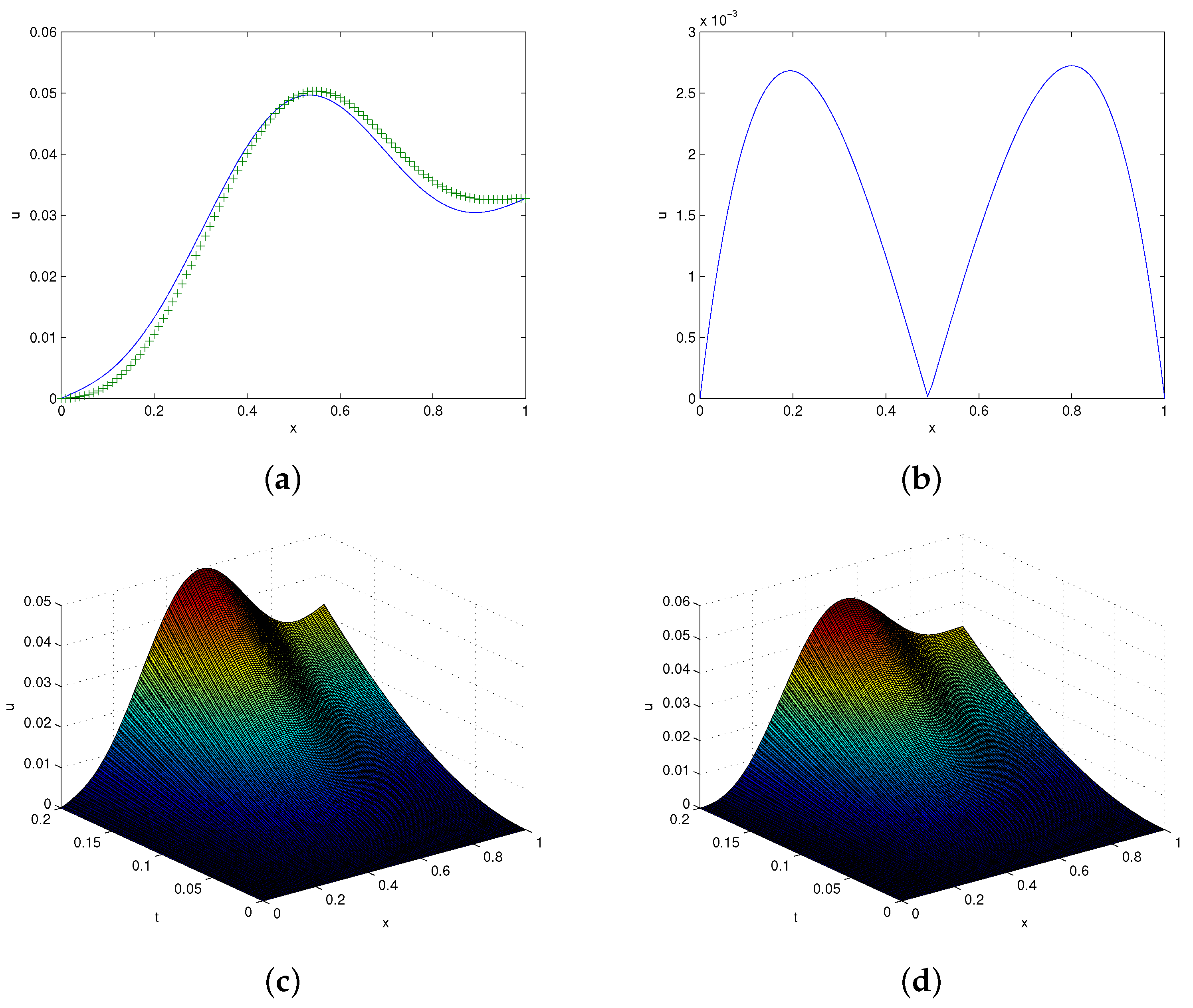
6.3. Problem 5.3
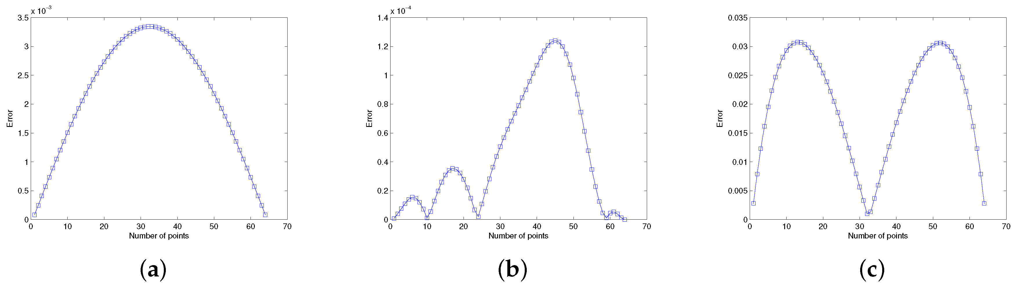
7. Initial Disturbance and Noisy Data
8. Conclusions
Author Contributions
Funding
Institutional Review Board Statement
Informed Consent Statement
Data Availability Statement
Acknowledgments
Conflicts of Interest
References
- Ahn, J.; Stewart, D.E. An Euler–Bernoulli beam with dynamic frictionless contact: Penalty approximation and existence. Numer. Funct. Anal. Optim. 2007, 28, 1003–1026. [Google Scholar] [CrossRef]
- Kunisch, K.; Graif, E. Parameter estimation for the Euler–Bernoulli beam. Mat. Apficada Comput. 1985, 4, 95–124. [Google Scholar]
- Timoshenko, S.P.; Gere, J.M. Theory of Elastic Stability; McGraw-Hill: New York, NY, USA, 1961. [Google Scholar]
- Wazwaz, A.M. Analytic treatment for variable coefficient fourth-order parabolic partial differential equations. Appl. Math. Comput. 2001, 123, 219–227. [Google Scholar] [CrossRef]
- Liu, Y.; Gurram, C.S. The use of Hes variational iteration method for obtaining the free vibration of an EulerBernoulli beam. Math. Comput. Model. 2009, 50, 1545–1552. [Google Scholar] [CrossRef]
- Jain, M.K.; Iyengar, S.R.K.; Lone, A.G. Higher order difference formulas for a fourth order parabolic partial differential equation. Int. J. Numer. Methods Eng. 1976, 10, 1357–1367. [Google Scholar] [CrossRef]
- Evans, D.J. A stable explicit method for the finite difference solution of a fourth order parabolic partial differential equation. Comput. J. 1965, 8, 280–287. [Google Scholar] [CrossRef] [Green Version]
- Conte, S.D. A stable implicit finite difference approximation to a fourth order parabolic equation. J. Assoc. Comput. Mech. 1957, 4, 18–23. [Google Scholar] [CrossRef]
- Richtmyer, R.D.; Morton, K.W. Difference Methods for Initial Value Problems, 2nd ed.; Wiley-Interscience: NewYork, NY, USA, 1967. [Google Scholar]
- Crandall, S.H. Numerical treatment of a fourth order partial differential equations. J. Assoc. Comput. Mech. 1954, 1, 111–118. [Google Scholar] [CrossRef]
- Danaee, A.; Khan, A.; Khan, I.; Aziz, T.; Evans, D.J. Hopscotch procedure for a fourthorder parabolic partial differential equation. Math. Comput. Simul. 1982, 24, 326–329. [Google Scholar] [CrossRef]
- Aziz, T.; Khan, A.; Rashidinia, J. Spline methods for the solution of fourth-order parabolic partial differential equations. Appl. Math. Comput. 2005, 167, 153–166. [Google Scholar] [CrossRef]
- Rashidinia, J.; Mohammadi, R. Sextic spline solution of variable coefficient fourthorder parabolic equations. Int. J. Comput. Math. 2010, 87, 3443–3454. [Google Scholar] [CrossRef]
- Ahmad, I.; Hijaz, A.; Inc, M.; Rezazadeh, H.; Akbar, M.A.; Khater, M.M.A.; Akinyemi, L.; Jhangeer, A. Solution of fractional-order Korteweg-de Vries and Burgers’ equations utilizing local meshless method. J. Ocean Eng. Sci. 2021, 1–12. [Google Scholar] [CrossRef]
- Senol, M.; Akinyemi, L.; Ata, A.; Iyiola, O.S. SApproximate and generalized solutions of conformable type Coudrey–Dodd–Gibbon–Sawada–Kotera equation. Int. J. Mod. Phy. B 2021, 35, 2150021. [Google Scholar] [CrossRef]
- Akinyemi, L.; Iyiola, O.S. Analytical Study of (3+1)-Dimensional Fractional-Reaction Diffusion Trimolecular Models. Int. J. Appl. Comp. Math. 2021, 7, 1–24. [Google Scholar] [CrossRef]
- Akinyemi, L.; Veeresha, P.; Ajibola, S.O. Numerical simulation for coupled nonlinear Schrödinger–Korteweg–de Vries and Maccari systems of equations. Mod. Phy. Lett. B 2021, 35, 2150339. [Google Scholar] [CrossRef]
- Jiwari, R. Barycentric rational interpolation and local radial basis functions based numerical algorithms for multidimensional sine-Gordon equation. Num. Meth. Part. Diff. Eqs. 2021, 37, 1965–1992. [Google Scholar] [CrossRef]
- Bertoluzza, S. An adaptive collocation method based on interpolating wavelets. In Multi-Scale Wavelet Methods for Partial Differential Equations; Dahmen, W., Kurdila, A.J., Oswald, P., Eds.; Academic Press: San Diego, CA, USA, 1977; pp. 109–135. [Google Scholar]
- Beylkin, G.; Keiser, J.M. An adaptive pseudo-wavelet approach for solving nonlinear partial differential equations. In Multi-Scale Wavelet Methods for Partial Differential Equations; Dahmen, W., Kurdila, A.J., Oswald, P., Eds.; Academic Press: San Diego, CA, USA, 1977; pp. 137–197. [Google Scholar]
- Cattani, C. Haar wavelet splines. J. Interdiscip. Math. 2001, 4, 35–47. [Google Scholar] [CrossRef]
- Cattani, C. Haar wavelets based technique in evolution problems. Proc. Estonian Acad. Sci. Phys. Math. 2004, 1, 45–63. [Google Scholar] [CrossRef]
- Chen, C.F.; Hasio, C.H. Haar wavelet method for solving lumped and distributedparameter systems. IEE Proc. Number Control Theory Appl. 1997, 144, 87–94. [Google Scholar] [CrossRef] [Green Version]
- Lepik, U. Numerical solution of evolution equations by the Haar wavelet method. Appl. Math. Comput. 2007, 185, 695–704. [Google Scholar] [CrossRef]
- Lepik, U. Solving PDEs with the aid of two-dimensional Haar wavelets. Comput. Math. Appl. 2011, 61, 1873–1879. [Google Scholar] [CrossRef] [Green Version]
- Jiwari, R. A Haar wavelet quasilinearization approach for numerical simulation of Burgers equation. Comput. Phy. Comm. 2012, 183, 2413–2423. [Google Scholar] [CrossRef]
- Mittal, R.C.; Kaur, H.; Mishra, V. Haar Wavelet Based Numerical Investigation of Coupled Viscous Burgers equation. Int. J. Comput. Appl. 2015, 92, 1643–1659. [Google Scholar] [CrossRef]
- Oruç, Ö.; Bulut, F.; Esen, A. A Haar wavelet-finite difference hybrid method for the numerical solution of the modified Burgers equation. J. Math. Chem. 2015, 53, 1592–1607. [Google Scholar] [CrossRef]
- Oruç, Ö.; Bulut, F.; Esen, A. Numerical solution of the KdV equation by Haar wavelet method. Pramana J. Phys. 2016, 87, 94. [Google Scholar] [CrossRef]
- Kumar, M.; Pandit, S. A composite numerical scheme for the numerical simulation of coupled Burgers equation. Comput. Phys. Commun. 2014, 185, 809–817. [Google Scholar] [CrossRef]
- Arbabi, S.; Nazari, A.; Darvishi, M.T. A semi-analytical solution of Hunter-Saxton equation. Optik 2016, 127, 5255–5258. [Google Scholar] [CrossRef]
- Arbabi, S.; Nazari, A.; Darvishi, M.T. A semi-analytical solution of foam drainage equation by Haar wavelets method. Optik 2016, 127, 5443–5447. [Google Scholar] [CrossRef]
- Arbabi, S.; Nazari, A.; Darvishi, M.T. A two-dimensional Haar wavelets method for solving systems of PDEs. Appl. Math. Comp. 2017, 292, 33–46. [Google Scholar] [CrossRef]
- Mittal, R.C.; Pandit, S. Numerical simulation of unsteady squeezing nanofluid and heat flow between two parallel plates using wavelets. Int. J. Ther. Sci. 2017, 118, 417–422. [Google Scholar] [CrossRef]
- Jiwari, R. A hybrid numerical scheme for the numerical solution of the Burgers’ equation. Comput. Phys. Commun. 2015, 188, 59–67. [Google Scholar] [CrossRef]
- Pandit, S.; Mittal, R.C. A numerical algorithm based on scale-3 Haar wavelets for fractional advection dispersion equation. Eng. Comput. 2020, 38, 1706–1724. [Google Scholar] [CrossRef]
- Pandit, S.; Jiwari, R.; Bedi, K.; Koksal, M.E. Haar wavelets operational matrix based algorithm for computational modeling of hyperbolic type wave equations. Eng. Comput. 2017, 34, 2793–2814. [Google Scholar] [CrossRef]
- Haq, S.; Ghafoor, A. An efficient numerical algorithm for multi-dimensional time dependent partial differential equations. Comput. Math. Appl. 2018, 75, 2723–2734. [Google Scholar] [CrossRef]
- Mittal, R.C.; Jain, R.K. B-Splines methods with redefined basis functions for solving fourth order parabolic partial differential equations. Appl. Math. Comput. 2011, 217, 9741–9755. [Google Scholar] [CrossRef]
- Caglar, H.; Caglar, N. Fifth-degree B-spline solution for a fourth-order parabolic partial differential equations. Appl. Math. Comput. 2008, 201, 597–603. [Google Scholar] [CrossRef]
- Mohammadi, R. Sextic B-spline collocation method for solving Euler–Bernoulli Beam Models. Appl. Math. Comput. 2014, 241, 151–166. [Google Scholar] [CrossRef]
- Shivanian, E.; Jafarabadi, A. Inverse Cauchy problem of annulus domains in the framework of spectral meshless radial point interpolation. Eng. Comput. 2017, 33, 431–442. [Google Scholar] [CrossRef]
- Solodusha, S.V.; Mokry, I.V. A numerical solution of one class of Volterra integral equations of the first kind in terms of the machine arithmetic features. Bull. SUSU MMCS 2016, 9, 119–129. [Google Scholar] [CrossRef]


| Methods | Points | t | |||||
|---|---|---|---|---|---|---|---|
| Present | 64 | 0.02 | 6.54 × 10 | 1.24 × 10 | 1.71 × 10 | 2.01 × 10 | 2.11 × 10 |
| 64 | 0.05 | 5.22 × 10 | 9.94 × 10 | 1.36 × 10 | 1.60 × 10 | 1.69 × 10 | |
| 64 | 1 | 7.14 × 10 | 1.35 × 10 | 1.87 × 10 | 2.20 × 10 | 2.31 × 10 | |
| 128 | 0.02 | 2.60 × 10 | 4.94 × 10 | 6.81 × 10 | 8.00 × 10 | 8.42 × 10 | |
| 128 | 0.05 | 2.59 × 10 | 4.94 × 10 | 6.80 × 10 | 7.99 × 10 | 8.40 × 10 | |
| 128 | 1 | 6.83 × 10 | 1.29 × 10 | 1.78 × 10 | 2.10 × 10 | 2.21 × 10 | |
| Mittal [39] | 91 | 0.02 | 3.20 × 10 | 6.08 × 10 | 8.37 × 10 | 9.84 × 10 | 1.04 × 10 |
| 91 | 0.05 | 3.59 × 10 | 6.83 × 10 | 9.39 × 10 | 1.10 × 10 | 1.16 × 10 | |
| 91 | 1 | 6.32 × 10 | 1.20 × 10 | 1.65 × 10 | 1.94 × 10 | 2.04 × 10 | |
| 181 | 0.02 | 3.55 × 10 | 6.76 × 10 | 9.30 × 10 | 1.09 × 10 | 1.15 × 10 | |
| 181 | 0.05 | 3.99 × 10 | 7.58 × 10 | 1.04 × 10 | 1.23 × 10 | 1.29 × 10 | |
| 181 | 1 | 7.00 × 10 | 1.33 × 10 | 1.83 × 10 | 2.16 × 10 | 2.27 × 10 | |
| Caglar [40] | 121 | 0.02 | 4.80 × 10 | 9.70 × 10 | 1.40 × 10 | 1.90 × 10 | 2.40 × 10 |
| 191 | 0.02 | 5.20 × 10 | 2.10 × 10 | 3.10 × 10 | 4.20 × 10 | 5.20 × 10 | |
| 521 | 0.02 | 4.90 × 10 | 9.90 × 10 | 1.40 × 10 | 1.90 × 10 | 2.40 × 10 | |
| Aziz et al. [12] | 20 | 0.05 | 9.30 × 10 | 8.00 × 10 | 2.80 × 10 | 1.00 × 10 | 2.70 × 10 |
| Rashidinia [13] | 20 | 0.05 | 2.91 × 10 | 1.73 × 10 | 1.60 × 10 | 2.23 × 10 | 2.60 × 10 |
| Mohammadi [41] | 40 | 0.05 | 2.96 × 10 | 1.77 × 10 | 1.64 × 10 | 2.28 × 10 | 2.65 × 10 |
| Problem 4.1 | |||
|---|---|---|---|
| Rate | |||
| 2 | 1/100 | 90,568 × 10 | |
| 3 | 1/200 | 2.4428 × 10 | 1.8904 |
| 4 | 1/400 | 6.8223 × 10 | 1.8402 |
| 5 | 1/800 | 2.0398 × 10 | 1.7418 |
| Methods | Points | |||||||
|---|---|---|---|---|---|---|---|---|
| Present | 32 | 0.001 | 1.76 × 10 | 5.72 × 10 | 1.80 × 10 | 2.14 × 10 | 2.87 × 10 | 2.39 × 10 |
| 64 | 0.001 | 1.72 × 10 | 5.75 × 10 | 1.48 × 10 | 1.90 × 10 | 2.95 × 10 | 6.13 × 10 | |
| [41] | 100 | 0.01 | 1.78 × 10 | 5.85 × 10 | 1.57 × 10 | 2.00 × 10 | 2.95 × 10 | 1.60 × 10 |
| 200 | 0.005 | 2.38 × 10 | 7.80 × 10 | 2.09 × 10 | 2.67 × 10 | 3.94 × 10 | 2.57 × 10 |
| 4 | 6.10 × 10 | 3.38 × 10 | 3.86 × 10 | 2.11 × 10 | 1.02 × 10 | 5.58 × 10 | 8.64 × 10 | 4.72 × 10 |
| 5 | 1.11 × 10 | 7.36 × 10 | 5.85 × 10 | 3.29 × 10 | 2.24 × 10 | 1.23 × 10 | 2.29 × 10 | 1.25 × 10 |
| Rate | |||
|---|---|---|---|
| 2 | 1/100 | 1.5254 × 10 | |
| 3 | 1/200 | 3.9824 × 10 | 1.9374 |
| 4 | 1/400 | 9.5864 × 10 | 2.0545 |
| 5 | 1/800 | 2.1397 × 10 | 2.1635 |
| 4 | 2.73 × 10 | 1.93 × 10 | 1.29 × 10 | 9.08 × 10 | 3.14 × 10 | 2.20 × 10 | 2.50 × 10 | 1.75 × 10 |
| 5 | 2.72 × 10 | 1.93 × 10 | 1.27 × 10 | 9.07 × 10 | 3.08 × 10 | 2.20 × 10 | 2.46 × 10 | 1.75 × 10 |
| Methods | Points | |||||||
|---|---|---|---|---|---|---|---|---|
| Present | 32 | 0.01 | 1.40 × 10 | 1.51 × 10 | 1.46 × 10 | 6.95 × 10 | 3.62 × 10 | 2.68 × 10 |
| [41] | 100 | 0.01 | 7.82 × 10 | 2.59 × 10 | 7.27 × 10 | 9.43 × 10 | 1.44 × 10 | 7.65 × 10 |
| Problem 5.1 | Problem 5.2 | Problem 5.3 | |
|---|---|---|---|
| 1 | 0.99984 | 0.99937 | 0.99937 |
| 2 | 0.99984 | 0.99929 | 0.99929 |
| 3 | 0.99984 | 0.99927 | 0.99927 |
| 4 | 0.99984 | 0.99927 | 0.99927 |
| Problem 5.1 | Problem 5.2 | Problem 5.3 | ||||
| 1 | 4.53 × 10 | 2.02 × 10 | 4.82 × 10 | 3.16 × 10 | 1.30 × 10 | 2.27 × 10 |
| 2 | 2.10 × 10 | 9.41 × 10 | 1.67 × 10 | 8.62 × 10 | 4.90 × 10 | 3.09 × 10 |
| 3 | 1.46 × 10 | 6.55 × 10 | 4.14 × 10 | 2.18 × 10 | 3.40 × 10 | 2.26 × 10 |
| 4 | 1.30 × 10 | 5.82 × 10 | 1.34 × 10 | 5.94 × 10 | 3.15 × 10 | 2.20 × 10 |
| Problem 5.1 | Problem 5.2 | Problem 5.3 | ||||
| 1 | 3.64 × 10 | 1.63 × 10 | 4.78 × 10 | 3.16 × 10 | 1.36 × 10 | 7.63 × 10 |
| 2 | 1.18 × 10 | 5.30 × 10 | 1.55 × 10 | 8.56 × 10 | 5.02 × 10 | 3.16 × 10 |
| 3 | 5.38 × 10 | 2.40 × 10 | 3.99 × 10 | 2.18 × 10 | 3.39 × 10 | 2.26 × 10 |
| 4 | 3.75 × 10 | 1.67 × 10 | 9.02 × 10 | 4.70 × 10 | 3.13 × 10 | 2.20 × 10 |
| Noise = 1% | Problem 5.1 | Problem 5.2 | Problem 5.3 | |||
|---|---|---|---|---|---|---|
| 1 | 3.55 × 10 | 1.58 × 10 | 4.77 × 10 | 3.16 × 10 | 1.37 × 10 | 7.67 × 10 |
| 2 | 1.08 × 10 | 4.84 × 10 | 1.54 × 10 | 8.56 × 10 | 5.03 × 10 | 3.16 × 10 |
| 3 | 4.35 × 10 | 1.94 × 10 | 3.98 × 10 | 2.18 × 10 | 3.39 × 10 | 2.26 × 10 |
| 4 | 2.72 × 10 | 1.21 × 10 | 8.47 × 10 | 4.69 × 10 | 3.13 × 10 | 2.20 × 10 |
Publisher’s Note: MDPI stays neutral with regard to jurisdictional claims in published maps and institutional affiliations. |
© 2022 by the authors. Licensee MDPI, Basel, Switzerland. This article is an open access article distributed under the terms and conditions of the Creative Commons Attribution (CC BY) license (https://creativecommons.org/licenses/by/4.0/).
Share and Cite
Ghafoor, A.; Haq, S.; Hussain, M.; Abdeljawad, T.; Alqudah, M.A. Numerical Solutions of Variable Coefficient Higher-Order Partial Differential Equations Arising in Beam Models. Entropy 2022, 24, 567. https://0-doi-org.brum.beds.ac.uk/10.3390/e24040567
Ghafoor A, Haq S, Hussain M, Abdeljawad T, Alqudah MA. Numerical Solutions of Variable Coefficient Higher-Order Partial Differential Equations Arising in Beam Models. Entropy. 2022; 24(4):567. https://0-doi-org.brum.beds.ac.uk/10.3390/e24040567
Chicago/Turabian StyleGhafoor, Abdul, Sirajul Haq, Manzoor Hussain, Thabet Abdeljawad, and Manar A. Alqudah. 2022. "Numerical Solutions of Variable Coefficient Higher-Order Partial Differential Equations Arising in Beam Models" Entropy 24, no. 4: 567. https://0-doi-org.brum.beds.ac.uk/10.3390/e24040567