1. Introduction
It is well known that if proteins are wrongly located or are largely accumulated in improper parts in nuclear, genetic diseases, and even cancer, will be caused [
1]. Thus, nuclear protein plays a very important role in the research on disease prevention and clinical medicine where the correct protein sub-nuclear localization is essential. Researchers in the past two decades have made great progress in the study of protein representation methods and sub-cellular localization prediction [
2]. Since the nucleus is the largest cell organelle guiding the process of biological cell life, researchers have focused on seeking out the location(s) in the nucleus of the query protein so as to explore its function. The traditional approaches are to conduct a series of biology experiments at the cost of much time and money [
3]. However, the task, with a large number of protein sequences having been generated, requires us to find faster localization methods. An attractive route in recent studies is to utilize machine learning for protein sub-nuclear localization [
4].
The core problem of protein sub-nuclear localization using machine learning method includes two aspects: constructing good representations for collecting as much protein sequence information as possible, and developing effective models for prediction. Some good representations providing abundant discrimination information for improving prediction accuracy have been reported. Nakashima and Nishikawa propose the well-known representation, amino acid composition (AAC) [
5], which describes the occurrence frequency of 20 kinds of essential amino acids in the protein sequence. However, AAC loses the abundant information of protein sequence. Then, dipeptide composition (DipC) is presented by considering the essential amino acid composition information along local order of amino acid [
6]. Subsequently, taking into account both sequence order and length information, Chou
et al. introduce pseudo-amino acid composition (PseAAC) [
7,
8,
9,
10,
11]. Besides, position-specific scoring matrix (PSSM) is proposed through considering the evolution information that is helpful for protein sub-nuclear localization [
12]. In addition, many representation approaches can be found in [
13,
14].
After obtaining a good representation, researchers need to develop models for predicting protein sub-nuclear localization. Shen and Chou [
15] utilize optimized evidence-theoretic
k-nearest classifier based on PseAAC to predict protein sub-nuclear locations. Mundra
et al. report a multi-class support vector machine based classifier employing AAC, DipC, PseAAC and PSSM [
16]. Kumar
et al. describe a method, called SubNucPred, by combining presence or absence of unique Pfam domain and amino acid composition based SVM model [
17]. Jiang
et al. [
18] report an ensemble classification method for sub-nuclear locations on dataset in [
19,
20] using decision trumps, Fuzzy
k-nearest neighbors algorithm and radial basis-SVMs.
However, two drawbacks in current works exist: shortage of a representation with sufficient information and no consideration of the relationship between representation and prediction model. Using single representation, from one point of view, is insufficient for expressing protein sequence, which can lead to bad performance on protein sub-nuclear localization. Representations with more information from multiply aspects are worth studying for improving prediction accuracy. On the other hand, simplicity is also an important principle in machine learning. A compact representation can yield a preferred prediction model [
21]. Therefore, this paper first proposes two effective fusion representations by combining two single representations, respectively, and then uses the dimension reduction method of linear discriminant analysis (LDA) to arrive at an optimal expression for
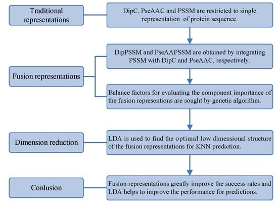
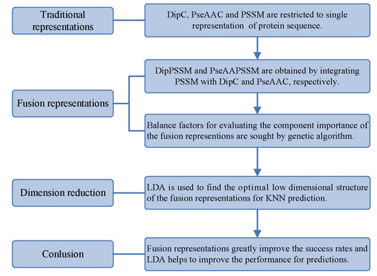
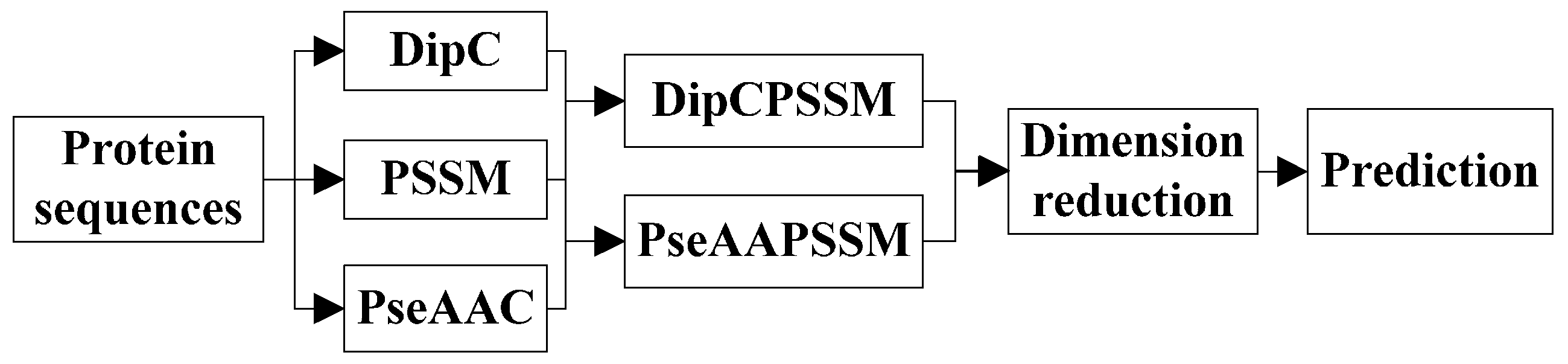
k-nearest neighbors classifier (KNN). In the first process, we specifically take account into both DipC and PSSM to form a new representation, dubbed DipPSSM and consider both PseAAC and PSSM to construct another proposed representation, called PseAAPSSM. In this way, the two proposed representations contain more protein sequence information, and can be sufficient for describing protein data. However, it is difficult to reach a suitable trade-off of DipC and PSSM in DipPSSM and a suitable trade-off of PseAAC and PSSM in PseAAPSSM, so we adopt genetic algorithm to figure out a set of balance factors to solve this problem.
Table 1.
The corresponding relationship between abbreviation and full name.
Table 1.
The corresponding relationship between abbreviation and full name.
| Code | The Full Name | Abbrevition |
|---|
| 1 | Dipeptide composition | DipC |
| 2 | Pseudo-amino acid composition | PseAAC |
| 3 | Position specific scoring matrix | PSSM |
| 4 | The proposed representation by fusing DipC and PSSM | DipPSSM |
| 5 | The proposed representation by fusing PseAAC and PSSM | PseAAPSSM |
| 6 | Linear discriminate analysis | LDA |
| 7 | k-nearest neighbors | KNN |
| 8 | True positive | TP |
| 9 | True negative | TN |
| 10 | False positive | FP |
| 11 | False negative | FN |
| 12 | Mathew’s correlation coefficient | MCC |
In
Section 2, we review three single representations, DIPC, PseAAC and PSSM. In
Section 3, we propose two representations and use genetic algorithm to get the balance factors of the proposed representations. In
Section 4, we perform LDA on the proposed representations followed by KNN classification algorithm. In
Section 5, experiments with two benchmark datasets are performed.
Section 6 gives the concluding remarks. For convenience of the readers, we give a list of all abbreviations of this paper in
Table 1.
3. Two Fusion Representations, DipPSSM and PseAAPSSM, and the Optimization Algorithm
In this section, two fusion representations are introduced and then genetic algorithm is used to seek out the optimal weight coefficients in the fusing process.
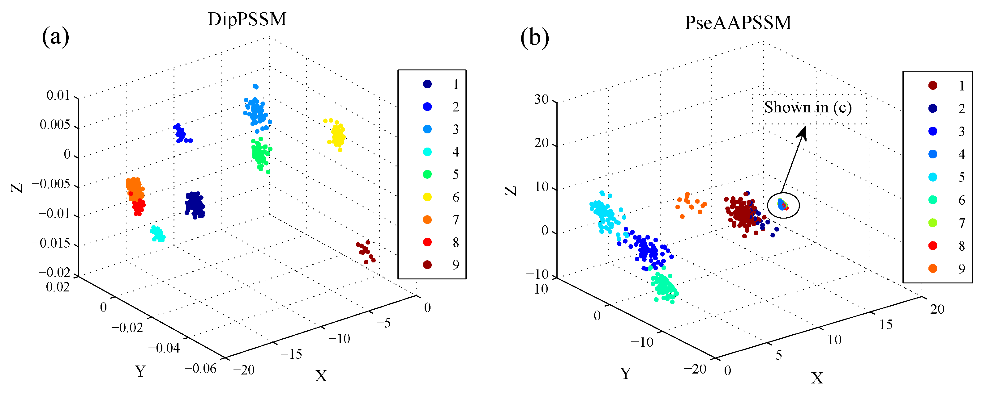
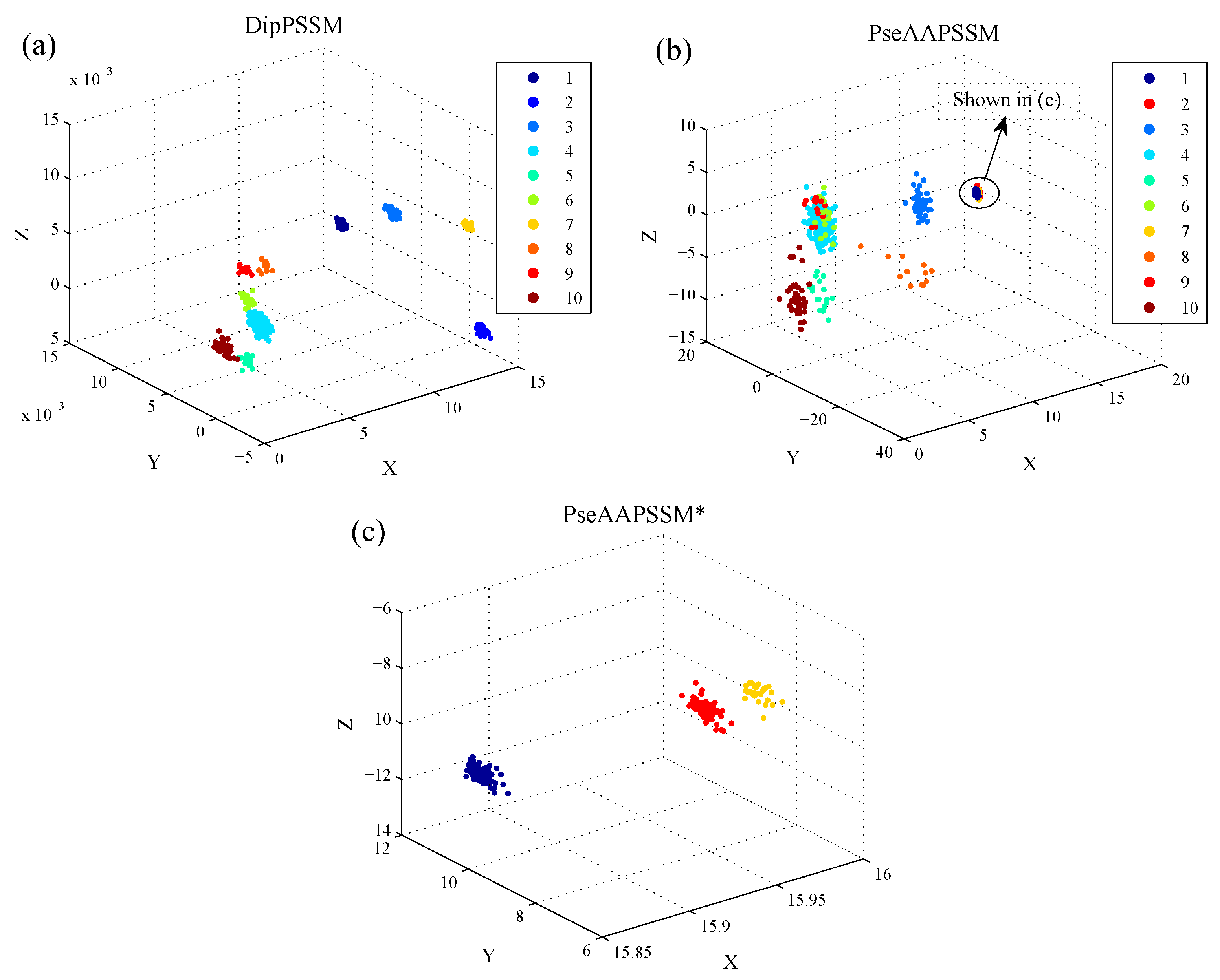
3.1. Two Fusion Representations DipPSSM and PseAAPSSM
Although both of DipC and PseAAC contain the information of the amino acid composition and the sequence order, they reflect different essential features of protein samples. On the other hand, PSSM represents a protein’s evolution information, which DipC and PseAAC do not possess. To this end, we combine PSSM with DipC and PseAAC to form two new representations, called DipPSSM and PseAAPSSM, respectively. Both DipPSSM and PseAAPSSM contain much more protein information than their component representations. Specifically, DipPSSM includes amino acids composition information, amino acids sequence order information and evolutionary information. PseAAPSSM contains amino acids composition information, amino acids sequence order information, the chemical and physical properties of amino acids and evolutionary information.
Now, we introduce the detailed combination of generating the fusion representations, DipPSSM and PseAAPSSM. Suppose that we have a dataset of
N proteins belonging to
n sub-nuclear locations. First, we transform the protein sequence of the
i-th sub-nuclear location into two representations
Ai and
Bi,
i = 1,2,…,
n, where
Ai means DipC or PseAAC and
Bi means PSSM.
Ai and
Bi contain different context information leading to their different effects on protein sub-nuclear localization. Denote
A and
B as follows [
7,
15,
24].
Then, we employ the weight coefficients vector
R to balance the two representations, which is an important idea for combining representations. The mathematical forms of
R can be written as follow:
where
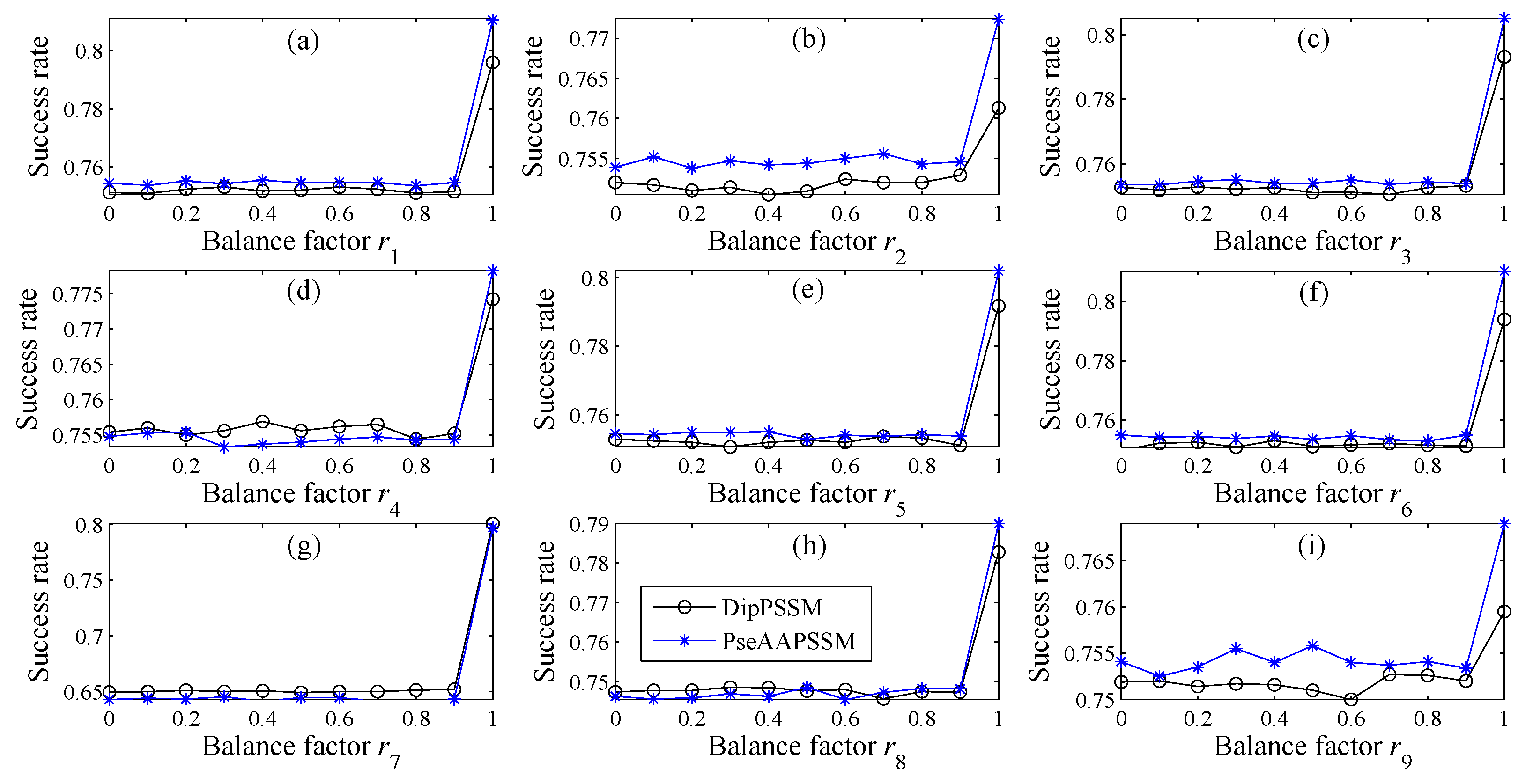
ri (0,1) (
i = 1,2,…,
n) are used to represent the importance of the two representations in each sub-nuclear location, here also called the balance factors. We present the final form of the fusion representation in Equation (9).
In many current literatures, different components of a fusion representation are considered equally important, which is actually a special case of Equation (9) when ri = 0.5 (i = 1,2,…, n). Since the fused representation Equation (9) uses the characteristics of the two single representations reasonably, it contains more protein sequences information and reflects the influence degree of the two single representations. Note that the balance factors for different sub-nuclear locations are not all the same. Besides, since different sub-nuclear locations are an organic whole in the cellular nucleus, the sub-nuclear proteins are interacting with each other, it is proper to think that n balance factors, ri (i = 1,2,…, n), are correlated with each other. Therefore, it is a complex work to select an optimum value of R. In the next subsection, we will discuss how to give a proper value of R.
3.2. Genetic Algorithm—The Optimization Algorithm
Genetic algorithm is an algorithm that imitates the evolution process of biological organism in the nature as an adaptive method that can be used to solve searching and optimizing problems [
26], especially combination optimization problems with high computational complexity, which traditional methods cannot cope with [
27]. In this paper, we employ genetic algorithm to seek out the balance factors
ri (
i = 1,2,…,
n) of the proposed representations. The seeking procedure is as follows.
The first and generally the most difficult step of the genetic algorithm is to create an initial population, which is a pre-determined amount of individuals encoded to map the problem solution into a genetic string, or chromosome [
28]. In genetic algorithm, all the individuals, in term of the coding method and principle, possess the same structure maintaining the genetic information on individuals of population. The second step is to conduct selection, crossover, mutation and replacement depending on the fitness error, under the constraints of the individual population. The final step is to stop iteration when stopping criteria is met.
In this paper, we put forward an initial-population selection strategy to greedily produce initial population. Its detailed process is as follows.
- (1)
Generate a random permutation of the integers traversing from 1 to n (n is the number of sub-nuclear locations), which is the tuning order of the balance vector R.
- (2)
Set 0.5 as the initial value for all elements in R.
- (3)
For each ri, we search from 0 to 1 with 0.01 steps to get the value obtaining the highest prediction accuracy.
- (4)
Repeat step (3) for all the elements of R according to the order in step (1).
- (5)
Repeat step (1–4) 50 times to get 50 sets of balance vectors R. We save these balance vectors as the initial population.
Note that in Step (5), due to the unstable of genetic algorithm, we here run this experiment multiple times to select the optimal solution as the final balance factors. Specifically, we repeat 50 times to generate an initial population. In theory, the greater the number of repetitions, the better the result becomes. Practically, the results trend to be stable when the repetition exceeds 50 times. Therefore, we set a relative reasonable number of 50 due to the cost of computation. After the steps for creating the initial population, we calculate the balance factors via minimizing the fitness error for predicting the sub-nuclear localization. We implement the computation by using MATLAB to work out the balance factors ri (i = 1,2,…, n) delivering by the minimum fitness error.
6. Conclusions
Following the completion of the Human Genome Project, bioscience has stepped into the era of the genome and proteome [
40,
41,
42,
43,
44]. A large amount of computational methods have been presented to deal with the prediction tasks in bioscience [
45,
46,
47,
48]. The nucleus is highly organized and the largest organelle in the eukaryotic cells. Hence, managing protein sub-nuclear localization is important for mastering biological functions of the nucleus. Many current studies discuss protein sub-nuclear localization prediction [
49,
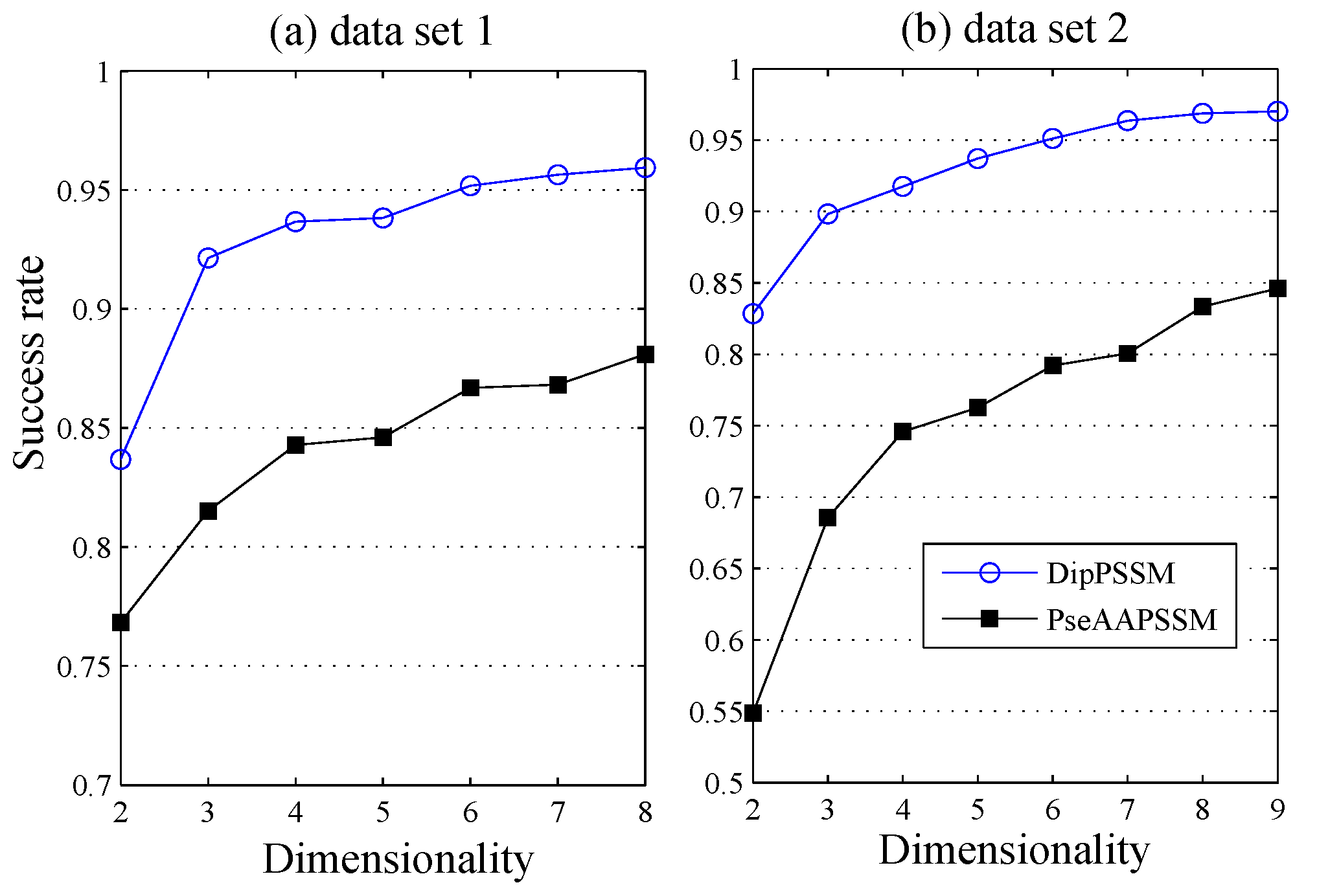
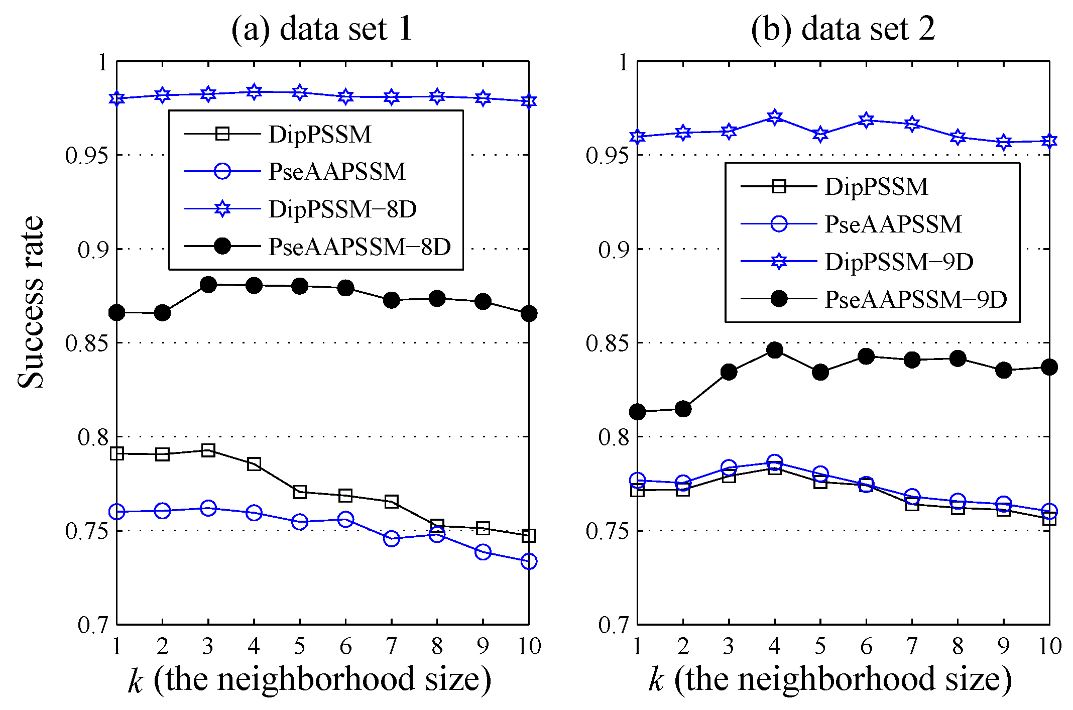
50]. This paper proposes a different route to identify the protein sub-nuclear localization by firstly developing two fusion representations, DipPSSM and PseAAPSSM. Then, we conduct the experiments based on the 10-fold cross validation on two datasets to certify the superiority of the proposed representations and the applicability for predicting protein sub-nuclear localization. Through the present study, we have drawn the conclusions that our fusion representations can greatly improve the success rate in predicting protein sub-nuclear localization, thereby the fusion representations can reflect more overall sequence pattern of a protein than the single one.
However, there is the difficulty of choosing proper balance factors in constructing the fusion representations. The processing method of this paper is to use genetic algorithm to produce approximate optimal values of the weight coefficients (balance factors), where we run the genetic algorithm multiple times to compute the average weight coefficient giving rise to the ideal performance. However, the time complexity of this method is high, so in the future research we will try multiple searching methods for achieving the weight coefficients.
Due to the fact that our proposed fusion representations have high dimensionality, which might result in some negative effects for KNN prediction, we employ LDA to process the representations before using KNN classifier predicts protein locations. Note that, in current pattern recognition research, many other useful data reduction methods such as kernel discriminant analysis and fuzzy LDA have emerged. How to effectively use these methods or their improved methods or other more suitable dimension reducing methods in the sub-nuclear localization field is still an open problem. In addition, it remains an interesting challenge to obtain better representations for protein sub-nuclear localization and study other machine learning classification algorithms.


