Workers’ Exposure to Nano-Objects with Different Dimensionalities in R&D Laboratories: Measurement Strategy and Field Studies

 ,
, 
Abstract
:
1. Introduction
- (1)
- Far-Field (FF) approach: background is measured in a place not influenced by the process, in the same facility, but far from the workplace where NMs are produced. Some authors also consider the FF background measurements as a “spatial approach”, in which the difference between the background and workplace concentrations can be attributed to the work with the NOAA investigated. FF background measurements should be collected simultaneously with the NOAA measurements [15].
- (2)
- Near-Field (NF) approach: based on monitoring before work, at the same location as the nano-workstation. The NF background is also defined as a “time-series” approach, assuming that the concentration determined when there is no ongoing work is the background concentration and any increases during work can be attributed to the process.
2. Results
2.1. Information Gathering (Tier 1)
2.2. Basic Exposure Assessment (Tier 2)
- -
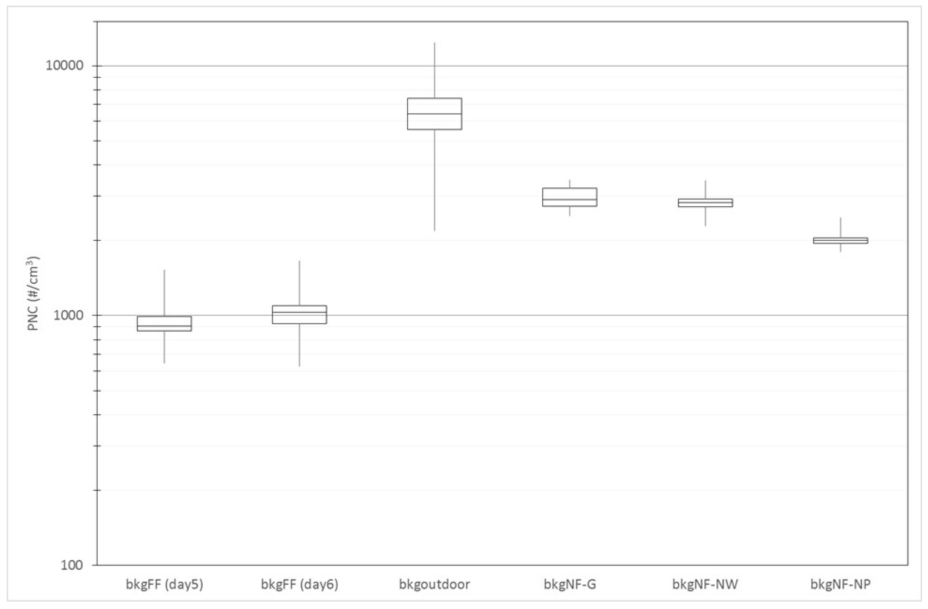
- on day 5 the median, at 907 #/cm3, was much closer to the lower edge whereas on day 6 the median, at 1029 #/cm3, was closer to the upper edge of the box;
- -
- the distribution dispersions (interquartile distance on day 5 was 123 #/cm3 and on day 6 it was 164 #/cm3) were not dissimilar.
3. Discussion
4. Materials and Process Descriptions
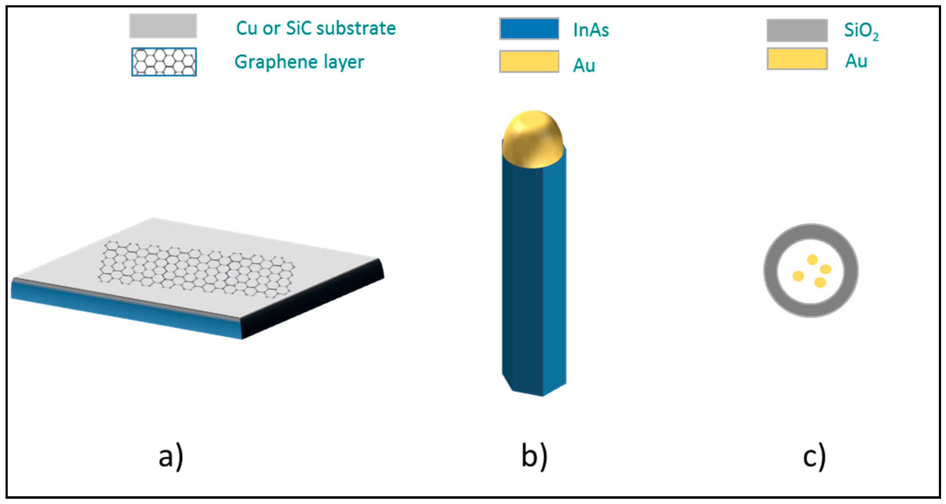
4.1. 2D Graphene (G)
- Sample preparation and loading. The reactor chamber is vented and the reactor lid is lifted manually; the sample (up to 10 × 10 mm) is placed on the graphite heater inside the reactor; the chamber is closed and pumped up to 5 × 10⁻¹ mbar before starting a process.
- CVD Growth. The growth process can be divided into two steps, both conducted in a commercial resistively heated cold-wall reactor (Aixtron HT-BM):
- 2.1.
- Hydrogen etching. SiC substrates are treated with hydrogen etching at a temperature of around 1200 °C and a pressure of 450 mbar for a few minutes, in order to remove polishing scratches and obtain atomically flat terraces.
- 2.2.
- Thermal decomposition. The hydrogen etched substrates are heated in an argon atmosphere at a temperature above 1300 °C and a pressure of 780 mbar for 10–15 min.
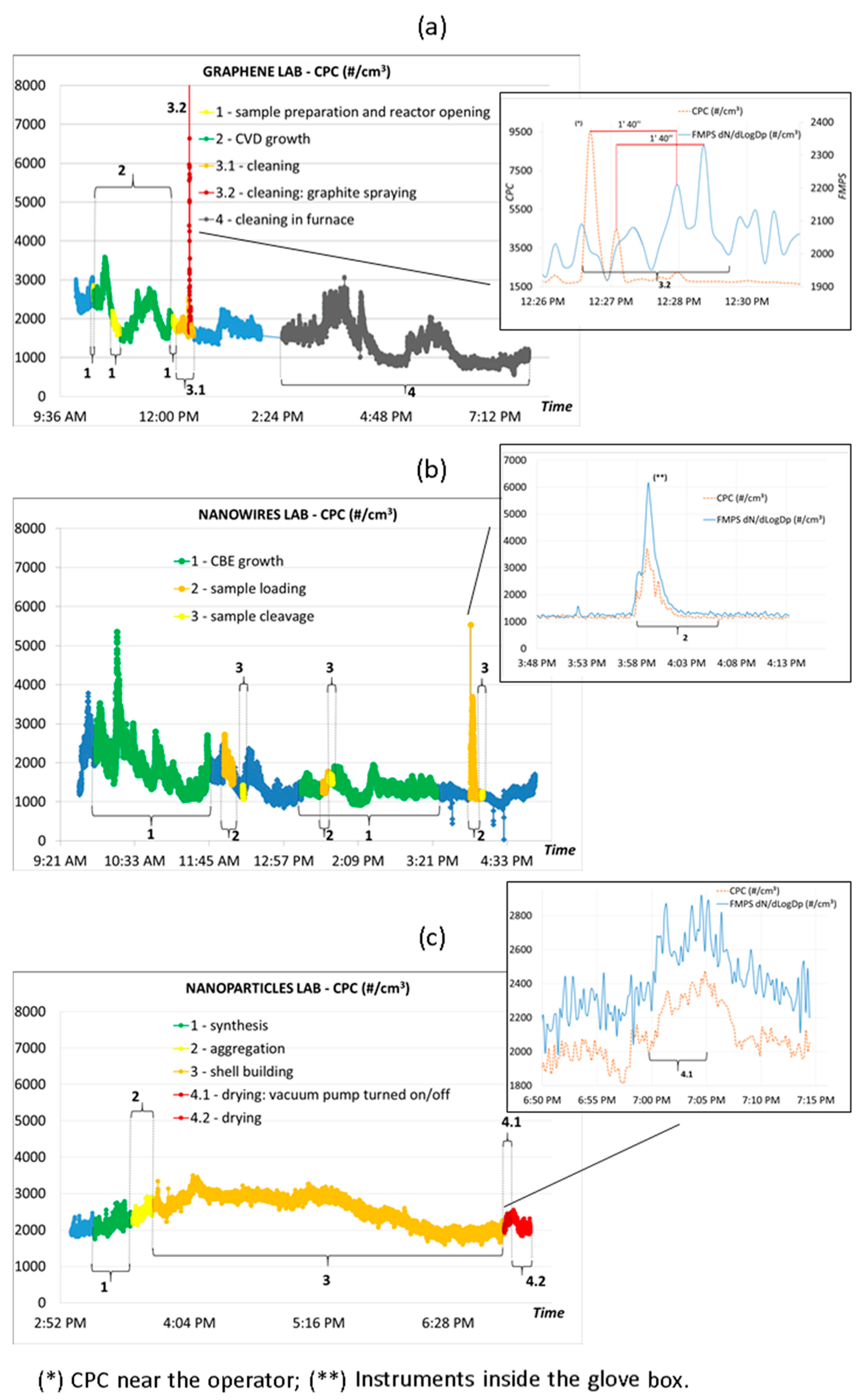
- Reactor cleaning. The quartz and ceramic parts are periodically cleaned in an oven operated in air, in order to remove any carbon deposit. During the cleaning some reactor components are restored by graphite spraying.
- Cleaning in the furnace. The parts are heated at 950 °C for at least one hour.
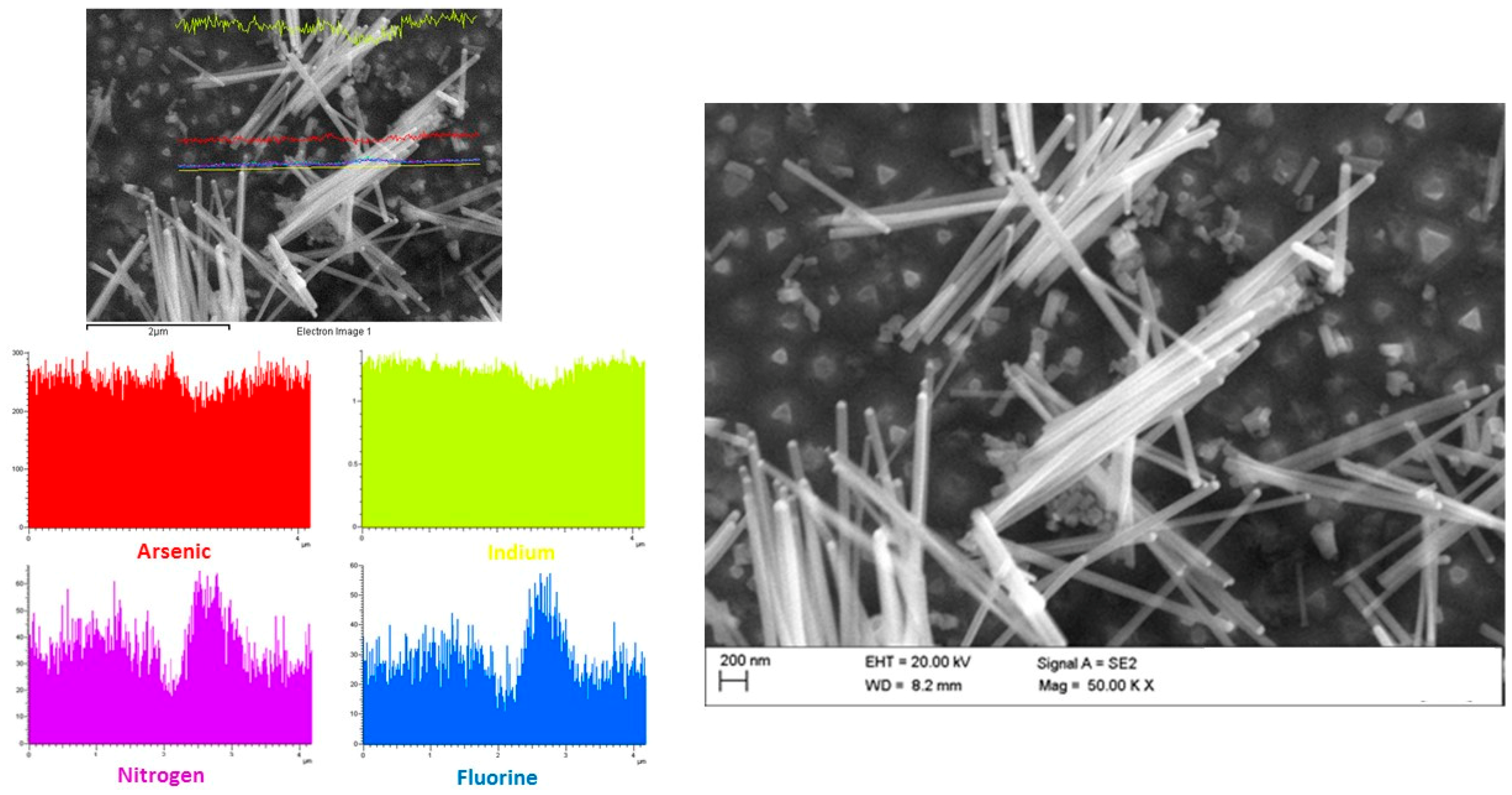
4.2. 1D Nanowires (NW)
- CBE growth. NW are synthesized through epitaxial growth techniques, e.g., the CBE, on a macroscopic crystalline substrate made of a semiconductor material, Si or InAs [30]. Usually, one end of the nanowire (the one not attached to the substrate) is composed of an Au metallic nanoparticle, as a semi-sphere with the same diameter as the NW, employed as catalyst during the growth process. The pressure achieved in the growth chamber is around 10−10 Torr.
- Sample loading. This phase is divided into two following steps:
- 2.1.
- Sample mounting and loading (before CBE growth). The substrate is first cleaved into small pieces of about 1 cm × 1 cm, and then fixed on a sample holder made of Mo through In-bonding inside a glove box. After that, the sample holder is placed in a cassette and transferred into the CBE system via a load-lock. The load-lock is pumped by a turbo-molecular pump and a base pressure of 10−8 Torr can be achieved in 1–2 h. The cassette is then transferred into the preparation chamber, and after that to the growth chamber, for NW synthesis.
- 2.2.
- Sample unloading and unmounting (after the CBE growth). The plates with the grown samples are transferred from the growth chamber into the preparation chamber, mounted on the cassette that is transferred into the load-lock, and then again into the glove box, where the sample holder is placed on a hot plate at about 350 °C, to allow the In to melt, and the sample can be removed from the Mo plate. Frequently, a new sample mounting and loading (phase 2.1) is done immediately after the sample removal (phase 2.2).
- Sample cleavage. The next phase is cleavage of the sample, for its morphological characterization by SEM.
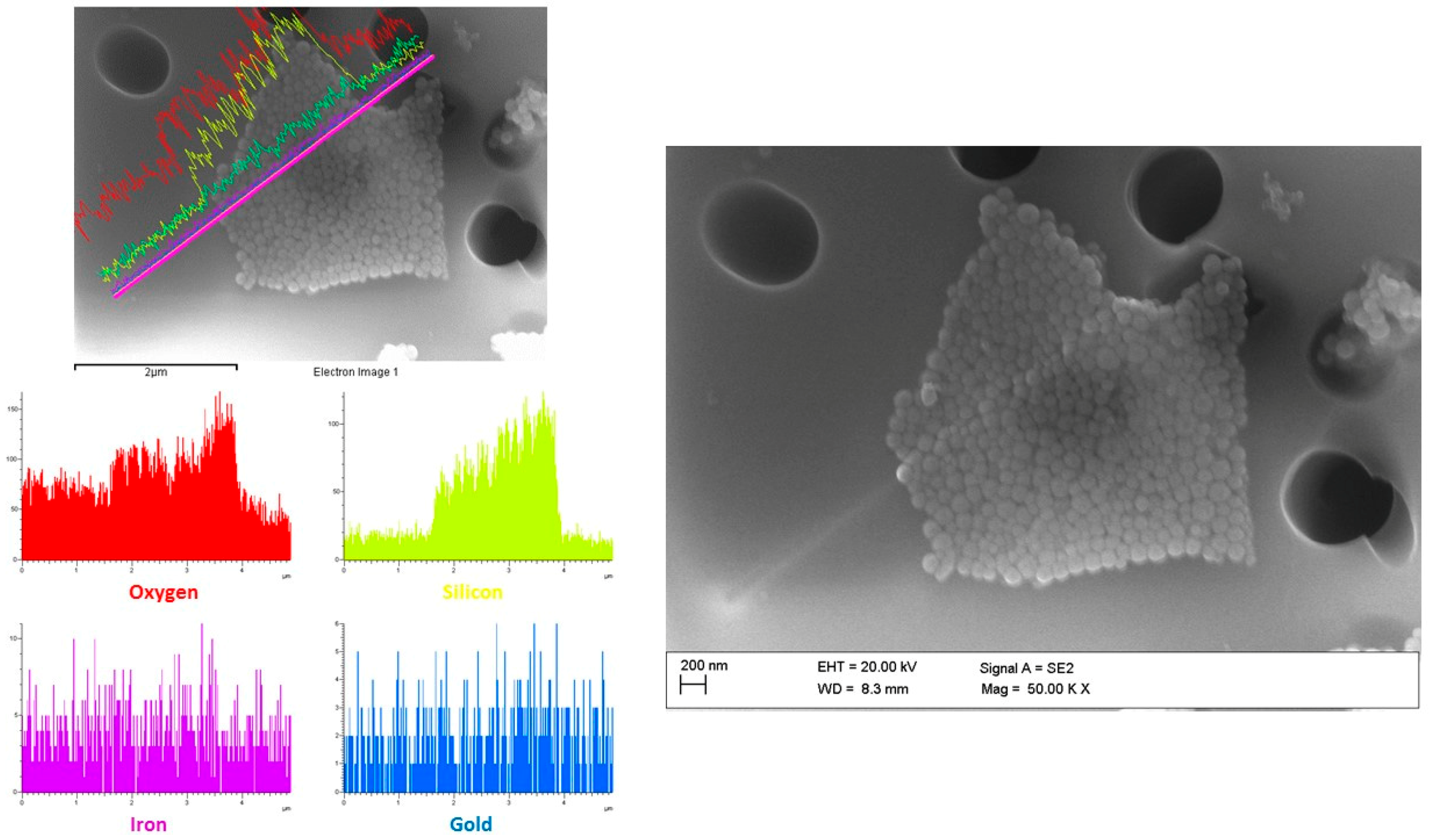
4.3. 0D Nanoparticles (NP)
- Synthesis. The nano-architectures are synthesized by a wet chemical approach. A yellow solution of chloroauric acid underwent fast reduction by sodium borohydride in the presence of poly(sodium 4-styrene sulfonate) (PSS), with vigorous stirring, resulting in a deep orange colloidal solution of negatively charged gold NP, less than 3 nm in diameter.
- Aggregation. The 3 nm gold NP are then assembled in spherical arrays by controlled aggregation achieved by ionic interaction with positive poly(l-lysine) (PL).
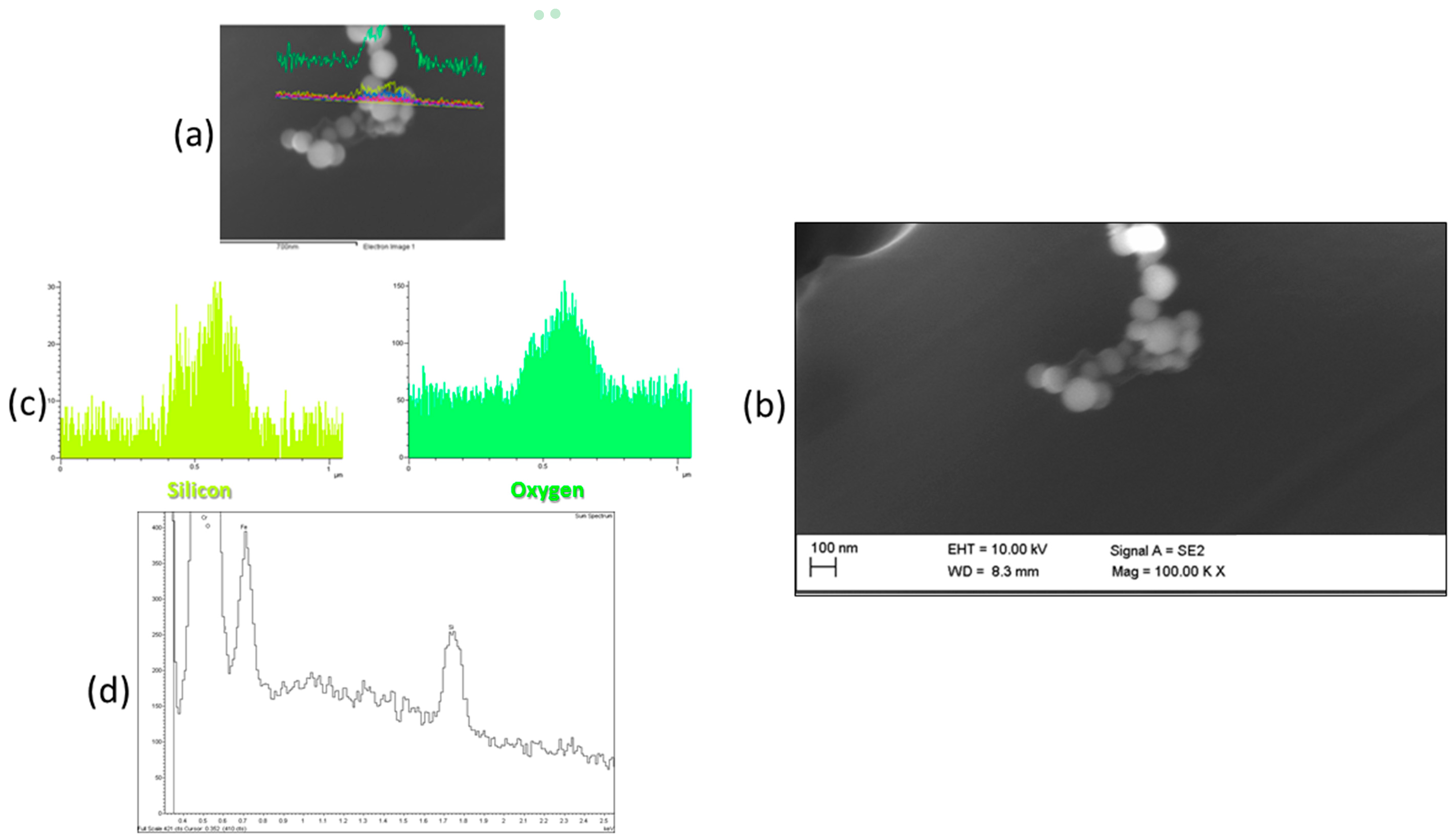
- Shell building. The arrays are purified by cycles of centrifugation and silica-coated by a modified Stöber method [34]. The resulting products are “passion fruit-like” nano-architectures averaging 100 nm in diameter, with 20 nm wall thickness, and containing 1–10% w/w of metal.
- Drying. The colloidal solutions were usually frozen in liquid nitrogen and freeze-dried overnight to obtain a red powder (about 1 mg for each synthesis with an estimated total laboratory production of 1 g/year).
5. Methods
- Condensation particle counter (CPC mod. 3007, TSI Inc., Shoreview, MN, USA) to measure in real-time the number concentration (#/cm3) of particles from 10 nm to 1 µm, with 1 s time resolution and accuracy ±20%; (total flow 0.7 L/min; detection limits 1 to 100,000 #/cm3).
- Personal samplers (mod. Sioutas, SKC Inc., Eighty Four, PA, USA) equipped with a pump (mod. Leland Legacy, SKC Inc., 9 L/min flow) for concentrations (#/cm3) of particles from 250 nm to 2.5 µm (five stages).
- Field emission scanning electron microscope (FE-SEM) Ultra Plus (ZEISS) with EDS probe Inca 250-X-Max50 and INCA mapping software in line scan mode. The microscope is equipped with a modified Gemini column and has four different detectors: in-chamber Everhat–Thornely SE for surface topography, in-column In lens best for high efficiency, angle-selective backscattered detector ASB for material contrast and topographical information, in-column ESB for material contrast even at low KV.
- Microclimatic probes integrated in a control unit (BABUC-A, Lsi-Lastem Inc., Milano, Italy) to measure in real time physical parameters such as temperature, RH and air speed.
- Fast mobility particle sizer (FMPS mod. 3550, TSI Inc.) to characterize real-time size distribution and simultaneously measure total particle numbers and mass concentration, in the size interval 5.6–560 nm, with 1 s time resolution;
- Nanoparticle surface area monitor (NSAM mod. 3091, TSI Inc.) to measure average and cumulative surface area (µm2/cm3) of particles from 10 nm to 1 µm, with 1 s time resolution, corresponding to the tracheobronchial (TB) or alveolar (A) pulmonary fractions, based on the model published by the International Commission on Radiological Protection [35];
- PAS 2000 (EcoChem Analytics, League City, TX USA) to measure polycyclic aromatic hydrocarbons (PAHs) surface-adsorbed on carbon aerosol with aerodynamic diameter from 10 nm to 1.5 µm, with a response time of 10 s in a measuring interval from 0 to 1000 ng/m3 and a lower detection limit of 3 ng/m3.
- Ozone analyzer (mod. 49, Thermo Environmental Instruments Inc., Franklin, MA, USA) to measure ozone levels in the air.
- Nano micro orefice uniform deposit impactor (nanoMOUDI-II 122R, MSP Corp., Shoreview, MN, USA), equipped with a rotary pump (BUSH LLC., Virginia Beach, VA, USA, 30 L/min flow), to collect particles in a dimensional range from 10 nm to 10 µm.
- Inductively coupled plasma mass spectrometry (ICP-MS 820, Bruker Corp., Billerica, MA, USA).
- Inductively coupled plasma optical emission spectroscopy (ICP-OES Agilent 5100, Agilent Technologies, Santa Clara, CA, USA).
- Atomic fluorescence spectrometer (AFS Titan 8200, Beijing Titan Instruments Co., Beijing, China).
6. Conclusions
- -
- G laboratory. Real-time measurements showed high PNC associated with phase 3.2 of graphite spraying during the CVD reactor cleaning, but SEM did not detect any produced G on the sampled filters. As a precautionary measure, this specific phase should be conducted under an aspiration hood or in a glove box.
- -
- NW laboratory. Although the CPC measurements showed a rise in PNC during phase 2 (sample mounting and loading/unloading and unmounting), SEM did not detect any NW on the Sioutas filters. Although the PNC was probably related to sublimation of In from the hot Mo plate, an ad hoc investigation is called for to properly analyze the chemical and physical parameters of the emission source in this specific phase. In any case, the measurements made inside the glove box demonstrated the effectiveness of this containment measure. The study of the CBE reactor cleaning phase (not included in the present measurement campaign), might be useful to analyze the whole process so as to finally exclude workers’ exposure to NW.
- -
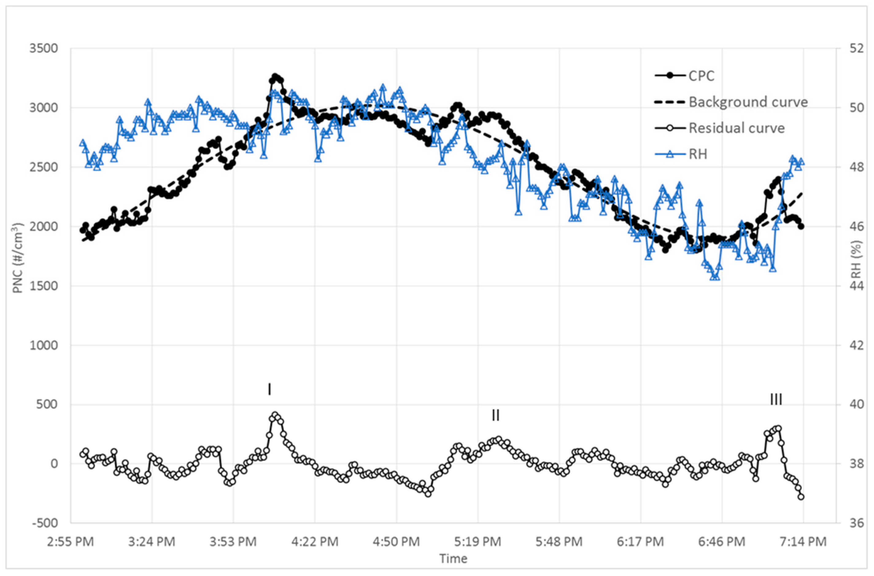
- NP laboratory. In a large part of the process, PNCs were greater than the significant value identified for this laboratory. In this case the background contribution heavily influenced the PNC, as measured by CPC, so we proposed a different type of analysis to take account of the background. By comparison of CPC time series with microclimatic parameters measured with BABUC-A probes, with particular reference to the RH throughout the sampling period, we found a structure corresponding to phase 4.1 (drying vacuum pump turned on) that exceeded the background curve; the PNC increase in this case is probably related to the pump switching and not strictly connected to NP production. However, SEM of sampled filters showed there were rare spherical SiO2 particles (with an approximate diameter of 100 nm) similar to the hollow silica shells produced but with no evidence of the Au nanostructures inside. This implies that further investigation is needed to confirm whether such NPs are in fact released by the process and in which specific phase this release might occur.
Acknowledgments
Author Contributions
Conflicts of Interest
Appendix A

| Technical Data Sheets | NP | NW | G |
|---|---|---|---|
| 1. NOAA information | |||
| 1.1 Technical name and/or commercial name | Hollow silica nanoparticles with embedded gold nanoparticles (AuSiO2) | Semiconductor nanowires (NW) | Graphene |
| 1.2 CAS Number | CAS number Au: 7440-57-5 CAS number SiO2: 7631-86-9 CAS number Poly-l-lysine hydrobromide 15–30 kDa: 25988-63-0 CAS number Poly(sodium 4-styrenesulfonate) 70 kDa: 25704-18-1 | n.a. (CAS number InAs) | n.a. (CAS number Carbon) |
| 1.3 Molecular structure/Crystal structure | 100 nm silica (SiO2) nanocapsules containing: (i) 30–500 gold nanoparticles with diameters 2–4 nm; (ii) poly(l-lysine) 15–30 kDa; (iii) poly(sodium 4-styrenesulfonate) 70 kDa | Crystal structure: mainly hexagonal (Wurzite) with cubic insertions (Zincoblende). NW have their long axis oriented along the hexagonal c-axis which is parallel to the cubic <111> direction | Single atomic layer of carbon atoms disposed in a honeycomb lattice |
| 1.4 Chemical composition (including surface compounds) | The powders are 5% gold and 95% silica (SiO2) and organic polymers. | InAs (50/50) with a top Au0.5In0.5 nanoparticle (eutectic). | Carbon |
| 1.5 Physical form and shape | Spherical nanoparticles | NW are rod-shaped crystals, with hexagonal cross-section and a AuIn nanoparticle attached at one end. | Bi-dimensional crystal taking the form of flakes |
| 1.5.1 Common form | The common forms are: (i) powder (after freeze-drying) (ii) in water solutions | NW grow normal to the InAs (111) substrate surface, forming a “forest” connected to the substrate at one end. | Single crystals with dimensions from microns to millimeters |
| 1.6 Surface chemistry | Negative charge (−21 V in PBS) | InAs | Carbon |
| 1.7 Production method | Wet chemical synthesis | Chemical Beam Epitaxy (CBE) synthesis | Chemical Vapor Deposition (CVD) synthesis |
| 2. NOAA Characterization | |||
| 2.1 Aggregation/Agglomeration | Single nanoparticles in solutions. Possible aggregation after freeze-drying | NW can agglomerate if detached from the substrate | If detached from the substrate they can aggregate |
| 2.2 Solubility | Tested, up to 100 mg/mL in aqueous solutions | Insoluble in bases, organic solvents and biological media. Soluble in acids. | Non soluble |
| 2.2.1 Dispersibility | Up to 100 mg/mL in ethanol | NW can be dispersed in liquid (i.e., 2-propanol) via sonication or by mechanical transfer from the substrate. | Can be dispersed in organic solvents |
| 2.3 Crystal phase | n.a. | NW are single crystals with a lattice parameter of 6.0583 Angstrom | Hexagonal bi-dimensional lattice |
| 2.4 Dustiness (or bulk material density) | n.a. | Bulk InAs density: 5.67 g/cm3 | n.a. |
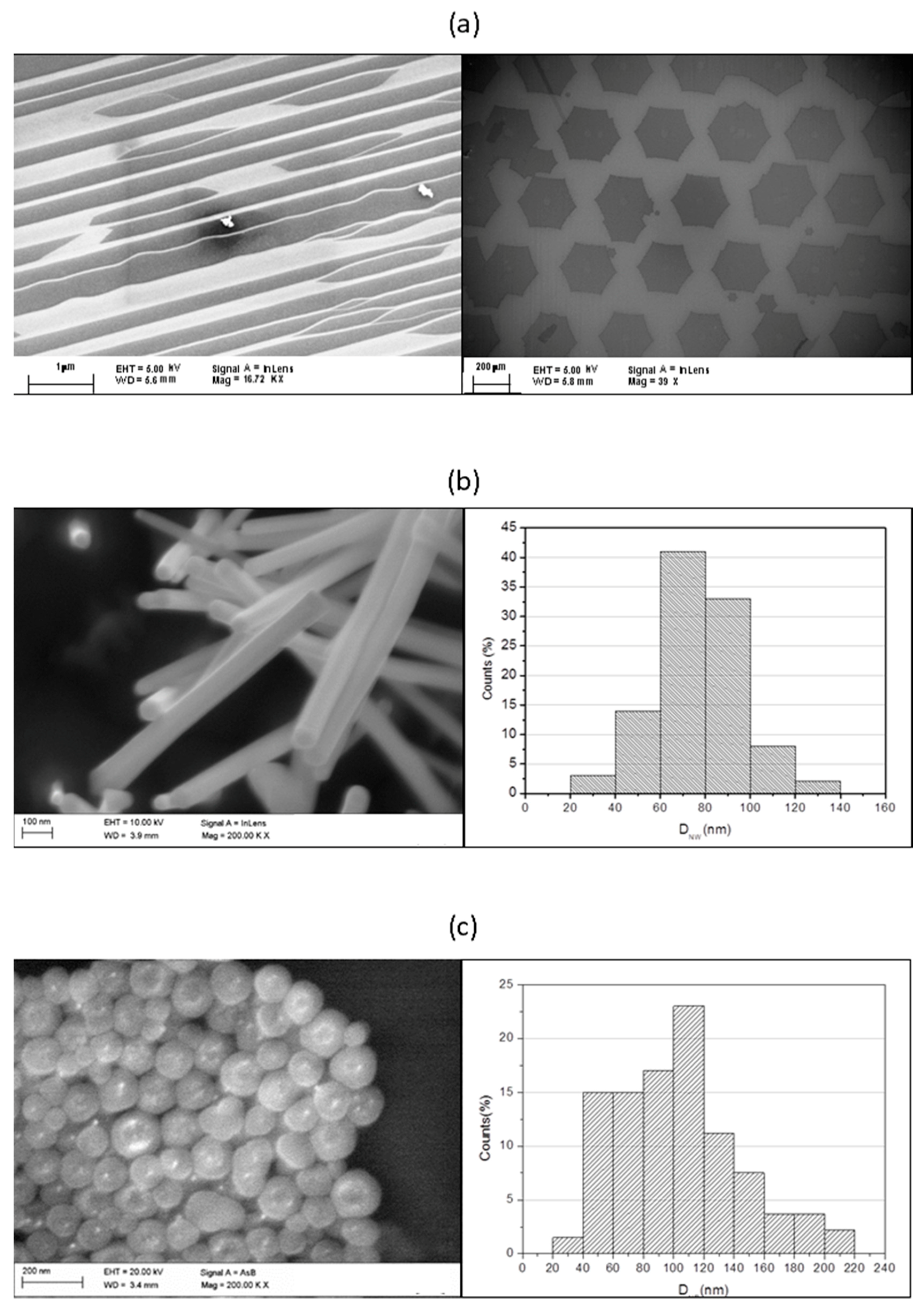
| 2.5 Representative image (SEM) | See attached Figure A1 | See attached Figure A2 | In Convertino et al. [36] |
| 2.6 Size | 100 ± 20 from TEM images (analysis of at least 300 nanoparticles) | NW can be synthetized with average diameters in the 30–100 nm range, and lengths of 1–2 μm. Dimensions are typically obtained from SEM images. | Graphene flakes have lateral dimensions that vary from fraction of microns to millimeters |
| 2.7 Surface area | About 30,000 nm2/nanostructure | 300,000 nm2 (1 NW) | n.a. |
| 2.8 Catalytic or photocatalytic activity | No | No | n.a. |
| 2.9 Density | n.a. | Average substrate area density of NW ranges from 1 to 250 NW per μm2. Area density is determined from SEM images. If left attached to the substrate the area density is indicated as above. Concerning the “mass per unit volume” density of the NW layer on the substrate surface (considering “typical” 60 nm in diameter and 1 μm length NW with an area density of 50 NW/μm2): it is a 1 μm thick layer covering the whole substrate surface with normal-to-the-substrate NW. This layer has an average density of 0.8 g/cm3 | n.a. |
| 2.10 Porosity | n.a. | No | n.a. |
| 2.11 Surface reactivity | Covalent bonding with silanols (ex. APTES). Possible adsorptions of positive molecules | Little reactivity | n.a. |
| 2.12 Other information | n.a. | n.a. | n.a. |
| 3. Processes | |||
| 3.1 Average quantity produced/used per year | 1 g | 20 mg | 2–3 mg |
| 3.2 Average quantity produced/used in each process | 1 mg | 40 μg | 1 µg |
| 3.3 Process phases description |
|
|
|
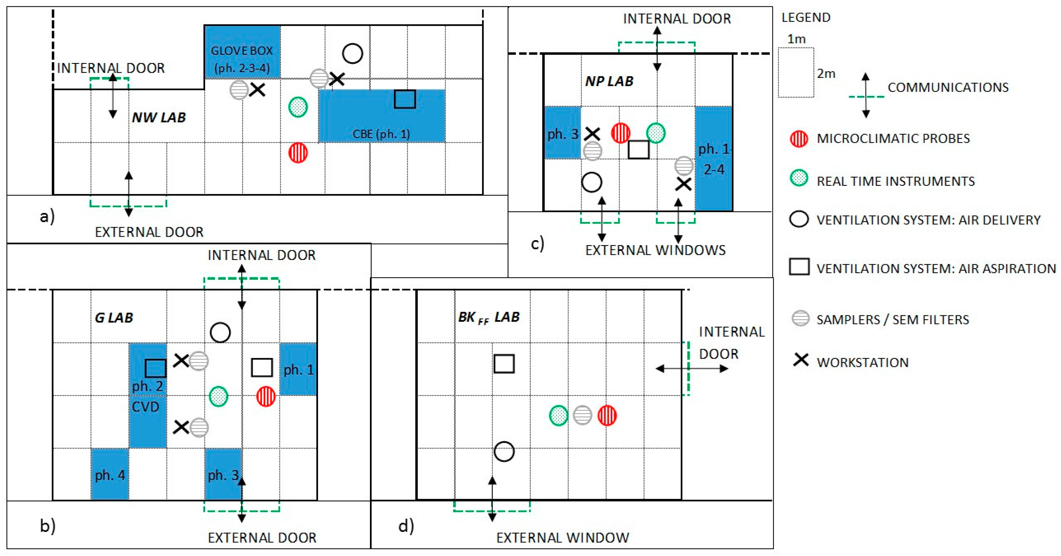
| 3.4 Workplace description | The NP laboratory has an area of 30 m2 (about 90 m3 of volume) | The NW laboratory has an area of 20 m2 (about 60 m3 of volume) | G laboratory has an area of 40 m2 (about 120 m3 of volume) |
| 3.4.1 Other processes in the same workplace | The synthesis are performed in the lab where are also performed chemical synthesis and purifications of organic molecules. | Substrates with NW can be cleaved inside the negative pressure glove box to do SEM observation or other characterization. During SEM observation (taking place in an ISO6 cleanroom) o additional processes take place. | n.a. |
| 3.4.2 Ventilation system | Mechanical ventilation system producing an air change of 3 volumes per hour | Mechanical ventilation system producing an air change of 3 volumes per hour; in case of emergency an automatic system for aspiration/cleaning starts. | Mechanical ventilation system producing an air change of 3–6 volumes per hour |
| 3.5 Number of workers | 1 | 2–3 | 1–2 |
| 3.7 Avg duration of production process | 5 h | 2 h | 2 days |
| 3.8 Avg working days per year | 250 | 230 | n.a. |
| 3.9 Number of production processes per day | 0–6 | 3–4 | n.a. |
| 3.10 Risk assessment method and results | Control Banding: Medium | Control Banding: High | Control Banding: High |
| 3.11 Exposure measurements/monitoring | n.a. | n.a. | n.a. |
| 3.12 Safety operating procedures | yes | yes | yes |
| 3.13 Protective equipment | Phases 1 and 4 are performed within chemical ventilated hood. Worker equipped with personal protective devices (gloves, clothing and glasses). | Phase 1 is in closed system (ultra-high-vacuum reactor); phases 2–3 are performed in a ventilated glove box. Workers are equipped with personal protective devices (gloves, clothing, half- and full-face masks with A2B2E2K2P3 filters). | Phases 2 and 4 are fulfilled in a closed system. Workers are equipped with personal protective devices (gloves, clothing and masks). |
| 4. References | |||
| 4.1 Main references | Voliani and Piazza [37], Cassano et al. [38] | Tomioka et al. [39], Gomes et al. [30], Rocci et al. [40]. | Novoselov et al. [41], Convertino et al. [36], Miseikis et al. [42] |
| 5. Other | |||
| 5.1 Any other available information | n.a. | n.a. | n.a. |


References
- United Nations Educational Scientific and Cultural Organization (UNESCO). Science Report: Towards 2030; UNESCO: Paris, France, 2015; ISBN 978-92-3-100129-1. Available online: http://en.unesco.org/unesco_science_report (accessed on 21 August 2017).
- The ObservatoryNano Project. European Nanotechnology Landscape Report; ObservatoryNANO Work Package 3; European Commission: Brussels, Belgium, 2012; Available online: http://www.nanotec.it/public/wp-content/uploads/2014/04/ObservatoryNano_European_Nanotechnology_Landscape_Report.pdf (accessed on 21 August 2017).
- Vance, M.E.; Kuiken, T.; Vejerano, E.P.; McGinnis, S.P.; Hochella, M.F., Jr.; Rejeski, D.; Hull, M.S. Nanotechnology in the real world: Redeveloping the nanomaterial consumer products inventory. Beilstein J. Nanotechnol. 2015, 6, 1769–1780. [Google Scholar] [CrossRef] [PubMed]
- European Parliament. Horizon 2020: Key Enabling Technologies (KETs), Booster for European Leadership in the Manufacturing Sector. Directorate General for Internal Policies Policy Department A: Economic and Scientific Policy; IP/A/ITRE/2013-01. October 2014. Available online: http://www.europarl.europa.eu/RegData/etudes/STUD/2014/536282/IPOL_STU(2014)536282_EN.pdf (accessed on 21 August 2017).
- International Organization for Standardization (ISO). Nanotechnology—Vocabulary—Part 4: Nanostructured Materials; ISO-TS 80004-4: 2011; International Organization for Standardization: Geneva, Switzerland, 2011. [Google Scholar]
- Maynard, A.D.; Aitken, R.J. ‘Safe handling of nanotechnology’ ten years on. Nat. Nanotechnol. 2016, 11, 998–1000. [Google Scholar] [CrossRef] [PubMed]
- Schulte, P.A.; Geraci, C.L.; Murashov, V.; Kuempel, E.D.; Zumwalde, R.D.; Castranova, V.; Hoover, M.D.; Hodson, L.; Martinez, K.F. Occupational safety and health criteria for responsible development of nanotechnology. J. Nanopart. Res. 2014, 16, 2153. [Google Scholar] [CrossRef] [PubMed]
- Oberdorster, G.; Oberdorster, E.; Oberdorster, J. Nanotoxicology: An emerging discipline evolving from studies of ultrafine particles. Environ. Health Perspect. 2005, 113, 823–839. [Google Scholar] [CrossRef] [PubMed]
- Maynard, A.D.; Aitken, R.J. Assessing exposure to airborne nanomaterials: Current abilities and future requirements. Nanotoxicology 2007, 1, 26–41. [Google Scholar] [CrossRef]
- Dekkers, S.; Oomen, A.G.; Bleeker, E.A.J.; Vandebriel, R.J.; Micheletti, C.; Cabellos, J.; Janer, G.; Fuentes, N.; Vazquez-Campos, S.; Borges, T.; et al. Towards a nanospecific approach for risk assessment. Reg. Toxicol. Pharmacol. 2016, 80, 46–59. [Google Scholar] [CrossRef] [PubMed]
- Brouwer, D.; van Duuren-Stuurman, B.; Berges, M.; Jankowska, E.; Bard, D.; Mark, D. From workplace air measurement results towards estimates of exposure? Development of a strategy to assess exposure to manufactured nano-objects. J. Nanopart. Res. 2009, 11, 1867–1881. [Google Scholar] [CrossRef]
- Kuhlbusch, T.A.J.; Asbach, C.; Fissan, H.; Göhler, D.; Stintz, M. Nanoparticle exposure at nanotechnology workplaces: A review. Part. Fibre Toxicol. 2011, 8, 22. [Google Scholar] [CrossRef] [PubMed]
- Ding, Y.; Kuhlbusch, T.A.J.; Van Tongeren, M.; Sánchez Jiménez, A.; Tuinman, I.; Chen, R.; Larraza Alvarez, I.; Mikolajczyk, U.; Nickel, C.; Meyer, J.; et al. Airborne engineered nanomaterials in the workplace—A review of release and worker exposure during nanomaterial production and handling processes. J. Hazard. Mater. 2017, 322, 17–28. [Google Scholar] [CrossRef] [PubMed]
- Boccuni, F.; Gagliardi, D.; Ferrante, R.; Rondinone, B.M.; Iavicoli, S. Measurement techniques of exposure to nanomaterials on the workplace for low- and medium-income countries: A systematic review. Int. J. Hyg. Environ. Health 2017, 220, 1089–1097. [Google Scholar] [CrossRef] [PubMed]
- Brouwer, D.H.; Berges, M.; Virji, M.A.; Fransman, W.; Bello, D.; Hodson, L.; Gabriel, S.; Tielemans, E. Harmonization of Measurement Strategies for Exposure to Manufactured Nano-Objects: Report of a Workshop. Ann. Occup. Hyg. 2012, 56, 1–9. [Google Scholar] [CrossRef] [PubMed]
- European Committee for Standardization (CEN). Nanotechnologies—Guidance on Measurands for Characterising Nano-Objects and Materials that Contain Them; CEN/TS 17010:2016; European Committee for Standardization: Brussels, Belgium, 2016. [Google Scholar]
- International Organization for Standardization (ISO). Nanotechnologies—Measurement Technique Matrix for the Characterization of Nano-Objects; ISO/TR 18196:2016; International Organization for Standardization: Geneva, Switzerland, 2016. [Google Scholar]
- Organization for Economic Cooperation and Development (OECD). Harmonized Tiered Approach to Measure and Assess the Potential Exposure to Airborne Emissions of Engineered Nano-Objects and Their Agglomerates and Aggregates at Workplaces. ENV/JM/MONO(2015)19. 17 June 2015. Available online: http://www.oecd.org/officialdocuments/publicdisplaydocumentpdf/?cote=env/jm/mono(2015)19&doclanguage=en (accessed on 21 August 2017).
- Zalk, M.D.; Paik, S.Y.; Swuste, P. Evaluating the Control Banding Nanotool: A qualitative risk assessment method for controlling nanoparticle exposures. J. Nanopart. Res. 2009, 11, 1685–1704. [Google Scholar] [CrossRef]
- Brouwer, D.H. Control Banding Approaches for Nanomaterials. Ann. Occup. Hyg. 2012, 56, 506–514. [Google Scholar] [CrossRef] [PubMed]
- International Standards Organization (ISO). Nanotechnologies—Occupational Risk Management Applied to Engineered Nanomaterials—Part 2: Use of the Control Banding Approach; ISO/TS 12901-2:2014; International Standards Organization: Geneva, Switzerland, 2014. [Google Scholar]
- Iavicoli, I.; Fontana, L.; Pingue, P.; Todea, A.; Asbach, C. Assessment of occupational exposure to engineered nanomaterials in research laboratories using personal monitors and samplers. under review.
- Zhirong, W.; Yuanyuan, H.; Juncheng, J. Numerical investigation of leaking and dispersion of carbon dioxide indoor under ventilation condition. Energy Build. 2013, 66, 461–466. [Google Scholar] [CrossRef]
- Asbach, C.; Kaminski, H.; Fissan, H.; Monz, C.; Dahmann, D.; Mulhopt, S.; Paur, H.S.; Kiesling, H.J.; Herrmann, F.; Voetz, M.; et al. Comparison of four mobility particle sizers with different time resolution for stationary exposure measurements. J. Nanopart. Res. 2009, 11, 1593–1609. [Google Scholar] [CrossRef]
- Brouwer, D.; Boessen, R.; van Duuren-Stuurman, B.; Bard, D.; Moehlmann, C.; Bekker, C.; Fransman, W.; Klein Entink, R. Evaluation of decision rules in a tiered assessment of inhalation exposure to nanomaterials. Ann. Occup. Hyg. 2016, 60, 949–959. [Google Scholar] [CrossRef] [PubMed]
- Fonseca, A.S.; Maragkidou, A.; Viana, M.; Querol, X.; Hämeri, K.; de Francisco, I.; Estepa, C.; Borrell, C.; Lennikov, V.; de la Fuente, G.F. Process-generated nanoparticles from ceramic tile sintering: Emissions, exposure and environmental release. Sci. Total Environ. 2016, 565, 922–932. [Google Scholar] [CrossRef] [PubMed]
- Asbach, C.; Kuhlbusch, T.; Kaminski, H.; Stahlmecke, B.; Plitzko, S.; Götz, U.; Voetz, M.; Kiesling, H.J.; Dahmann, D. NanoGEM Standard Operation Procedures for Assessing Exposure to Nanomaterials, Following a Tiered Approach; Federal Ministry of Education and Research: Heinemannstraße, Germany, 2012. Available online: http://www.nanogem.de/cms/nanogem/upload/Veroeffentlichungen/nanoGEM_SOPs_Tiered_Approach.pdf (accessed on 6 December 2017).
- European Committee for Standardization (CEN). Workplaces Atmosphere Terminology; EN 1540:1998; European Committee for Standardization: Brussels, Belgium, 1998. [Google Scholar]
- Chonan, T.; Taguchi, O.; Omae, K. Interstitial pulmonary disorders in indium-processing workers. Eur. Respir. J. 2007, 29, 317–324. [Google Scholar] [CrossRef] [PubMed]
- Gomes, U.P.; Ercolani, D.; Zannier, V.; Beltram, F.; Sorba, L. Controlling the diameter distribution and density of InAs nanowires grown by Au-assisted methods. Semicond. Sci. Technol. 2015, 30, 010301–014013. [Google Scholar] [CrossRef]
- Olivares, G.; Johansson, C.; Strom, J.; Hansson, H.C. The role of ambient temperature for particle number concentrations in a street canyon. Atmos. Environ. 2007, 41, 2145–2155. [Google Scholar] [CrossRef]
- Morawska, L.; Ristovski, Z.; Jayaratne, E.R.; Keogh, D.U.; Ling, X. Ambient nano and ultrafine particles from motor vehicle emissions: Characteristics, ambient processing and implications on human exposure. Atmos. Environ. 2008, 42, 8113–8138. [Google Scholar] [CrossRef] [Green Version]
- Goldstein, J.; Newbury, D.E.; Joy, D.C.; Lyman, C.E.; Echlin, P.; Lifshin, E.; Sawyer, L.; Michael, J.R. Scanning Electron Microscopy and X-ray Microanalysis, 3rd ed.; Springer: New York, NY, USA, 2003; ISBN 978-1-4615-0215-9. [Google Scholar]
- Stöber, W.; Fink, A.; Bohn, E. Controlled growth of monodisperse silica spheres in the micron size range. J. Colloid Interface Sci. 1968, 26, 62–69. [Google Scholar] [CrossRef]
- International Commission on Radiological Protection (ICRP). Human Respiratory Tract Model for Radiological Protection. Ann. ICRP 1994, 24, 1–482. [Google Scholar]
- Convertino, D.; Rossi, A.; Miseikis, V.; Piazza, V.; Coletti, C. Thermal decomposition and chemical vapor deposition: A comparative study of multi-layer growth of graphene on SiC(000-1). MRS Adv. 2016, 1, 3667–3672. [Google Scholar] [CrossRef]
- Voliani, V.; Piazza, V. Hollow Nanoparticles Having a Modulable Metal Core. International Patent WO2016,139,591, 9 September 2016. [Google Scholar]
- Cassano, D.; Rota Martir, D.; Signore, G.; Piazza, V.; Voliani, V. Biodegradable hollow silica nanospheres containing gold nanoparticle arrays. Chem. Commun. 2015, 51, 9939–9941. [Google Scholar] [CrossRef] [PubMed]
- Tomioka, K.; Yoshimura, M.; Fukui, T. A III–V nanowire channel on silicon for high-performance vertical transistors. Nature 2012, 488, 189–192. [Google Scholar] [CrossRef] [PubMed]
- Rocci, M.; Rossella, F.; Gomes, U.P.; Zannier, V.; Rossi, F.; Ercolani, D.; Sorba, L.; Beltram, F.; Roddaro, S. tunable esaki effect in catalyst-free InAs/GaSb core−shell nanowires. Nano Lett. 2016, 16, 7950–7955. [Google Scholar] [CrossRef] [PubMed]
- Novoselov, K.S.; Geim, A.K.; Morozov, S.V.; Jiang, D.; Zhang, Y.; Dubonos, S.V.; Grigorieva, I.V.; Firsov, A.A. Electric field effect in atomically thin carbon films. Science 2004, 306, 666–669. [Google Scholar] [CrossRef] [PubMed]
- Miseikis, V.; Convertino, D.; Mishra, N.; Gemmi, M.; Mashoff, T.; Heun, S.; Haghighian, N.; Bisio, F.; Canepa, M.; Piazza, V.; et al. Rapid CVD growth of millimetre-sized single crystal graphene using a cold-wall reactor. 2D Mater. 2015, 2, 14006. [Google Scholar] [CrossRef]


| Background Type | Collection Interval | Mean PNC (#/cm3) | σ bkg (#/cm3) |
|---|---|---|---|
| bkgFF | Day 5 (11:13 a.m.–6:15 p.m.) | 948 | 127 |
| bkgFF | Day 6 (9:30 a.m.–5:09 p.m.) | 1023 | 136 |
| bkgFFavg | Day 5–Day 6 | 986 | 167 |
| bkgoutdoor | Day 9 (10:51 a.m.–4:29 p.m.) | 6554 | 1519 |
| bkgNF-G | Day 3 (10:10 a.m.–10:25 a.m.) | 2966 | 258 |
| bkgNF-NW | Day 1 (10:26 a.m.–10:41 a.m.) | 2835 | 157 |
| bkgNF-NP | Day 7 (2:57 p.m.–3:12 p.m.) | 2005 | 95 |
| Instrument | Class | Principle of Operation | Outputs | Size Range (nm) | Time Resolution (s) | Total Flow L/min | Detection Limits |
|---|---|---|---|---|---|---|---|
| CPC TSI Inc. Mod. 3007 | Real-time device | Optical detection | Particle number concentration (#/cm3) | 10–1000 | 1 | 0.7 | 1 to 100,000 #/cm3 |
| FMPS TSI Inc. Mod. 3091 | Real-time device | Electrical mobility | Particle number concentration (#/cm3) Size distribution | 5.6–560 | 1 | 10 | Small particles: 100–1 × 10⁷ #/cm3 Large particles: 1–1 × 10⁵ #/cm3 |
| NSAM TSI Inc. Mod. 3550 | Real-time device | Diffusion charging | Avg. (µm2/cm3) and Tot. (µm2) surface area of TB or A fractions | 10–1000 | 1 | 2.5 | TB: 0 to 2500 μm2/cm3 A: 0 to 10,000 μm2/cm3 |
| O3 Analyzer TEI Inc. Mod. 49 C | Real-time device | UV photometric measurement | Ozone conc. (ppb) | - | 20 | 1–3 | >1 ppb |
| PAS2000 EcoChem Inc. | Real-time device | Photoelectric Ionization | PAHs (ng/m3) | 10–1000 | 10 | 2 | >3 ng/m3 |
| nanoMOUDI MSP Mod. 122 R | Time-integrated device: Area Sampler | Aerodynamic diameter | Particle gravimetric mass Size distribution Samples for off-line analysis | 10–18,000 | - | 30 | - |
| Sioutas | Time-integrated device: Personal sampler | Aerodynamic diameter | Particle gravimetric mass Size distribution Samples for off-line analysis | 250–2500 | - | 9 | - |
| Day/Hours | Process/Phase | Day/Hours | Process/Phase |
|---|---|---|---|
| Day 1 | Nanowires | Day 2 | Nanowires |
| 10:26 a.m.–10:41 a.m. | 0. Background NF | 9:40 a.m.–9:55 a.m. | 0. Background NF |
| 10:41 a.m.–12:05 a.m. | 1. CBE Growth | 9:56 a.m.–11:45 a.m. | 1. CBE Growth |
| 12:07 a.m.–12:33 a.m. | 2. Sample Loading | 12:00 a.m.–12:09 a.m. | 2. Sample Loading |
| 12:25 a.m.–3:15 p.m. | 1. CBE Growth | 12:18 a.m.–12:19 a.m. | 3. Sample Cleavage |
| 2:38 p.m.–2:49 p.m. | 2. Sample Loading | 1:15 a.m.–3:25 p.m. | 1. CBE Growth |
| 3:15 p.m.–4:35 p.m. | 1. CBE Growth | 1:35 p.m.–1:41 p.m. | 2. Sample Loading |
| 4:45 p.m.–5:00 p.m. | 2. Sample Loading | 1:42 p.m.–1:45 p.m. | 3. Cleavage |
| 5:00 p.m.–6:10 p.m. | 0. Background NF | 3:58 p.m.–4:07 p.m. | 2. Sample Loading 1 |
| 4:08 p.m.–4:09 p.m. | 3. Sample Cleavage 1 | ||
| 4:26 p.m.–5:09 p.m. | 0. Background NF | ||
| Day 3 | Graphene | Day 4 | Graphene |
| 10:10 a.m.–10:25 a.m. | 0. Background NF | 10:05 a.m.–10:20 a.m. | 0. Background NF |
| 10:25 a.m.–10:34 a.m. | 1. Sample Preparation and Recator 1 Opening | 10:20 a.m.–10:21 a.m. | 1. Sample Preparation and Recator 1 Opening |
| 10:34 a.m.–11:00 a.m. | 2. CVD Growth | 10:21 a.m.–12:05 a.m. | 2. CVD Growth |
| 11:00 a.m.–11:03 a.m. | 1. Sample Preparation and Recator 1 Opening | 10:45 a.m.–10:55 a.m. | 1. Sample Preparation and Recator 2 Opening |
| 11:03 a.m.–11:50 a.m. | 2. CVD Growth | 12:05 a.m.–12:12 a.m. | 1. Sample Preparation and Recator 1 Opening |
| 11:50 a.m.–11:53 a.m. | 1. Sample Preparation and Recator 1 Opening | 12:12 a.m.–12:33 a.m. | 3.1 Cleaning |
| 11:53 a.m.–12:49 a.m. | 2. CVD Growth | 12:27 a.m.–12:30 a.m. | 3.2 Cleaning: Graphite Spraying |
| 12:49 a.m.–12:53 a.m. | 1. Sample Preparation and Recator 1 Opening | 12:33 a.m.–2:00 p.m. | 0. Background NF |
| 12:53 a.m.–2:58 p.m. | 2. CVD Growth | 2:00 p.m.–2:30 p.m. | 0. Background NF 2 |
| 2:58 p.m.–3:00 p.m. | 1. Sample Preparation and Recator 1 Opening | 2:30 p.m.–end of cycle (Day 5) | 4. Cleaning in Furnace 2 |
| 3:00 p.m.–5:30 p.m. | 2. CVD Growth | ||
| 5:30 p.m.–6:05 p.m. | 0. Background NF | ||
| Day 5 | Background | Day 6 | Background |
| 11:48 a.m.–6:15 p.m. | 0. Background FF | 9:30 a.m.–5:09 p.m. | 0. Background FF |
| Day 7 | Graphene | ||
| 10:00 a.m.–10:05 a.m. | 0. Background NF 2 | ||
| 10:05 a.m.–10:10 a.m. | 4. Cleaning: Opening The Furnace 2 | ||
| Day 7 | Nanoparticles | Day 8 | Nanoparticles |
| 2:57 p.m.–3:12 p.m. | 0. Background NF | 9:33 a.m.–9:48 a.m. | 0. Background NF |
| 3:12 p.m.–3:33 p.m. | 1. Synthesis | 9:48 a.m.–10:10 a.m. | 1. Synthesis |
| 3:33 p.m.–3:45 p.m. | 2. Aggregation | 9:53 a.m.–9:55 a.m. | 4.1 Drying: Vacuum Pump Turned off (NP produced during day 7) |
| 3:45 p.m.–7:00 p.m. | 3. Shell Building | 10:10 a.m.–10:25 a.m. | 2. Aggregation |
| 7:00 p.m.–7:05 p.m. | 4.1 Drying: Vacuum Pump Turned on | 10:25 a.m.–1:26 p.m. | 3. Shell Building |
| 7:05 p.m.–7:19 p.m. | 4.2 Drying | 1:26 p.m.–1:29 p.m. | 4.1 Drying: Vacuum Pump Turned oN |
| 1:29 p.m.–3:24 p.m. | 4.2 Drying | ||
| 3:24 p.m.–3:28 p.m. | 4.1 Drying: Vacuum Pump Turned off | ||
| 4:25 p.m.–5:29 p.m. | 0. Background NF | ||
| Day 9 | Background | ||
| 9:40 a.m.–5:28 p.m. | 0. Background Outdoor | ||
© 2018 by the authors. Licensee MDPI, Basel, Switzerland. This article is an open access article distributed under the terms and conditions of the Creative Commons Attribution (CC BY) license (http://creativecommons.org/licenses/by/4.0/).
Share and Cite
Boccuni, F.; Ferrante, R.; Tombolini, F.; Lega, D.; Antonini, A.; Alvino, A.; Pingue, P.; Beltram, F.; Sorba, L.; Piazza, V.; et al. Workers’ Exposure to Nano-Objects with Different Dimensionalities in R&D Laboratories: Measurement Strategy and Field Studies. Int. J. Mol. Sci. 2018, 19, 349. https://0-doi-org.brum.beds.ac.uk/10.3390/ijms19020349
Boccuni F, Ferrante R, Tombolini F, Lega D, Antonini A, Alvino A, Pingue P, Beltram F, Sorba L, Piazza V, et al. Workers’ Exposure to Nano-Objects with Different Dimensionalities in R&D Laboratories: Measurement Strategy and Field Studies. International Journal of Molecular Sciences. 2018; 19(2):349. https://0-doi-org.brum.beds.ac.uk/10.3390/ijms19020349
Chicago/Turabian StyleBoccuni, Fabio, Riccardo Ferrante, Francesca Tombolini, Daniela Lega, Alessandra Antonini, Antonello Alvino, Pasqualantonio Pingue, Fabio Beltram, Lucia Sorba, Vincenzo Piazza, and et al. 2018. "Workers’ Exposure to Nano-Objects with Different Dimensionalities in R&D Laboratories: Measurement Strategy and Field Studies" International Journal of Molecular Sciences 19, no. 2: 349. https://0-doi-org.brum.beds.ac.uk/10.3390/ijms19020349