Article

Seawater Acidification Affects Beta-Diversity of Benthic Communities at a Shallow Hydrothermal Vent in a Mediterranean Marine Protected Area (Underwater Archaeological Park of Baia, Naples, Italy)

by
Luca Appolloni
1,2,
Daniela Zeppilli
3,
Luigia Donnarumma
1,2,*,
Elisa Baldrighi
3,4,
Elena Chianese
1,
Giovanni Fulvio Russo
1,2 and
Roberto Sandulli
1,2
1
Department of Science and Technology (DiST), Marine Ecology Laboratory, Parthenope University of Naples, Centro Direzionale—Isola C4, 80143 Napoli, Italy
2
Consorzio Nazionale Interuniversitario per le Scienze del Mare (CoNISMa) Rome, URL-Centro Direzionale—Isola C4, 80143 Napoli, Italy
3
Laboratoire Environnement Profond, Institut Français de Recherche pour l’Exploitation de la MER (IFREMER), 29280 Plouzané, France
4
Istituto per le Risorse Biologiche e le Biotecnologie Marine (IRBIM), Consiglio Nazionale delle Ricerche (CNR), 60125 Ancona, Italy
*
Author to whom correspondence should be addressed.
Submission received: 29 October 2020 / Revised: 26 November 2020 / Accepted: 1 December 2020 / Published: 4 December 2020
(This article belongs to the Section Marine Diversity)

Abstract

:
One of the most important pieces of climate change evidence is ocean acidification. Acidification effects on marine organisms are widely studied, while very little is known regarding its effects on assemblages’ β-diversity. In this framework, shallow hydrothermal vents within a Marine Protected Area (MPA) represent natural ecosystems acting as laboratory set-ups where the continuous carbon dioxide emissions affect assemblages with consequences that can be reasonably comparable to the effects of global water acidification. The aim of the present study is to test the impact of seawater acidification on the β-diversity of soft-bottom assemblages in a shallow vent field located in the Underwater Archeological Park of Baia MPA (Gulf of Naples, Mediterranean Sea). We investigated macro- and meiofauna communities of the ‘Secca delle fumose’ vent system in sites characterized by sulfurous (G) and carbon dioxide emissions (H) that are compared with control/inactive sites (CN and CS). Statistical analyses were performed on the most represented macrobenthic (Mollusca, Polychaeta, and Crustacea), and meiobenthic (Nematoda) taxa. Results show that the lowest synecological values are detected at H and, to a lesser extent, at G. Multivariate analyses show significant differences between hydrothermal vents (G, H) and control/inactive sites; the highest small-scale heterogeneities (measure of β-diversity) are detected at sites H and G and are mainly affected by pH, TOC (Total Organic Carbon), and cations concentrations. Such findings are probably related to acidification effects, since MPA excludes anthropic impacts. In particular, acidification markedly affects β-diversity and an increase in heterogeneity among sample replicates coupled to a decrease in number of taxa is an indicator of redundancy loss and, thus, of resilience capacity. The survival is assured to either tolerant species or those opportunistic taxa that can find good environmental conditions among gravels of sand.

1. Introduction

All biological systems have general properties that, coherently with environmental conditions, modify their structures in order to maximize resources exploitation tending to an equilibrium state (climax). In marine realms, benthic assemblages are heavily modified since sessile and sedentary species passively endure environmental shifts throughout their whole life [1,2]. Indeed, benthic species are often characterized by slow growth rates and low movement capacity that allow them to record environmental modifications taking place in a given area [3,4]. β-diversity is an assemblages gradient coherent with environmental variations coming from interactions between ecological features (e.g., species interactions, niche width, etc.) and edaphic abiotic characteristics [5] that need to be investigated in order to detect possibly recurring communities patterns.
Coastal marine ecosystems are under continuous pressure due to anthropic disturbances that determine climate changes effects (ocean warming, acidification, sea-level rise, and the increasing frequency and intensity of storms) [6]. Many coastal ecosystems are composed of species that are critical for supporting biodiversity, ecosystem function [7], and a suite of critical ecosystem services [8,9]. Nowadays, they are at risk of disappearing since climate changes are often faster than species/communities resilience capacity [10,11,12,13] and they have no time to modify themselves in order to reach a climax state. Investigations on these systems are often a challenge since it is difficult to disentangle the effects of climate change and anthropic impact on assemblage structure. In the case of Marine Protected Areas, we can exclude anthropic activities as a cause of assemblage modifications.
Small-scale heterogeneity is a measure of β-diversity [14,15], defined as the variations in the community composition among a set of sample units within a given spatial extent and without referring to any particular direction [16,17]. To this respect, how much a community is heterogeneous provide indications of its resilience capacity [18] since assemblages change their patterns in space according to the environmental drivers [19]. Assemblages particularly subjected to frequently disturbed environments might be more resilient than others [20] being composed of taxa that can cope with unstable environmental conditions (e.g., short life cycles, copious offspring, and high turnover rate) [21]. However, resilience capacity is also strictly related to species richness (α-diversity) and functional diversity that thus become measures of ecological stability [22]. In the natural systems, the higher the number of species within an ecosystem, the higher the likelihood that many ecological functions occur to stabilize the ecosystem [23]. In addition, where ecological functions of different species overlap (redundancy), these functions may persist also in the case of species removal; the loss of redundancy impairs the ecosystem ability to withstand disturbance, thus eroding its resilience [24].
Acidification is a reduction in the pH values of the ocean over an extended period, primarily caused by the uptake of carbon dioxide (CO2) due to anthropogenic emissions (where it increases as an effect of climate changes) and to natural (mainly volcanic) activities. The latter is the case of hydrothermal vents in volcanic areas that within MPAs may be useful as natural laboratories to study microscale climate changes effects. Indeed, their gas emissions, when composed of CO2, might determine local seawater acidification affecting biological and ecological features [25]. Sea water acidification determines community modifications and loss of redundancy at α-diversity level [26,27,28]. However, to date many studies on acidification effects have considered target species and benthic community structures (i.e., [29,30,31,32] etc.) and, as far as we know, no attempt to assess the effects of this phenomenon on β-diversity has been made.
In the present study, we studied β-diversity as small-scale spatial heterogeneity of meio- and macrobenthic communities inhabiting the soft bottoms of a shallow hydrothermal vents area, and tested if we can consider β-diversity a measure of resilience capacity in acidified seawater environment. The investigation was carried out within the Underwater Archeological Park of Baia MPA located in the Gulf of Naples, where environmental physical parameters and community modifications are possibly less affected by anthropic activities.

2. Material and Methods
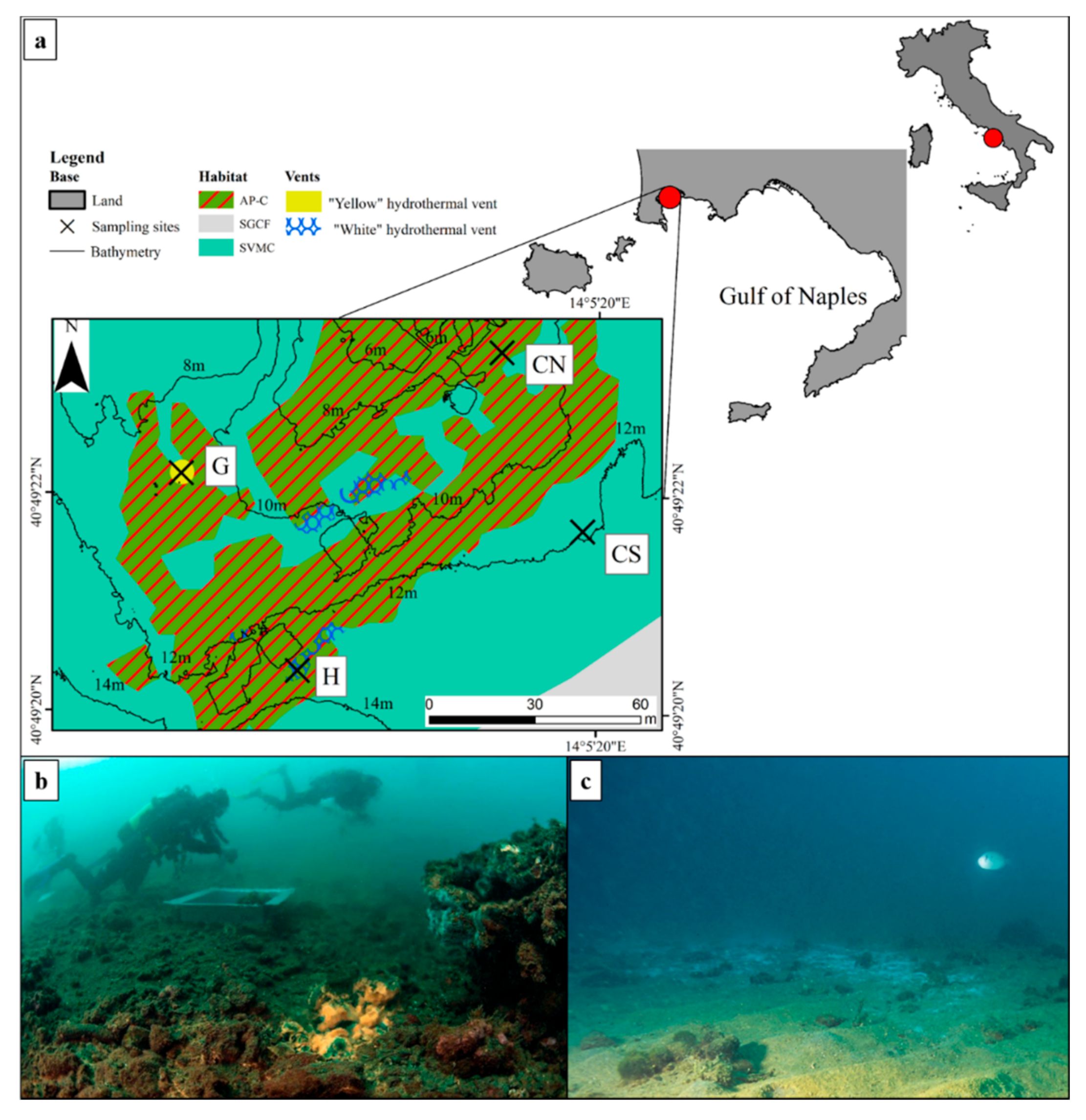
2.1. Study Area

The study area is located in the north-west side of the Gulf of Naples (Italy, south Tyrrhenian Sea) within the Underwater Archeological Park of Baia MPA. Since 2002 the MPA protects the coastline consisting of beaches and tuff cliffs shaped by volcanic activity, evident for both bradyseism phenomena and hydrothermal vents [33]. The interaction between natural processes and human activities produced a natural environment characterized by a strong interdigitation between photophilous and sciaphilous populations (AP-C). Superficial muddy sands in sheltered-water habitats (SVMC), enriched with fragments of carbonate exoskeletons of benthic organisms, are common in the sampling area. Coarse sands and fine gravels mixed by the waves habitat (SGCF) [34,35] is also present below 15 m depth.
The sampled area, named “Secca delle Fumose” (Figure 1a), is characterized by two vent typologies, and environmental parameters featuring each sampled site are shown in Table 1 [36,37]. The Geyser (G) site is a vent characterized by water emission reaching ~80 °C at the outlet, while at a distance of 20 cm from the center the sediments temperature is around 30 °C with a pH of 8. Rocky substrate surrounding the geyser are covered by yellow sulfurous deposits (Figure 1b), soft bottoms among the rocks are characterized by around 30% of TOC, and S2−, SO42−, Mg2+, Zn2+, and Pb2+ are the most abundant ions detected in their interstitial water.
The hydrothermal (H) vent site is characterized by carbon dioxide (CO2) bubbles and its sediments show an almost homogenous temperature of ~37 °C with a pH of 7.5. This site is characterized by a wide, white microbial mat (Figure 1c) on both rocky and sand bottoms, determining ~35% of TOC and Na+, NO3, and Pb2+ are the most abundant ions detected in their interstitial water.
At the control/inactive sites located at the north (CN) and at the south (CS) of the study area, approximately 100 m from respectively G and H, water and gases emissions are not present, sediments temperature is around 22 °C with a pH of 8.1. Sediments are characterized by around 17.5% of TOC and the most abundant ions in interstitial water are NO3, SO42−, Zn2+, and Pb2+.

2.2. Sampling Campaign and Data Analysis
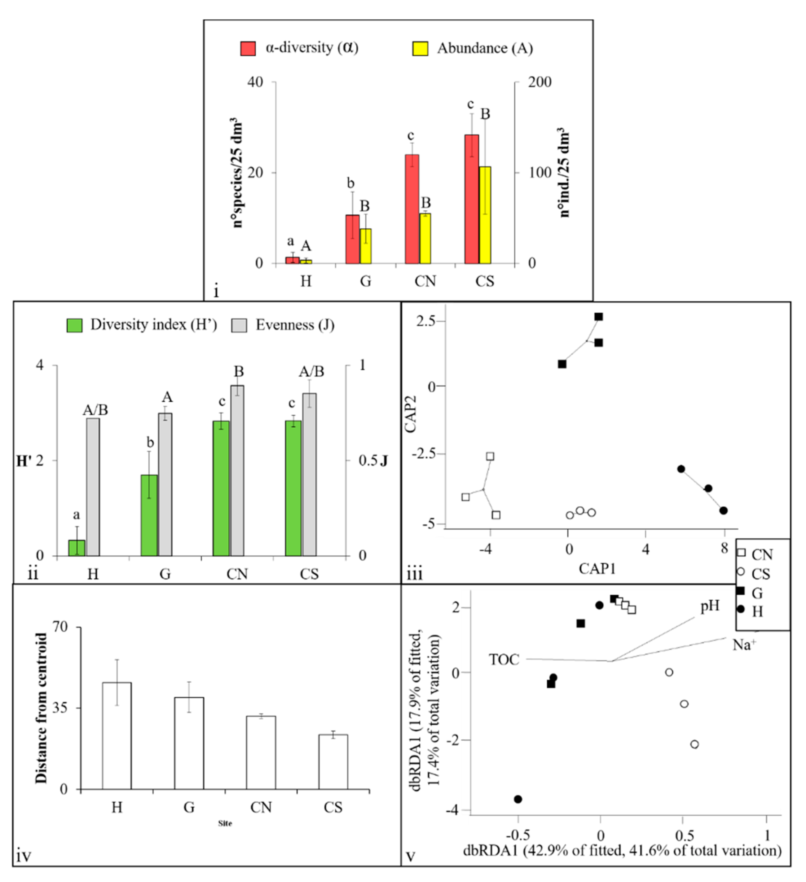
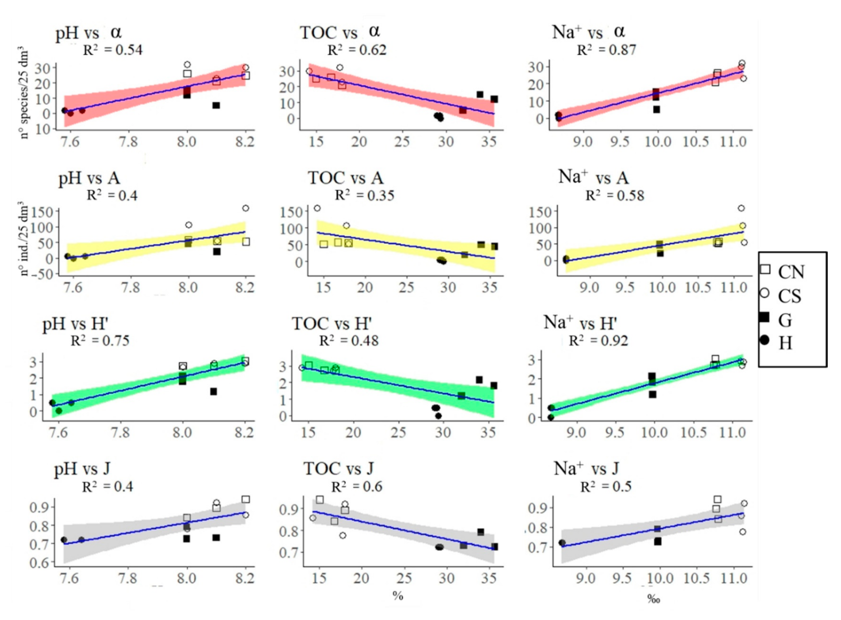
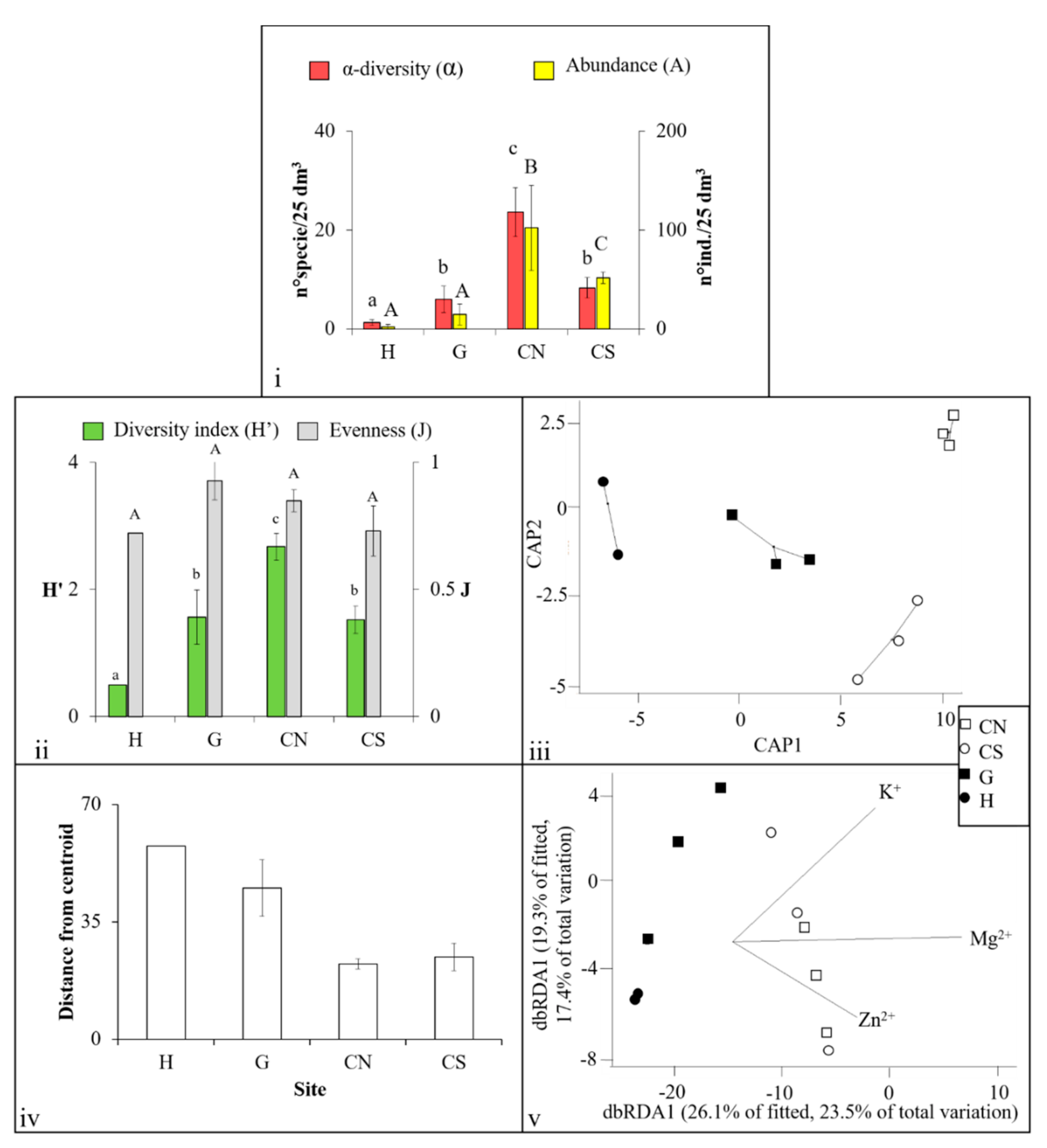
A macro- and meiofauna sampling campaign was performed in October 2016 in H, G, CN, and CS sites. All samples were collected in the same habitat: SVMC enriched with fragments of carbonate exoskeletons of benthic organisms.
Macrofauna samples were obtained at each site by scuba-diving through an air-lift pump equipped with a 0.5 mm nylon mesh size bag within a 50 cm × 50 cm frame, reaching a depth of 10 cm in the sediment (for further information on methodology see [36]).
Meiofauna samples were collected at each site by scuba-diving through cylindrical corers with a radius of 2.75 cm and reaching a depth of 10 cm in the sediment (for further information on methodology see [37]).
Mollusca (M), Polychaeta (P), Crustacea (C) (hereafter called macrofauna), and Nematoda (N) (hereafter called meiofauna) assemblages were the main taxa considered in the present study, being representative of more than the 80% of the total sampled organisms [36,37]. They were analyzed separately in order to describe each assemblage and to assess their β-diversity (measured as small-scale heterogeneity among sample replicates).
Descriptive analysis takes into account synecological indices: α-diversity, measured as species/taxa richness (αM, P, C = n° of species on 25 dm3; αN = n° of taxa on 0.25 dm3), abundances (AM, P, C = n° of individuals on 25 dm3; AN = n° of individuals on 0.25 dm3), diversity (H’, estimated by Shannon-Weaver index), and evenness (J, estimated by Pielou index).
Distance-based permutation univariate analysis of variances (PERMANOVA) [41] was based on synecological indices’ Euclidian distances [42] and each term in the analysis was tested by 4999 random permutations. Post hoc pair-wise comparisons using the PERMANOVA t-statistic and 4999 permutations were also conducted if necessary.
PERMANOVA multivariate analyses were carried out on abundances, in order to test for differences in assemblage structure due to environmental characteristics of each sampled site [experimental design involved one factor Site (Si, fixed, four levels) with n = 3]. Prior to the analyses data were log(x+1) transformed to reduce the weight of scanty taxa. All multivariate analyses were based on Bray–Curtis similarity, and each term in the analysis was tested by 4999 random permutations [43,44]. Post hoc pair-wise comparisons using the PERMANOVA t-statistic and 4999 permutations were also conducted if necessary. Multivariate patterns were visualized through Canonical Analyses of Principal coordinates (CAP) [45] of sites’ elements. Permutation tests of multivariate dispersion (PERMDISP) [46], a measure of β-diversity based on Bray–Curtis similarity matrices, were also performed for the term Si to investigate possible effects of environmental characteristics on small-scale heterogeneities among assemblages (heterogeneities are measured as mean ± SD distance of sites replicates from the centroid of the cluster they form). All analyses were performed using r-project software [47] with BiodiversityR package [48].
Environmental data measured at each site and reported in Table 1 [36], are here related to β-diversity measures of macro- and meiofauna assemblages. In particular, a distance-based linear modelling (DistLM) [49] using step-wise as selection procedure and adjusted R2 (hereafter called only R2) as selection criterion were performed in order to find correlations among the distances from the centroids in each site and environmental data. Relations between assemblage heterogeneities and environmental variables that significantly affect β-diversity were visualized through distance-based redundancy analysis (dbRDA) [50].
Finally, environmental parameters that significantly affect β-diversity were related to synecological indices through a linear regression model in order to assess their effects on assemblages structures. For each pair composed by environmental parameters (independent variable)/synecological index (dependent variable) the R2 was calculated to find possible correlations among synecological indices and environmental parameters.

3. Results

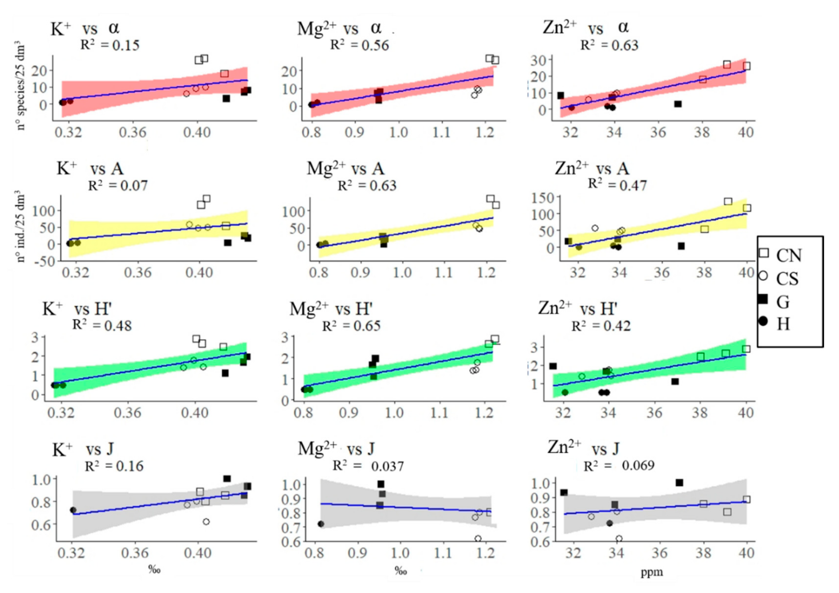
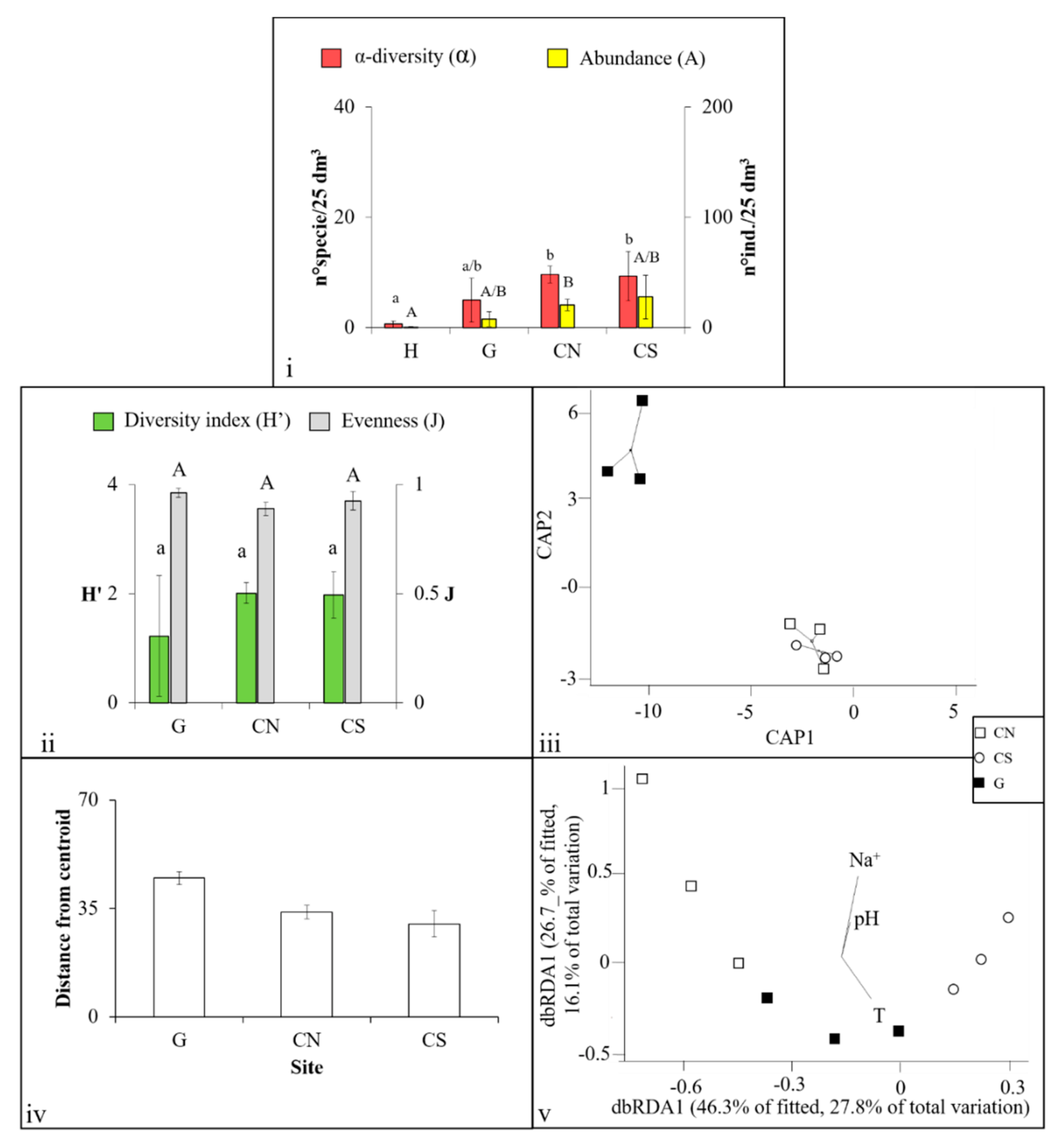
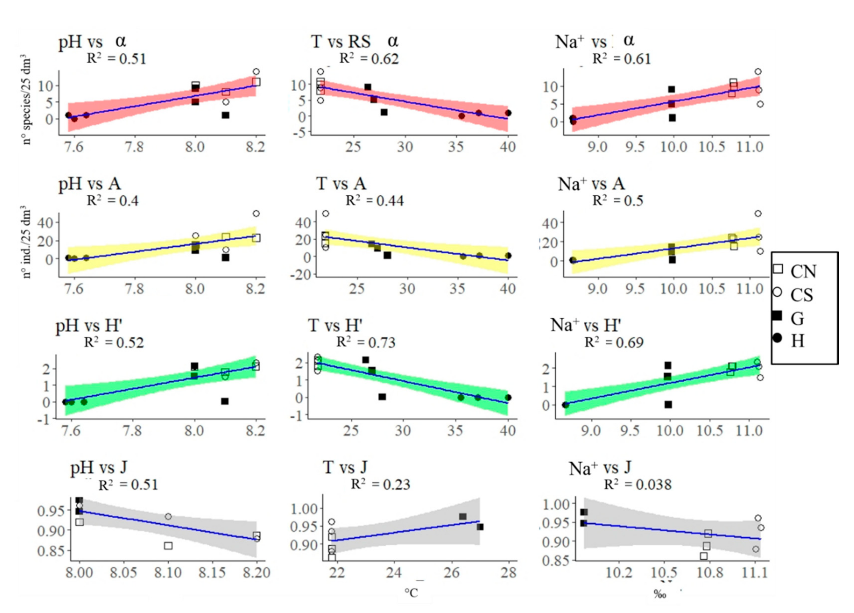
3.1. Mollusca Assemblages

The list of Mollusca collected in the four sites is shown in Supplementary Material (A).
The highest numbers of Mollusca species and individuals were detected at CS (αCS = 28.33 ± 4.76 species/25 dm3; ACS = 106.67 ± 52.50 individuals/25 dm3) while the lowest were found at H (αH = 1.33 ± 2.15 species/25 dm3; AH = 3.33 ± 2.89 individuals/25 dm3). α-diversity showed significant differences (p < 0.001) between hydrothermal vents sites and control/inactive sites, while abundances showed significant differences (p < 0.05) between H and the other sites (Figure 2i).
The highest values of diversity index and evenness were detected in CN and CS (H’CN = 2.83 ±0.17, JCN = 0.89 ± 0.05; H’CS = 2.83 ±0.12, JCS = 0.85 ± 0.07) while the lowest were found in in H and G (H’H = 0.33 ±0.28, JH = 0.72 ± 0.00; H’G = 1.70 ± 0.48, JG = 0.74 ± 0.03). The diversity index showed significant differences between the hydrothermal vents sites and control/inactive sites (p < 0.01) while evenness showed a significant difference between CN and G (p < 0.05) (Figure 2ii).
PERMANOVA analyses show significant differences between sites (p < 0.01); in particular the pair-wise test highlights significant differences between: H and control/inactive sites (pH,CN = 0.043; pH,CS = 0.031), and G and CN (p = 0.043). CAP analysis shows four different clusters separating the four levels composing the factor Site (Figure 2iii). PERMDISP does not show significant differences between small-scale heterogeneities of Mollusca assemblages but H is characterized by the greatest mean distance (d = 46.121 ± 9.893), while the lowest value belongs to the CS site (d = 23.551 ± 1.594) (Figure 2iv).
In addition to S2− (p = 0.036), detected only in G, DistLM shows that Mollusca heterogeneities at H and G are significantly and inversely affected by pH (p = 0.039; R2 = 0.74) and Na+ (p = 0.008; R2 = 0.65) and directly affected by TOC (p = 0.023; R2 = 0.71) that explain, altogether, about 60% of total variation (Figure 2v).
In Figure 3 correlations between environmental parameters and synecological indices that significantly affect Mollusca heterogeneities are shown. In particular, pH is always directly related to synecological indices showing the highest correlation with H’ (R2 = 0.75); TOC is always inversely related to synecological indices showing the highest correlation with α (R2 = 0.62) and J (R2 = 0.6); Na+ is always directly related to synecological indices showing the highest correlation with α (R2 = 0.87) and H’ (R2 = 0.92).

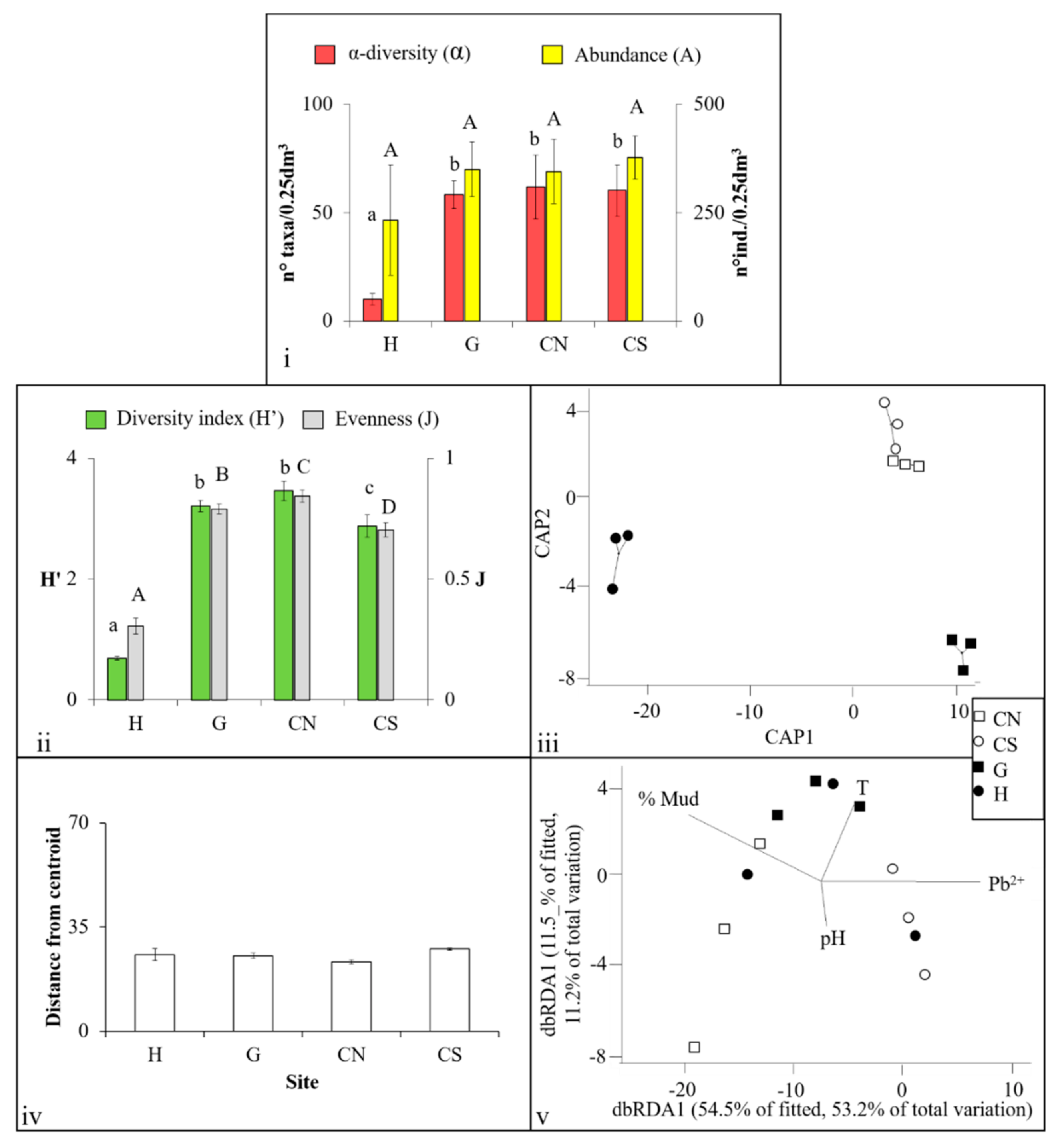
3.2. Polychaeta Assemblages

The list of Polychaeta collected in the four sites is shown in Supplementary Material (B).
The highest numbers of Polychaeta species and individuals were detected at CN (αCN = 23.67 ± 4.93 species/25 dm3; ACN = 102.33 ± 42.92 individuals/25 dm3) while the lowest were found at H (αH = 1.33 ± 0.57 species/25 dm3; AH = 2.33 ± 2.31 individuals/25 dm3). α-diversity showed significant differences (p < 0.01) between hydrothermal vents sites and control/inactive sites except between G and CS; while abundances showed significant differences (p < 0.001) between all sites except between those characterized by hydrothermal vents (Figure 4i).
The highest value of diversity index was detected in CN (H’CN = 2.67 ± 0.21) while the highest value of evenness was detected in G (JG = 0.92 ± 0.07). The lowest value of diversity index was detected in H (H’H = 0.5 ± 0.00) while the lowest values of evenness were found in both H and CS (JH = 0.72 ± 0.00, JCS = 0.73 ± 0.09). The diversity index did not show significant differences. Evenness showed significant differences between all sites (p < 0.05) except between G and CS (Figure 4ii).
PERMANOVA analyses show significant differences between sites (p < 0.01) although pair-wise test highlights significant differences only between the CN and CS sites (p = 0.012). CAP analysis shows four different clusters separating the four levels composing the factor Site (Figure 4iii). PERMDISP does not show significant differences among small-scale heterogeneities of Polychaeta assemblages but site H is characterized by the greatest mean distance (d = 57.735 ± 0.1), while the lowest value was recorded at site CN (d = 22.527 ± 1.568) (Figure 4iv).
DistLM shows that Polychaeta heterogeneities at H and G are significantly and inversely correlated to Mg2+ (p = 0.001; R2 = 0.92), Zn+ (p = 0.046; R2 = 0.56), and K+ (p = 0.014; R2 = 0.42), which explain, altogether, about 40% of the total variation (Figure 4v).
In Figure 5, correlations between environmental parameters and synecological indices that significantly affect Polychaeta heterogeneities are shown. In particular K+ is always directly related to synecological indices although with low value of R2 for which the highest is related to H’ (R2 = 0.48); Mg2+ is directly related to α, A, and H’ showing almost the same R2 (about 0.6) and inversely very weakly related to J (R2 = 0.037); Zn2+ is directly related to α, A, and H’, showing the highest correlation with α (R2 = 0.63), while a very low inverse relation is detected with J (R2 = 0.069).

3.3. Crustacea Assemblages

The list of Crustacea species collected in the four sites is shown in Supplementary Material (C).
The highest number of Crustacea species was recorded at CN (αCN = 9.66 ± 1.52 species/25 dm3) and the highest number of individuals was found at CS (ACN = 28 ± 19.67 individuals/25 dm3), while both the lowest number of species and individuals were detected at H (αH = 0.67 ± 0.58 species/25 dm3; AH = 0.67 ± 0.57 individuals/25 dm3). α-diversity showed significant differences (p < 0.05) between H and the control/inactive sites, while abundances exhibited significant differences (p < 0.05) only between the H and CN sites (Figure 6i).
Diversity and evenness indices were not calculated in the H site, since only one single species with one individual was recorded in two replicates. The highest value of diversity index was detected in CN (H’CN = 2.01 ± 0.19) and the lowest in G (H’G = 2.01 ± 0.19). The highest value of evenness was detected in G (JG = 0.96 ± 0.02) and the lowest in CN (JCN = 0.88 ± 0.03). Neither diversity and evenness indices sowed significant differences between sites (Figure 6ii).
PERMANOVA analyses were performed only among G and control/inactive sites since the low number of Crustacea species and individuals at site H did not allow the use of Bray–Curtis similarity.
The G and control/inactive sites show significant differences (p < 0.01; in particular pG,CN = 0.043; pG,CS = 0.033) as confirmed by CAP analysis that shows two clusters: one polarized on the positive area of CAP2 and composed by G replicates, and one polarized on the negative area of CAP2 and composed by control/inactive site replicates (Figure 6iii). PERMDISP does not show significant differences between small-scale heterogeneities of Crustacea assemblages, but the G site is characterized by the greatest mean distance (d = 44.828 ± 2.108), while the lowest value belongs to the CS site (Figure 6iv).
DistLM shows that Crustacea heterogeneities at G are significantly and inversely correlated to pH (p = 0.024; R2 = 0.73), Na+ (p = 0.002; R2 = 0.91) and directly affected by temperature (p = 0.012; R2 = 0.86), which explain, altogether, about 44% of the total variation (Figure 6v).
In Figure 7, correlations between environmental parameters and synecological indices that significantly affect Crustacea heterogeneities are shown. In particular, pH is directly related to α, A, and H’, showing almost the same R2 (about 0.5), and inversely related to J (R2 = 0.51); T is inversely related to α, A, and H’, showing the highest correlation with H’ (R2 = 0.73), and directly related to J (R2 = 0.23); Na+ is directly related to α, A, and H’, showing almost the same R2 (about 0.69), and inversely related to J (R2 = 0.038).

3.4. Nematoda Assemblages

The list of Nematoda taxa collected at the four sites is shown in Supplementary Material (D).
The highest number of Nematoda taxa was detected at CN (αCN = 62 ± 14.79 taxa/0.25 dm3) and the highest number of individuals was detected at CS (AG = 377 ±49.67 individuals/0.25 dm3) while the lowest numbers of species and individuals were detected at H (αH = 10 ±2.64 taxa/0.25 dm3; AH = 233.33 ±127.18 individuals/0.25 dm3). α-diversity showed significant differences (p < 0.05) between H and the other sites, while abundances did not show significant differences (Figure 8i).
The highest values of diversity and evenness indices were detected in CN and G (H’CN = 3.4 ± 0.15, JCN = 0.78 ± 0.02; H’G = 3.2 ± 0.09, JG = 0.84 ± 0.02) sites, while the lowest were found in H (H’H = 0.69 ± 0.03, JH = 0.30 ± 0.03). The diversity index showed significant differences between all sites (p < 0.05) except between G and CN. Evenness showed significant differences between all sites (p < 0.05) (Figure 8ii).
PERMANOVA analyses show significant differences between sites (p < 0.01)—in particular, the pair-wise test highlights significant differences between H and other sites (pH,CN = 0.0054, pH,CS = 0.007, pH,G = 0.003). CAP analysis shows three clusters: one polarized on the negative area of both CAP1 and CAP2, composed by H replicates; one polarized on the positive area of CAP1 and the negative area of CAP2, composed by G replicates; and one polarized on positive area of both CAP1 and CAP2, composed by control/inactive site replicates (Figure 8iii). PERMDISP does not show significant differences between small-scale heterogeneities of Nematoda assemblages whose distances are similar among the four sites (Figure 8iv).
DistLM shows that Nematoda heterogeneities at sites H and G are significantly and inversely correlated to pH (p = 0.028, R2 = 0.66) and to the % of mud (p = 0.008, R2 = 0.54), and directly correlated to Pb+ (p = 0.011, R2 = 0.737) and temperature (p = 0.032, R2 = 0.79), which explain, altogether, about 65% of the total variation (Figure 8v).
In Figure 9, correlations between environmental parameters and synecological indices that significantly affect Nematoda heterogeneities are shown. In particular pH is always directly related to synecological indices showing the highest correlations with α (R2 = 0.71), H’ (R2 = 0.80) and J (R2 = 0.79); T is always inversely related to synecological indices showing the highest correlations with α (R2 = 0.76), H’ (R2 = 0.80), and J (R2 = 0.75); Pb2+ is inversely related to to synecological indices showing the highest correlations with J (R2 = 0.49). Mud always shows a very weakly correlation with synecological indices.

4. Discussions

4.1. Effects of Acidification on β-Diversity

The present study aims at detecting the possible effects of hydrothermal vents, located within an MPA, on β-diversity of soft-bottom meiobenthic and macrobenthic assemblages. Faunistic results from the sediment samples collected at each site were divided in four main sub-assemblages that represent the vast majority of macrobenthic communities (Mollusca, Polychaeta, and Crustacea populations) and meiobenthic communities (Nematoda populations). Coherently with previous studies [36,37] the lowest α-diversity and abundance were detected at site H, followed by the G site. The control/inactive sites were characterized by soft-bottom community values comparable with other investigations in similar habitats (i.e., [51,52,53,54,55]). In our study, PERMANOVA highlighted significant differences between the hydrothermal vents and the CN and CS sites, while PERMDISP did not show significant differences between small-scale heterogeneities (differences between same-site replicates) [14]. In classical BACI (Before and After Controls Impacts) studies [56] high small-scale heterogeneities are related to lowly disturbed areas since an impact often tends to homogenize community structures, lowering redundancy [57,58] and resilience capacity [18,59]. However, this is not always true since it may depend on what kind of species or taxa compose the assemblages. Indeed, a recent paper [60] shows evidence that good quality of coralligenous assemblages results in more homogeneous assemblages since the dominance of sessile species homogenizes community structures over a long timescale, not allowing the easy settlement of minor taxa. In the present investigation, site H showed the highest heterogeneity values although composed by the lowest number of taxa at both macro and meiobenthic level. This can be explained considering that the low number of taxa and individuals at H are represented by tolerant species, such as Tritia cuvierii (Payraudeau, 1826) and the sibling Capitella capitata (Fabricius, 1780), that can survive in such extreme conditions as those created by the presence of CO2 [36,61]. Most macrobenthic and meiofaunal species recorded at site H are also present at site G but not at the control/inactive sites, confirming that hydrothermal vent conditions are the drivers shaping the structure of these benthic assemblages. Although meiobenthic communities are generally more structured than macrobenthic ones, site H was characterized by some dominant Nematoda genera such as Daptonema (Cobb, 1920) and Oncholaimus (Dujardin, 1845) [37] that, as previously shown, exhibit high tolerance to CO2 [62,63].
In the present investigation some abiotic parameters, such as: pH, temperature, cation concentrations, etc., affected β-diversity, (assessed through small-scale heterogeneity measures among replicates). In particular, distLM show that temperature is significantly related to crustacean and nematodean assemblages, while acidification (measured as variation of either pH or ions concentrations) affects both macro- and meio-assemblages. Such findings are coherent with previous studies that show how the increase in temperature and the decrease in pH synergistically act on assemblages’ structures [28,64]. Indeed, on one hand, low α-diversity and abundances of macrobenthic assemblages are related to the temperature rising, that eliminates low-resilient species, primarily crustacean, determining: reduction in growth and survival rates [65], and thus destructuring the community and the evenness among species. On the other hand, high heterogeneity is strictly related to the acidified environments [66,67], highlighted by low values of pH and by the presence of some cations resulting from seawater and sediments (Na+, Mg+ and K+) [68]. It is known, as previously shown by Linares et al. (2015) [32] that even a small decrease of pH may lead to dramatic shifts in highly diverse and structurally complex benthic systems. Acidification affects sensitive macrobenthic species that completely disappear, decreasing redundancy and generating available niches for other more tolerant species. This is particularly evident with Mollusca α-diversity and abundances, which are correlated with TOC at the G and H sites, as shown by the disappearance, at these sites, of Hiatella arctica (Linnaeus, 1767) (abundant in control/inactive sites) that, as also shown in other studies (i.e., [69]) cannot survive since acidification affects their shell texture [70], calcification [31] and growth rate [30].

4.2. Assemblages’ Strategies to Mitigate Acidification Effects

While previous studies showed that seawater acidification causes important changes at species/taxa (α-diversity) level (i.e., [25,71]), to our knowledge this study may be the first one highlighting that β-diversity might be directly related to acidification. The protection level of this MPA excludes marked anthropic impacts, thus confirming that acidification, although increasing the heterogeneity in H and G sites, may lower β-diversity coherently with the pH gradient that, in turn, generates a loss of redundancy. The highest heterogeneity present at H and, to a lesser extent, at G is due to microhabitats available among sediment particles. Acidification might inhibit interstitial species’ existence; however, they may be able to find micro-areas where they can live if the small-scale environmental conditions are not so extreme [72]. The concept of microhabitat may change when we consider macro- or meiobenthic assemblages. Macrobenthic species, due to their larger size, tend to be borrowers (endobenthic) rather than interstitial (mesobenthic), like most meiofauna; consequently, they do not occupy interstitial spaces. This causes high dispersions of macrofauna and thus great heterogeneity also for poorly structured assemblages. Conversely, meiofauna, and Nematoda in particular, find more available microhabitats in the interstitial space, due to their smaller size, giving rise to well-structured and diversified assemblages [73,74,75] and, thus, increasing synecological values and maintaining unchanged β-diversity.
The present investigation shows that more heterogeneous assemblages may be related to hydrothermal vents where the acidification effects are more evident, though reducing number of species and destructuring the communities. Thus, in these conditions high heterogeneity is representative of low β-diversity and, consequently, low resilience capacity due to the loss of redundancy at the H and G sites, since benthic organisms are forced to use only the microhabitat where extreme conditions are not present. In particular, this is more evident for macrobenthic than meiobenthic assemblages since for the former the likelihood to find survival habitats among grains of sand and mud is very scanty.

5. Conclusions

According to the results we obtained in this study, we can maintain that acidification affects not only benthic community structures but also their β-diversity and, in turn, their resilience capacity. These effects, here related to a particular shallow, acidified, volcanic environment at SdF may be extended to other acidified environments due, for instance, to climate changes. Therefore, it may be useful to measure community resilience capacity of soft-bottom assemblages in order to value, at the same time, the severity of climate change effects. In this study, high heterogeneities among replicates, linked to low synecological indices, may be indicators of low resilience capacity due to environmental changes that occurred so quickly that communities could not recover to a more stable climax stage. Finally, as previously shown in other studies, high heterogeneity is not always an indicator of high β-diversity and its values should be considered in the context of the study area. Thus, in extreme marine environments, where several factors exert limiting effects on many species, the heterogeneity, considered as new opportunities for some species but also as negative conditions for other ones, may be associated with lower biodiversity values.

Supplementary Materials

The supplementary materials are available online at https://0-www-mdpi-com.brum.beds.ac.uk/1424-2818/12/12/464/s1.

Author Contributions

Writing Original Draft: L.A.; Conceptualization: L.A., D.Z. and R.S.; Taxonomic analyses: E.B. and L.D.; Chemical analyses: E.C.; Statistical analyses: L.A.; Supervision: D.Z.; R.S. and G.F.R.; Funding Acquisition, D.Z. All authors reviewed the manuscript. All authors have read and agreed to the published version of the manuscript.

Funding

Financial support was provided by the project “Prokaryote-nematode Interaction in marine extreme envirONments: a uniquE source for ExploRation of innovative biomedical applications” (PIONEER) funded by the Total Foundation and IFREMER (2016–2019) and by the project Boost Europe—ERC “Extreme marine nematoDes: moDel orgAnisms for a Journey toward the origin and Evolution of metazoan life in our changing planet” (EDDAJE) funded by the Brittany Region and IFREMER (2019).

Acknowledgments

We are grateful to Soprintendenza of the Underwater Archeological Park of Baia (prot. 5667, 24/10/2016) for the authorization to sampling. We are thankful to Guido Villani for assistance during the underwater sampling and permission to use photos that enriched the manuscript. Thanks are also due to the diving center Centro SUB Pozzuoli (Guglielmo Fragale) for support field activities and Aurélie Tasiemski and Céline Boidin-Wichlacz for helping in sampling activities. We also thank the reviewers for the suggestions and comments. We are indebted to Jeroen Ingels (Florida State University) for useful discussions.

Conflicts of Interest

The authors declare that they have no competing interests. The founding sponsors had no role in the design of the study; in the collection, analyses, or interpretation of data; in the writing of the manuscript, or in the decision to publish the results.

References

  1. Donnarumma, L.; Sandulli, R.; Appolloni, L.; Sánchez-Lizaso, J.L.; Russo, G.F. Assessment of structural and functional diversity of mollusc assemblages within vermetid bioconstructions. Diversity 2018, 10, 96. [Google Scholar] [CrossRef] [Green Version]
  2. Donnarumma, L.; Sandulli, R.; Appolloni, L.; Russo, G.F. Assessing molluscs functional diversity within different coastal habitats of Mediterranean marine protected areas. Ecol. Quest. 2018, 29, 35–51. [Google Scholar]
  3. Gerlach, S.A. On the importance of marine meiofauna for benthos communities. Oecologia 1971, 6, 176–190. [Google Scholar] [CrossRef]
  4. Castelli, A.; Lardicci, C.; Tagliapietra, D. Soft-bottom macrobenthos. In Mediterranean Marine Benthos: A Manual of Methods for Its Sampling and Study; Gambi, M.C., Dappiano, M., Eds.; S.I.B.M—Società Italiana di Biologia Marina: Genova, Italy, 2003; pp. 99–132. [Google Scholar]
  5. Shmida, A.V.I.; Wilson, M. V Biological determinants of species diversity. J. Biogeogr. 1985, 12, 1–20. [Google Scholar] [CrossRef]
  6. Hoegh-Guldberg, O.; Bruno, J.F. The impact of climate change on the world’s marine ecosystems. Science 2010, 328, 1523–1528. [Google Scholar] [CrossRef] [PubMed]
  7. Bruno, J.F.; Bertness, M. Habitat modification and facilitation in benthic marine communities. In Marine Community Ecology; Bertness, M., Gaines, S., Hay, M., Eds.; Sinauer Associates: Sunderland, MA, USA, 2001; pp. 201–218. [Google Scholar]
  8. Buonocore, E.; Donnarumma, L.; Appolloni, L.; Miccio, A.; Russo, G.F.; Franzese, P.P. Marine natural capital and ecosystem services: An environmental accounting model. Ecol. Modell. 2020, 424, 109029. [Google Scholar] [CrossRef]
  9. Buonocore, E.; Appolloni, L.; Russo, G.F.; Franzese, P.P. Assessing natural capital value in marine ecosystems through an environmental accounting model: A case study in Southern Italy. Ecol. Modell. 2020, 419, 108958. [Google Scholar] [CrossRef]
  10. Rendina, F.; Bouchet, P.J.; Appolloni, L.; Russo, G.F.; Sandulli, R.; Kolzenburg, R.; Putra, A.; Ragazzola, F. Physiological response of the coralline alga Corallina officinalis L. to both predicted long-term increases in temperature and short-term heatwave events. Mar. Environ. Res. 2019, 150, 104764. [Google Scholar] [CrossRef]
  11. O’Leary, J.K.; Micheli, F.; Airoldi, L.; Boch, C.; De Leo, G.; Elahi, R.; Ferretti, F.; Graham, N.A.J.; Litvin, S.Y.; Low, N.H.; et al. The resilience of marine ecosystems to climatic disturbances. Bioscience 2017, 67, 208–220. [Google Scholar] [CrossRef]
  12. Sanda, T.; Hamasaki, K.; Dan, S.; Kitada, S. Expansion of the Northern Geographical Distribution of Land Hermit Crab Populations: Colonization and Overwintering Success of Coenobita purpureus on the Coast of the Boso. Zool. Stud. 2019, 58, e25. [Google Scholar]
  13. Kao, K.; Keshavmurthy, S.; Tsao, C.; Wang, J.; Chen, A. Repeated and Prolonged Temperature Anomalies Negate Symbiodiniaceae Genera Shuffling in the Coral Platygyra verweyi (Scleractinia; Merulinidae). Zool. Stud. 2018, 57, 1–14. [Google Scholar]
  14. Anderson, M.J.; Crist, T.O.; Chase, J.M.; Vellend, M.; Inouye, B.D.; Freestone, A.L.; Sanders, N.J.; Cornell, H.V.; Comita, L.S.; Davies, K.F.; et al. Navigating the multiple meanings of β diversity: A roadmap for the practicing ecologist. Ecol. Lett. 2011, 14, 19–28. [Google Scholar] [CrossRef] [PubMed]
  15. Baeten, L.; Vangansbeke, P.; Hermy, M.; Peterken, G.; Vanhuyse, K.; Verheyen, K. Distinguishing between turnover and nestedness in the quantification of biotic homogenization. Biodivers. Conserv. 2012, 21, 1399–1409. [Google Scholar] [CrossRef] [Green Version]
  16. Bevilacqua, S.; Plicanti, A.; Sandulli, R.; Terlizzi, A. Measuring more of Beta-diversity: Quantifying patterns of variation in assemblage heterogeneity. An insight from marine benthic assemblages. Ecol. Indic. 2012, 18, 140–148. [Google Scholar] [CrossRef]
  17. Appolloni, L.; Bevilacqua, S.; Sbrescia, L.; Sandulli, R.; Terlizzi, A.; Russo, G.F. Does full protection count for the maintenance of β-diversity patterns in marine communities? Evidence from Mediterranean fish assemblages. Aquat. Conserv. Mar. Freshw. Ecosyst. 2017, 27, 828–838. [Google Scholar] [CrossRef] [Green Version]
  18. Thrush, S.F.; Hewitt, J.E.; Cummings, V.J.; Norkko, A.; Chiantore, M. β-diversity and species accumulation in Antarctic coastal benthos: Influence of habitat, distance and productivity on ecological connectivity. PLoS ONE 2010, 5, e11899. [Google Scholar] [CrossRef]
  19. Thrush, S.F.; Hewitt, J.E.; Lohrer, A.M. Interaction networks in coastal soft-sediments highlight the potential for change in ecological resilience. Ecol. Appl. 2012, 22, 1213–1223. [Google Scholar] [CrossRef]
  20. Fritz, K.M.; Dodds, W.K. Resistance and resilience of macroinvertebrate assemblages to drying and flood in a tallgrass prairie stream system. Hydrobiologia 2004, 527, 99–112. [Google Scholar] [CrossRef]
  21. Townsend, C.R.; Hildrew, A.G. Species traits in relation to a habitat templet for river systems. Freshw. Biol. 1994, 31, 265–275. [Google Scholar] [CrossRef]
  22. Peterson, G.; Allen, C.R.; Holling, C.S. Ecological resilience, biodiversity, and scale. Ecosystems 1998, 1, 6–18. [Google Scholar] [CrossRef]
  23. Holling, C.S.; Schindler, D.W.; Walker, B.W.; Roughgarden, J. Biodiversity in the functioning of ecosystems: An ecological synthesis. In Biodiversity Loss: Economic and Ecological Issues; Perrings, C., Karl-Goran, M., Folke, C., Holling, C.S., Bengt-Owe, J., Eds.; Cambridge University Press: Cambridge, UK, 1995; pp. 44–83. [Google Scholar]
  24. Montefalcone, M.; Parravicini, V.; Bianchi, C.N. Quantification of coastal ecosystem resilience. Treatise Estuar. Coast. Sci. 2011, 10, 49–70. [Google Scholar]
  25. Hall-Spencer, J.M.; Rodolfo-Metalpa, R.; Martin, S.; Ransome, E.; Fine, M.; Turner, S.M.; Rowley, S.J.; Tedesco, D.; Buia, M.C. Volcanic carbon dioxide vents show ecosystem effects of ocean acidification. Nature 2008, 454, 96–99. [Google Scholar] [CrossRef] [PubMed] [Green Version]
  26. Gattuso, J.-P.; Hansson, L. Ocean Acidification; Oxford University Press: Oxford, UK, 2011; ISBN 0199591091. [Google Scholar]
  27. Wang, T.; Chan, T.; Chan, B.K.K. Diversity and community structure of decapod crustaceans at hydrothermal vents and nearby deep-water fishING grounds off Kueishan Island, Taiwan: A high biodiversity deep-sea area in the NW Pacific. Bull. Mar. Sci. 2013, 89, 505–528. [Google Scholar] [CrossRef]
  28. Chan, B.K.K.; Wang, T.; Chen, P.; Lin, C. Community Structure of Macrobiota and Environmental Parameters in Shallow Water Hydrothermal Vents off Kueishan Island, Taiwan. PLoS ONE 2016, 11, e0148675. [Google Scholar] [CrossRef] [PubMed] [Green Version]
  29. Donnarumma, L.; Lombardi, C.; Cocito, S.; Gambi, M.C. Settlement pattern of Posidonia oceanica epibionts along a gradient of ocean acidification: An approach with mimics. Mediterr. Mar. Sci. 2014, 15, 498–509. [Google Scholar] [CrossRef] [Green Version]
  30. Berge, J.A.; Bjerkeng, B.; Pettersen, O.; Schaanning, M.T.; Øxnevad, S. Effects of increased sea water concentrations of CO2 on growth of the bivalve Mytilus edulis L. Chemosphere 2006, 62, 681–687. [Google Scholar] [CrossRef]
  31. Gazeau, F.; Quiblier, C.; Jansen, J.M.; Gattuso, J.P.; Middelburg, J.J.; Heip, C.H.R. Impact of elevated CO2 on shellfish calcification. Geophys. Res. Lett. 2007, 34, 1–5. [Google Scholar] [CrossRef] [Green Version]
  32. Linares, C.; Vidal, M.; Canals, M.; Kersting, D.K.; Amblas, D.; Aspillaga, E.; Cebrián, E.; Delgado-Huertas, A.; Díaz, D.; Garrabou, J.; et al. Persistent natural acidification drives major distribution shifts in marine benthic ecosystems. Proc. R. Soc. B Biol. Sci. 2015, 282, 20150587. [Google Scholar] [CrossRef]
  33. Tedesco, D. I fluidi fumarolici sottomarini dell’era vulcanica napoletana: Cambiamenti globali, dinamiche vulcaniche e genesi dei fluidi, mitigazione del rischio vulcanico. In Proceedings of the Il Fuoco Dal Mare—Vulcanismo e Ambienti Sottomarini; Coiro, P., Russo, G.F., Eds.; Giannini Editore: Napoli, Italy, 2008; pp. 99–112. [Google Scholar]
  34. Appolloni, L.; Sandulli, R.; Vetrano, G.; Russo, G.F. Assessing the effects of habitat patches ensuring propagule supply and different costs inclusion in marine spatial planning through multivariate analyses. J. Environ. Manag. 2018, 214, 45–55. [Google Scholar] [CrossRef] [Green Version]
  35. Appolloni, L.; Sandulli, R.; Bianchi, C.N.; Russo, G.F. Spatial analyses of an integrated landscape-seascape territorial system: The case of the overcrowded Gulf of Naples, Southern Italy. J. Environ. Account. Manag. 2018, 6, 365–380. [Google Scholar] [CrossRef]
  36. Donnarumma, L.; Appolloni, L.; Chianese, E.; Bruno, R.; Baldrighi, E.; Guglielmo, R.; Russo, G.F.; Zeppilli, D.; Sandulli, R. Environmental and Benthic Community Patterns of the Shallow Hydrothermal Area of Secca Delle Fumose (Baia, Naples, Italy). Front. Mar. Sci. 2019, 6, 1–15. [Google Scholar] [CrossRef] [Green Version]
  37. Baldrighi, E.; Zeppilli, D.; Appolloni, L.; Donnarumma, L.; Chianese, E.; Russo, G.F.; Sandulli, R. Meiofaunal communities and nematode diversity characterizing the Secca delle Fumose shallow vent area (Gulf of Naples, Italy). PeerJ 2020, 8, 1–28. [Google Scholar] [CrossRef] [PubMed]
  38. Kenny, A.J.; Sotheran, I. Characterising the Physical Properties of Seabed Habitats. In Methods for the Study of Marine Benthos; Eleftheriou, A., Ed.; John Wiley & Sons: Chichester, West Sussex, UK, 2013; ISBN 1118542371. [Google Scholar]
  39. Schumacher, B.A. Methods for the Determination of Total Organic Carbon (TOC) in Soils and Sediments, NCEA-C-1282, 1st ed.; Schumacher, B.A., Ed.; US Environmental Protection Agency, Office of Research and Development: Washington, DC, USA, 2002.
  40. Chianese, E.; Tirimberio, G.; Riccio, A. PM2.5 and PM10 in the urban area of Naples: Chemical composition, chemical properties and influence of air masses origin. J. Atmos. Chem. 2019, 76, 151–169. [Google Scholar] [CrossRef]
  41. Anderson, M.J. A new method for non parametric multivariate analysis of variance. Austral Ecol. 2001, 26, 32–46. [Google Scholar]
  42. Terlizzi, A.; Anderson, M.J.; Fraschetti, S.; Benedetti-Cecchi, L. Scales of spatial variation in Mediterranean subtidal sessile assemblages at different depths. Mar. Ecol. Prog. Ser. 2007, 332, 25–39. [Google Scholar] [CrossRef] [Green Version]
  43. Anderson, M.J. Permutation tests for univariate or multivariate analysis of variance and regression. Can. J. Fish. Aquat. Sci. 2001, 58, 626–639. [Google Scholar] [CrossRef]
  44. Anderson, M.; Braak, C. Ter Permutation tests for multi-factorial analysis of variance. J. Stat. Comput. Simul. 2003, 73, 85–113. [Google Scholar] [CrossRef]
  45. Anderson, M.J.; Willis, T.J. Canonical Analysis of Principal Coordinates: A Useful Method of Constrained Ordination for Ecology. Ecology 2003, 84, 511–525. [Google Scholar] [CrossRef]
  46. Anderson, M.J.; Ellingsen, K.E.; McArdle, B.H. Multivariate dispersion as a measure of beta diversity. Ecol. Lett. 2006, 9, 683–693. [Google Scholar] [CrossRef]
  47. R Development Core Team, R. R: A Language and Environment for Statistical Computing. R Found. Stat. Comput. 2011, 1, 409. [Google Scholar]
  48. Kindt, R.; Coe, R. Tree Diversity Analysis: A Manual and Software for Common Statistical Methods for Ecological and Biodiversity Studie; World Agroforestry Centre (ICRAF): Nairobi, Kenya, 2005; ISBN 92 9059 179 X. [Google Scholar]
  49. Anderson, M.J. DISTLM v. 5: A FORTRAN computer program to calculate a distance-based multivariate analysis for a linear model. Dep. Stat. Univ. Auckl. N. Z. 2004, 10, 2016. [Google Scholar]
  50. Legendre, P.; Anderson, M.J. Distance-based redundancy analysis: Testing multispecies responses in multicfacorial ecological experiments. Ecol. Monogr. 1999, 69, 1–24. [Google Scholar] [CrossRef]
  51. Mastrototaro, F.; D’Onghia, G.; Tursi, A. Spatial and seasonal distribution of ascidians in a semi-enclosed basin of the Mediterranean Sea. J. Mar. Biol. Assoc. UK 2008, 88, 1053–1061. [Google Scholar] [CrossRef]
  52. Gambi, M.C.; Giangrande, A. Distribution of soft-bottom polychaetes in two coastal areas of the Tyrrhenian Sea (Italy): Structural analysis. Estuar. Coast. Shelf Sci. 1986, 23, 847–862. [Google Scholar] [CrossRef]
  53. Fanelli, E.; Lattanzi, L.; Nicoletti, L.; Tomassetti, P. Decapod crustaceans of Tyrrhenian Sea soft bottoms (central Mediterranean). Crustac. J. Crustac. Res. 2005, 78, 641. [Google Scholar]
  54. Gambi, M.C.; Conti, G.; Bremec, C.S. Polycliaete distribution, diversity and seasonality related to seagrass cover in shallow soft bottoms of the Tyrrhenian Sea (Italy). Sci. Mar. 1998, 62, 1–17. [Google Scholar]
  55. Cantone, G.; Fassari, G. Polychaetous annelids of soft-bottoms around the Gulf of Catania (Sicily). Comm. Int. Explor. Mer Mediterr. 1983, 28, 251–252. [Google Scholar]
  56. Smith, E.P. BACI Design. Wiley StatsRef Stat. Ref. Online 2014, 1, 141–148. [Google Scholar]
  57. Magurran, A.E.; Dornelas, M.; Moyes, F.; Gotelli, N.J.; McGill, B. Rapid biotic homogenization of marine fish assemblages. Nat. Commun. 2015, 6, 8405. [Google Scholar] [CrossRef] [Green Version]
  58. Séguin, A.; Gravel, D.; Archambault, P. Effect of disturbance regime on alpha and beta diversity of rock pools. Diversity 2014, 6, 1–17. [Google Scholar] [CrossRef]
  59. Thrush, S.F.; Hewitt, J.E.; Dayton, P.K.; Coco, G.; Lohrer, A.M.; Norkko, A.; Norkko, J.; Chiantore, M. Forecasting the limits of resilience: Integrating empirical research with theory. Proc. R. Soc. B Biol. Sci. 2009, 276, 3209–3217. [Google Scholar] [CrossRef] [PubMed] [Green Version]
  60. Appolloni, L.; Ferrigno, F.; Russo, G.F.; Sandulli, R. β-Diversity of morphological groups as indicator of coralligenous community quality status. Ecol. Indic. 2020, 109, 105840. [Google Scholar] [CrossRef]
  61. Martin, J.; Bastida, R. Life history and production of Capitella Capitata (Capitellidae: Polychaeta) in Río de La Plata Estuary (Argentina). Thalassas 2006, 22, 25–38. [Google Scholar]
  62. Nandan, S.B. Retting of coconut husk-a unique case of water pollution on the South West coast of India. Int. J. Environ. Stud. 1997, 52, 335–355. [Google Scholar] [CrossRef]
  63. Thiermann, F.; Vismann, B.; Giere, O. Sulphide tolerance of the marine nematode Oncholaimus campylocercoides—A result of internal sulphur formation? Mar. Ecol. Prog. Ser. 2000, 193, 251–259. [Google Scholar] [CrossRef]
  64. Hale, R.; Calosi, P.; Mcneill, L.; Mieszkowska, N.; Widdicombe, S. Predicted levels of future ocean acidifi cation and temperature rise could alter community structure and biodiversity in marine benthic communities. Oikos 2011, 120, 661–674. [Google Scholar] [CrossRef]
  65. Whiteley, N.M. Physiological and ecological responses of crustaceans to ocean acidification. Mar. Ecol. Prog. Ser. 2011, 430, 257–271. [Google Scholar] [CrossRef] [Green Version]
  66. Kerrison, P.; Hall-Spencer, J.M.; Suggett, D.J.; Hepburn, L.J.; Steinke, M. Assessment of pH variability at a coastal CO2 vent for ocean acidification studies. Estuar. Coast. Shelf Sci. 2011, 94, 129–137. [Google Scholar] [CrossRef] [Green Version]
  67. Vizzini, S.; Di Leonardo, R.; Costa, V.; Tramati, C.D.; Luzzu, F.; Mazzola, A. Trace element bias in the use of CO2 vents as analogues for low pH environments: Implications for contamination levels in acidified oceans. Estuar. Coast. Shelf Sci. 2013, 134, 19–30. [Google Scholar] [CrossRef]
  68. Widdicombe, S.; Dashfield, S.L.; McNeill, C.L.; Needham, H.R.; Beesley, A.; McEvoy, A.; Øxnevad, S.; Clarke, K.R.; Berge, J.A. Effects of CO2 induced seawater acidification on infaunal diversity and sediment nutrient fluxes. Mar. Ecol. Prog. Ser. 2009, 379, 59–75. [Google Scholar] [CrossRef] [Green Version]
  69. Chen, C.; Chan, T.Y.; Chan, B.K.K. Molluscan diversity in shallow water hydrothermal vents off Kueishan Island, Taiwan. Mar. Biodivers. 2018, 48, 709–714. [Google Scholar] [CrossRef]
  70. Seibel, B.A.; Walsh, P.J. Biological impacts of deep-sea carbon dioxide injection inferred from indices of physiological performance. J. Exp. Biol. 2003, 206, 641–650. [Google Scholar] [CrossRef] [Green Version]
  71. Fabricius, K.E.; Langdon, C.; Uthicke, S.; Humphrey, C.; Noonan, S.; De’ath, G.; Okazaki, R.; Muehllehner, N.; Glas, M.S.; Lough, J.M. Losers and winners in coral reefs acclimatized to elevated carbon dioxide concentrations. Nat. Clim. Chang. 2011, 1, 165. [Google Scholar] [CrossRef]
  72. Somerfield, P.J.; Dashfield, S.L.; Warwick, R.M. Three-dimensional spatial structure: Nematodes in a sandy tidal flat. Mar. Ecol. Prog. Ser. 2007, 336, 177–186. [Google Scholar] [CrossRef] [Green Version]
  73. Dashfield, S.L.; Somerfield, P.J.; Widdicombe, S.; Austen, M.C.; Nimmo, M. Impacts of ocean acidification and burrowing urchins on within-sediment pH profiles and subtidal nematode communities. J. Exp. Mar. Bio. Ecol. 2008, 365, 46–52. [Google Scholar] [CrossRef]
  74. Bevilacqua, S.; Sandulli, R.; Plicanti, A.; Terlizzi, A. Taxonomic distinctness in Mediterranean marine nematodes and its relevance for environmental impact assessment. Mar. Pollut. Bull. 2012, 64, 1409–1416. [Google Scholar] [CrossRef]
  75. Semprucci, F.; Balsamo, M.; Appolloni, L.; Sandulli, R. Assessment of ecological quality status along the Apulian coasts (eastern Mediterranean Sea) based on meiobenthic and nematode assemblages. Mar. Biodivers. 2018, 48, 105–115. [Google Scholar] [CrossRef]
Figure 1. (a) Geomorphological/Habitat map of “Secca delle Fumose”. AP-C: intedigitaton between photophilous and sciaphilous habitats; SVMC: superficial muddy sands in sheltered-water habitats enriched with fragments carbonate exoskeletons of benthic organisms; SGCF: coarse sands and fine gravels mixed by the waves habitat. Sampling sites are also shown: (b) G site is characterized by a geyser of sulfurous hot water emissions that determine a yellow mat; (c) H site is characterized by carbon dioxide emissions with formation of a white bacterial mat; CN, and CS are the control/inactive sites.
Diversity 12 00464 g001
Figure 2. (i) α-diversity (α) and abundances (A) trends of Mollusca assemblages, (ii) diversity (H’) and evenness (J) indices trends of Mollusca assemblages. Bars with different letters (a, b, c or A, B) are related to sites showing significant differences (p < 0.05). (iii) Canonical Analysis of Principal coordinates (CAP) for the factor Site: straight lines are related to distances of each site replicates from their cluster centroid, formally explained in (iv): mean (±SE) multivariate dispersion (PERMDISP, small-scale heterogeneities) of the Mollusca assemblages calculate on their abundances. (v) The dbRDA (distance-based redundancy analysis) ordination for Mollusca heterogeneities vs. the significant explanatory environmental variables. Vector overlays represent multiple partial correlations of the explanatory variables with the distance-based redundancy analysis (dbRDA) axes. See text for further explanation.
Diversity 12 00464 g002
Figure 3. Linear regression models between environmental parameters (independent variables) and synecological indices (dependent variable) of Mollusca assemblages. In red—relations among environmental variables and α-diversity (α); in yellow—relations among environmental variables and abundances (A); in green—relations among environmental variables and diversity index (H’); in grey—relations among environmental variables and evenness (J). Significant R2 is also shown for each correlation.
Diversity 12 00464 g003
Figure 4. (i) α-diversity (α) and abundances (A) trends of Polychaeta assemblages, (ii) diversity (H’) and evenness (J) indices trends of Polychaeta assemblages. Bars with different letters (a, b, c or A, B, C) are related to sites showing significant differences (p < 0.05). (iii) CAP for the factor Site: straight lines are related to distances of each site replicates from their cluster centroid, formally explained in (iv): mean (±SE) multivariate dispersion (PERMDISP, small-scale heterogeneities) of the Polychaeta assemblages calculate on their abundances. (v) The dbRDA ordination for Polychaeta heterogeneities vs. the significant explanatory environmental variables. Vector overlays represent multiple partial correlations of the explanatory variables with the dbRDA axes. See text for further explanation.
Diversity 12 00464 g004
Figure 5. Linear regression models between environmental parameters (independent variables) and synecological indices (dependent variable) of Polychaeta assemblages. In red—relations among environmental variables and α-diversity (α); in yellow—relations among environmental variables and abundances (A); in green—relations among environmental variables and diversity index (H’); in grey—relations among environmental variables and evenness (J). Significant R2 is also shown for each correlation.
Diversity 12 00464 g005
Figure 6. (i) α-diversity (α) and abundances (A) trends of Crustacea assemblages, (ii) diversity (H’) and evenness (J) indices trends of Crustacea assemblages. Bars with different letters (a, b or A, B) are related to sites showing significant differences (p < 0.05). (iii) CAP for the factor Site: straight lines are related to distances of each site replicates from their cluster centroid, formally explained in (iv): mean (±SE) multivariate dispersion (PERMDISP, small-scale heterogeneities) of the Crustacea assemblages calculate on their abundances. (v) The dbRDA (distance-based redundancy analysis) ordination for Crustacea heterogeneities vs. the significant explanatory environmental variables. Vector overlays represent multiple partial correlations of the explanatory variables with the dbRDA axes. See text for further explanation.
Diversity 12 00464 g006
Figure 7. Linear regression models between environmental parameters (independent variables) and synecological indices (dependent variable) of Crustacea assemblages. In red—relations among environmental variables and α-diversity (α); in yellow—relations among environmental variables and abundances (A); in green—relations among environmental variables and diversity index (H’); in grey—relations among environmental variables and evenness (J). Significant R2 is also shown for each correlation.
Diversity 12 00464 g007
Figure 8. (i) α-diversity (α) and abundances (A) trends of Nematoda assemblages, (ii) Diversity (H’) and evenness (J) indices trends of Nematoda assemblages. Bars with different letters (a, b) are related to sites showing significant differences (p < 0.05). (iii) CAP for the factor Site: straight lines are related to distances of each site replicates from their cluster centroid, formally explained in (iv): mean (±SE) multivariate dispersion (PERMDISP, small-scale heterogeneities) of the Nematoda assemblages calculate on their abundances. (v) The dbRDA (distance-based redundancy analysis) ordination for Nematoda heterogeneities vs. the significant explanatory environmental variables. Vector overlays represent multiple partial correlations of the explanatory variables with the dbRDA axes. See text for further explanation.
Diversity 12 00464 g008
Figure 9. Linear regression models between environmental parameters (independent variables) and synecological indices (dependent variable) of Nematoda assemblages. In red—relations among environmental variables and α-diversity (α); in yellow—relations among environmental variables and abundances (A); in green—relations among environmental variables and diversity index (H’); in grey—relations among environmental variables and evenness (J). Significant R2 is also shown for each correlation.
Diversity 12 00464 g009
Table 1. Environmental parameters detected in each of the sampling sites: H—carbon dioxide hydrothermal vents, G—Geyser with sulfurous deposits, CN and CS—control/inactive sites respectively at the north and at the south of the study area.
VariablesHGCNCSMeasurement Methods (for Further Information on Methodology See [36])
Depth12.79.78.911.9Scuba computer
Sediment variables
Temperatures (°C)37.53 ± 2.2829.1 ± 2.8121.8 ± 0.221.8 ± 0.2In situ by underwater thermometer
pH7.56 ± 0.058 ± 0.018.1 ± 0.038.1 ± 0.01pH evaluation (pH/ORP Meter, HI98171, and probe HI 1230, Hanna Instruments)
Gravel (%)7.413.9617.8421.52Sediment was sieved over a series of 11 sieves with mesh size ranging from 1 cm to 63 mm [38]. Fractions were dried in an oven at 60 °C for 48 h and weighed; TOC was determined according to [39] and expressed as % of sediment.
Sand (%)90.1293.479.676.67
Mud (%)2.472.642.571.81
TOC (%)34.7830.0317.0518.14
Interstitial water variables
Ions ()Na+8.66826 ± 0.00459.97321 ± 0.010510.776925 ± 0.012511.120825 ± 0.0187ICS1100 ion chromatographic system [40]; anions were detected with an AS22 column working with a cell volume of 100 mL and a solution of 3.5 mM of sodium carbonate/bicarbonate as eluent, while cations were determined with a CS12A column working with a cell volume of 25 mL and 20 mM methanesulfonic acid solution as eluent.
K+0.317855 ± 0.00760.42634 ± 0.01020.407405 ± 0.00850.399125 ± 0.0062
Mg2+0.805 ± 0.00730.954705 ± 0.00381.219475 ± 0.00881.1795 ± 0.0052
Ca2+0.3275 ± 0.00830.4722 ± 0.00950.50329 ± 0.00920.385725 ± 0.0073
Cl19.512965 ± 0.020523.726385 ± 0.015726.0395 ± 0.017525.97656 ± 0.0186
NO30.02877 ± 0.000060.0255 ± 0.000060.02607 ± 0.000030.02568 ± 0.00032
SO42−3.1523 ± 0.00362.6585 ± 0.00653.36988 ± 0.00313.8885 ± 0.0059
S2−n.d130.58n.dn.d
Metals (ppb)Zn2+33.66 ± 0.5134.56 ± 3.8639.09 ± 0.5033.65 ± 0.50
Pb2+62.02 ± 0.1631.29 ± 0.5218.31 ± 0.6062.02 ± 0.16
Cd2+4.42 ± 0.19n.d.n.d.4.42 ± 0.18
Cu2+n.d.8.88 ± 0.215.25 ± 0.21n.d.
Publisher’s Note: MDPI stays neutral with regard to jurisdictional claims in published maps and institutional affiliations.

