Article

Characteristics of Eukaryotic Plankton Communities in the Cold Water Masses and Nearshore Waters of the South Yellow Sea

1
College of Marine Science and Technology, China University of Geosciences (Wuhan), Wuhan 430074, China
2
Research Centre for Indian Ocean Ecosystem, Tianjin University of Science and Technology, Tianjin 300457, China
3
Institute of Marine Science and Technology, Shandong University, Qingdao 266237, China
4
School of Life Sciences and Biotechnology, Shanghai Jiao Tong University, Shanghai 200240, China
*
Author to whom correspondence should be addressed.
Submission received: 10 December 2020 / Revised: 4 January 2021 / Accepted: 5 January 2021 / Published: 8 January 2021
(This article belongs to the Special Issue Linking Plankton Diversity with Ecosystem Functioning and Services)

Abstract

:
Eukaryotic plankton are important parts of the marine biome and play an important role in maintaining the stability of marine ecosystems. In order to characterize the eukaryotic plankton communities in the South Yellow Sea Cold Water Mass (CWM) and the South Yellow Sea nearshore waters (NW) in October 2019, Illumina high–throughput sequencing was performed using the 18S rDNA V9 region as the target gene. Environmental factors (depth, pH, salinity, temperature, Chl a, nitrate, nitrite, ammonium, silicate, phosphate) in two sea areas were measured, and their correlations with abundance and diversity of eukaryotic plankton were analyzed. A total of 807 species of plankton were identified, of which 663 species in 24 categories were from the CWM area, and 614 species in 26 categories were from NW. The total phytoplankton abundance in CWM waters was higher than that in NW. Dinophyta and Bacillariophyta were the most abundant phyla of phytoplankton in the two areas. Arthropoda and Cnidaria were the major zooplankton taxa. The dominant fungal population was mainly Basidiomycota. Both the CWM and NW have effects on dissolved inorganic nutrient concentrations and plankton abundance. Environmental factor correlation analysis showed that the concentration of dissolved inorganic nutrients within the CWM increased with water depth and the abundance of plankton gradually increased. Ammonium salts, nitrates, phosphates, silicates and water depth were important factors affecting phytoplankton growth. Phytoplankton abundance increased with increasing concentrations of inorganic nutrients. Bacillariophyta showed a strong positive correlation with silicates and depth. Depth and microscopic phytoplankton abundance were important factors influencing the structure of the zooplankton community.

Graphical Abstract

1. Introduction

The ocean occupies 71% of Earth’s surface and plays a vital role in global ecology and socioeconomics [1,2]. As an important component of marine systems, changes in plankton populations and community structure have a direct impact on ecosystem function [3,4] and are sensitive indicators of environmental changes such as nutrient inputs, global climate change and the impacts of human activities [5]. Plankton are passively floating organisms, widely distributed in oceans, lakes, rivers and other ecosystems by the action of water currents and are mainly grouped into the categories of phytoplankton (“plant–like”), zooplankton (“animal–like”) and fungi. Plankton are considered to be important indicators of the quality of the water ecosystem due to their short life cycle and responsiveness to changes in physical and chemical factors in the water column [6,7]. Phytoplankton are major suppliers of primary productivity to oceans, contributing about 50% of global primary production [8], and can alter the global climate by altering ocean carbon fluxes, seawater luminous fluxes and heat fluxes [9,10]. Different species of phytoplankton differ in their ability to adapt to the marine environment; therefore, phytoplankton species and cell abundance can be important indicators for understanding changes in the marine environment [11,12]. As secondary producers, zooplankton are key links between primary productivity and higher trophic levels in the marine food web and a part of a “biological pump” that transfers carbon immobilized by phytoplankton deeper into the ocean, and they play an important role in environmental pollution monitoring [13]. Fungi are important parts of the water ecosystem and are also affected by pH, temperature, conductivity and the concentrations of nitrogen, phosphorus and organic matter [14,15]. Therefore, the study of eukaryotic plankton diversity and community structure plays an important role in revealing the ecosystem functions of corresponding waters.
Traditional methods for detecting the composition and diversity of plankton communities rely on microscopic observations of morphological differences and flow cytometry technology. However, the method of microscopic counting has shown limitations of practical applications such as human factor–derived errors and the inapplicability of the study on a large sample [16]. The flow cytometer has certain defects. For example, the cost of the instrument is high, and the operation of the instrument requires rich experience. The instrument must be calibrated before each sample is tested. In recent years, the development of macro genomics has been accelerated by the advent of high–throughput sequencing technology, which is simple, inexpensive and capable of obtaining specific DNA fragments quickly and at high throughput, providing a new method for more comprehensive studies of plankton community composition and diversity [17]. The ribosomal small subunit gene 18S rDNA is present in all eukaryotes, with alternating conservative and variable regions on the 18S rDNA gene sequence, with the conservative region reflecting affinities between biological species and the variable region reflecting differences between species for identification of different species [18]. Behnke et al. analyzed the role of variable regions of 18s rDNA in eukaryotic biodiversity studies to inform the selection of genetic markers [19]. The V9 region has high variability and a short length and is easy to be amplified and sequenced. It can be used as a marker gene to study plankton community structure and diversity [20].
The Yellow Sea is a shallow, semi–enclosed sea lying between mainland China and the Korean Peninsula, located south to the Bohai Sea and north to the East China Sea. The Yellow Sea is divided into north and south parts by a narrowing line between the Chengshan Cape on the Shandong Peninsula and the Yangtze River Delta on the Korean Peninsula. Furthermore, the Yellow Sea plays an important role in the global carbon cycle and ecosystem. As an important sea at the edge of China’s continental shelf, the South Yellow Sea has many branches along its coastline, which carry rich nutrients into the Yellow Sea through coastal currents and provide good nutritional conditions for marine plankton. Meanwhile, under the combined influence of warm currents in the Yellow Sea and freshwater rushes in the Yangtze River, the distribution of marine communities is complex and the spatial and temporal differences in community structure are significant [21]. The South Yellow Sea Cold Water Mass (CWM) is an important hydrological phenomenon in the Yellow Sea, which is generally bordered by a 10 °C isotherm, encompassing a wide area near the bottom of the central Yellow Sea, and in summer, it is characterized by a relatively low temperature and high salinity below the strong seasonal thermocline [22,23]. It has an impact not only on the vertical distribution of hydrochemical elements, nutrients (nitrate) and Chl a, but also plays an important role in the distribution of planktonic bacteria and zooplankton and the distribution of chemical variables [24]. In addition, autumn is a transitional season during the monsoon exchange period, when the cold water masses of the Yellow Sea begin to recede and the warm currents of the Yellow Sea take shape [25].
Plankton community changes in the Yellow Sea have been the focus of attention by marine scholars both at home and abroad, but most research focused on summer and winter when the hydrological characteristics are significant, and few research works were conducted on autumn plankton during the transitional season. Additionally, there are few reports on the intercomparison of the different spatial plankton diversities in the Yellow Sea waters. Therefore, in this study, surface, middle and bottom water samples were collected from five water extraction sites in each of the two characterized areas of the South Yellow Sea Cold Water Mass (CWM) and the nearshore waters of the South Yellow Sea (NW). Through high–throughput sequencing of the V9 region of 18S rDNA, we compared the similarities and differences of eukaryotic plankton communities in the CWM and NW and revealed the community structure and diversity of eukaryotic plankton in the Yellow Sea. Their spatial distribution characteristics and relationships with environmental factors were also analyzed, providing a theoretical basis for the functions of eukaryotic plankton in the marine ecosystem.

2. Materials and Methods

2.1. Collection and Analysis of Environmental Samples

In October 2019, a total of 10 sampling stations were set up in the South Yellow Sea, distributed in the CWM (H_01, H_02, H_03, H_04, H_05) and NW (H_06, H_07, H_08, H_09, H_10). In order to analyze the distribution of plankton more comprehensively, it is necessary to comprehensively analyze water samples from surface (S), middle (M) and bottom (B) depths. A total of 30 water samples were collected from the surface, middle and bottom of each site by the shipborne conductivity–temperature–depth (CTD) instrument (SeaBird 911 Pluse, Sea-Bird Electronics, Washington, DC, USA). The depths of the surface, middle and bottom layers of CWM are about 4 m, 35 m and 75 m, respectively. The depths of the surface, middle and bottom layers of NW are about 4 m, 17 m and 30 m. An amount of 8 L of water sample was filtered by a 0.22 m-pore size filter (47 mm in diameter, Millipore, Eschborn, Germany), and the filter membrane was transferred to a 1.5 mL sterile freeze-deposit tube. The sterile freeze-deposit tube was flash-frozen immediately in liquid nitrogen onboard, returned to the laboratory and transferred to a −80 °C refrigerator for DNA extraction. The sampling sites are shown in Figure 1.
Water samples were taken by the shipboard CTD, filtered through 0.45 μm acetate membranes and placed in 100 mL polyethylene bottles, which were previously rinsed with 10% HCl and Milli-Q water successively. The polyethylene bottles were subsequently stored at −20 °C until nutrient salt determination. Nutrient concentrations of nitrate (NO3-N), nitrite (NO2-N), ammonium (NH4+-N), silicate (SiO32−-Si) and phosphate (PO43−-P) were measured using a Technicon AA3 AutoAnalyzer (Bran+Luebbe, Norderstedt, Germany).
The Chl a content can be determined by spectrophotometry [26]. The exact amount of 500 mL water sample was filtered by a 0.7 m-pore size GF/F filter (25 mm in diameter, Waterman, Florham Park, NJ, USA), and the filter membrane was then placed into aluminum foil bags and rapidly stored at −20 °C in the dark. Upon arrival at the laboratory, the filter membrane was extracted with 90% acetone for 24 h in dark conditions. The Turner Designs Trilogy® Fluorometer (San Jose, CA, USA) was then used to determine the content of Chl a. Other environmental data, such as temperature and salinity, were measured by the vessel’s conductivity–temperature–depth (CTD) rosette system.

2.2. Eukaryotic Plankton Community Characterization

According to the method of Yuan et al. [27], the environmental samples in the cryopreservation tubes were used to extract DNA from the samples using DNA lysis solution, proteinase K and FastPrep–5G fragmentation apparatus (MP Biomedicals, Santa Ana, CA, USA). Then, total DNA of the samples was extracted out using the DNeasy PowerWater® Kit (Qiagen, Hilden, Germany), following the manufacturer’s instructions. The quality and quantity of the extracted DNA were detected with the ND–2000 nanodrop spectrometer (Thermal Science Company, Wilmington, TX, USA), and the extracted genomic DNA was detected by 1% agarose gel electrophoresis. The DNA stock solution (50 ng) of each sample was used as template for PCR amplification of 18S V9 region DNA, and it was repeated 3 times for each sample. The primers for the V9 region were 1380F (5′–CCCTGCCHTTTGTACAC–3′) and 1510R (5′–CCTTCYGCAGGTTCACCTAC–3′) [28]. The PCR reaction conditions were as follows: 96 °C pre-denaturation for 3 min; 96 °C denaturation for 30 s, 50 °C annealing for 30 s, 72 °C extension for 90 s, total 35 cycles; 72 °C extension for 7 min. PCR products were purified by using the MinElute® PCR Kit (Qiagen, Hilden, Germany). The purified products were sequenced using an Illumina HiSeq2500 platform (Illumina, Inc., San Diego, CA, USA) via paired-end chemistry (PE250).
The original 18S sequences were filtered using QIIME (quantitative insights into microbial ecology) software, and high–quality sequences were obtained by splicing, de–priming, de-joining and excluding sequences with low-quality scores. The application software Uparse performs row classes on high-quality sequences at the 97% similarity level to produce operational taxonomic units (OTUs). Species annotation analysis of OTUs representative sequences was conducted using the RDP Classifier method and the Silva database, and the confidence threshold was set to 0.7 [29]. Using species annotations and OTU readings, we obtained the distribution of OTU abundance for all samples. OTUs with an abundance of < 0.005% of the total dataset were removed [30].

2.3. Diversity Analysis and Statistical Analysis

Alpha diversity analysis was performed using Mothur software to construct dilution curves, and the Chao1 index, Shannon’s index and Simpson’s index were calculated [31]. We divided eukaryotic plankton into three taxa (fungi, phytoplankton and zooplankton), analyzed the spatial distribution of plankton at the phylum, class and family levels based on the OTU data generated by QIIME and studied their community structure in the CWM and NW. Beta diversity was calculated using Bray-Curtis and unweighted UniFrac distance matrices and was visualized using principal component analysis (PCA). Biomarker signatures of each group were screened using Metastats and LEfSe software. Redundancy analysis (RDA) was performed to determine what environmental factors were related to the plankton community composition [32]. Differences between treatments were compared by one–way analysis of variance (ANOVA), and we performed a least significant difference test at the 5% level using the SPSS statistical package (SPSS, version 18.0, Chicago, IL, USA). Diagrams were created with R language tools and origin software.

3. Result

3.1. Sequencing Data of 18S rDNA

Two sets of samples from the South Yellow Sea Cold Water Mass (CWM) and the South Yellow Sea nearshore waters (NW) were subjected to Illumina high–throughput sequencing after amplification of the V4 region of the 18S rDNA gene to analyze the structure and composition of the plankton community. A total of 2,177,461 original sequences were obtained, and quality optimization of the original sequences yielded 2,065,235 high-quality sequences. Among them, 31,959–89,119 reads were retained for the 15 NW population samples, and 61,278–88,566 reads were obtained for the 15 CWM samples (Supplementary Table S1). Finally, a total of 2,037,653 processed sequences (effective tags) were found in all samples, accounting for a percentage of 93.6%. The dilution curves were smoothed according to the lowest amount of data in all samples, and the dilution curves were constructed with the number of sequences drawn. Shannon rarefaction curves leveled off, indicating that the 18S rDNA sequencing depth for all samples was sufficient to reflect sample classification information (Supplementary Figure S1). All sequences were clustered at the 97% similarity level and 4006 OTUs were obtained for the CWM, 2591 OTUs were obtained for NW and 1807 OTUs co–occurred in both waters (Supplementary Figure S2).

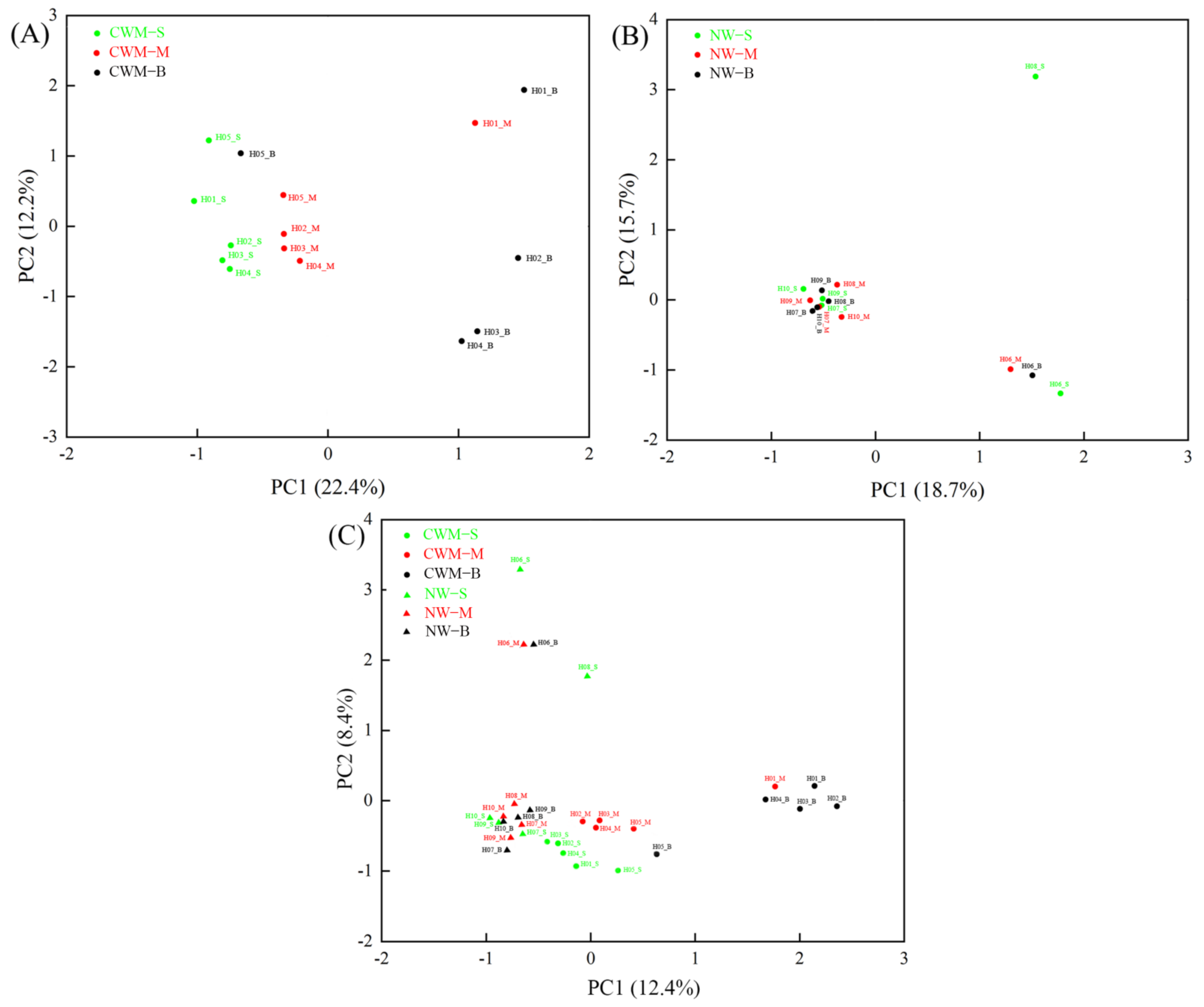
3.2. Structural Characteristics of the Eukaryotic Plankton Community

Analyzed by indices of richness and diversity at each CWM and NW sampling site, the eukaryotic plankton α-diversity of the groups varied greatly among all the samples. The total number of OTUs (2013 OTUs) in the CWM–B was the largest among the communities (Table 1). There was over 99% coverage of each sample library, fully reflecting the species and structure of the plankton community in the region. The Chao index indicates species richness, with higher values representing a greater total number of species. The CWM–B (Chao 2406) had the highest richness indices, which were significantly higher with respect to other samples. The OTUs and Chao indices of the surface, middle and bottom samples in the CWM were usually higher than NW and were significantly different from the Chao index of NW. The higher the Shannon diversity index, the more diverse the communities. The Shannon index indicated that the CWM–B (Shannon 5.40) exhibited the greatest species diversity, which was significantly different from the CWM–S diversity. However, the Simpson index was not significantly different in any sample. The mean number of OTUs per sample was 1650 and 712 for the CWM and NW, respectively, and the Simpson index was higher for the CWM than for NW. These results indicate that there was no significant difference in eukaryotic plankton diversity between the CWM and NW.

3.3. Changes in Composition and Diversity of Eukaryotic Plankton Community

Species annotation of the resulting OTUs sequences revealed that a total of 27 phyla, 98 classes, 243 orders, 379 families, 593 genera and 807 species of plankton were obtained. The number of eukaryotic species in CWM waters was 663 (distributed in 24 phyla), while the number of species in NW was 614 (distributed in 26 phyla). In the CWM, zooplankton, phytoplankton and fungi accounted for 89.45%, 9.77% and 0.78% of the total plankton, respectively; in NW, they accounted for 61.80%, 23.74% and 14.46% of the total plankton, respectively (Figure 2A). The relative abundance of zooplankton was the highest and the relative abundance of fungi was the lowest in CWM waters, consistent with NW. The taxonomic compositions of the eukaryotic plankton community varied dramatically. In general, a total of 24 and 26 phyla were detected in the CWM and NW eukaryotic plankton communities, respectively. The predominant phyla of the CWM and NW eukaryotic plankton communities included Arthropoda (66.27%, 44.91%), Cnidaria (15.48%, 3.21%), Bacillariophyta (4.83%, 16.72%), Chlorophyta (4.87%, 5.14%), Apicomplexa (3.49%, 8.47%) and Basidiomycota (0.38%, 12.19%), which accounted for 95.32% of the CWM sequences and 90.64% of the NW sequences. The relative abundance of Bacillariophyta and Basidiomycota in NW was much larger than that in the CWM, and the NW–S had the highest relative abundance (24.24%) for Basidiomycota, while the CWM–S had the lowest abundance (0.09%). The relative abundance of Cnidaria in the CWM was far from that in NW, and the CWM–S had the highest relative abundance (26.80%). Compared with the CWM–S and CWM–M, the CWM–B had a more even distribution of phyla (Figure 2B).
In this study, the main taxa of plankton were fungi, phytoplankton and zooplankton. The major classes (the top 10 classes with higher abundance) of these three taxa in the CWM and NW were analyzed (Figure 3). The predominant classes of the CWM and NW eukaryotic zooplankton communities included Copepoda (37.53%, 28.87%), Hydrozoa (8.64, 2.08%), Conoidasida (1.87%, 5.39%), Polycystinea (1.22%, 189%), Polychaeta (0.77%, 1.13%) and Ostracoda (0.13%, 0.29%). Appendicularia (0.80%), Tentaculata (0.19%) and Monogenea (0.4%) had a relatively large distribution in the CWM. Mammalia (0.38%) and Sagittoidea (0.33%) were mainly distributed in NW. In the CWM and NW, the eukaryotic phytoplankton communities mainly consisted of members of the classes Dinophyceae (33.34%, 29.88%), Coscinodiscophyceae (1.38%, 8.36%), Mamiellophyceae (1.08%, 2.08%), Haptophyceae (3.92%, 2.00%), Bacillariophyceae (0.64%, 1.31%), Mediophyceae (0.54%, 1.11%), Synurophyceae (0.53%, 0.53%) and Katablepharidophyta (0.66%, 0.28%). Pelagophyceae and Chloropicophyceae had a larger distribution in the CWM, accounting for 1.65% and 0.95%, respectively. Chrysophyceae (0.52%) and Dictyochophyceae (0.33%) were predominantly found in NW–M. From the distribution of different classes of fungi in the CWM and NW, the main classes found were Labyrinthulomycetes (0.44%, 0.66%), Dothideomycetes (0.03%, 0.66), Eurotiomycetes (0.07%, 0.61%), Agaricomycetes (0.18%, 0.35%), Oomycetes (0.03%, 0.30%), Tremellomycetes (0.01%, 0.13%), Basidiobolomycetes (0.02%, 0.08%) and Cystobasidiomycetes (0.01%, 0.08%). Chytridiomycetes (0.04%) and Malasseziomycetes (7.36%) were mainly found in the CWM and NW, respectively.
The dominant OTUs at the family level of each sample point in the CWM and NW were compared with each other (Figure 4). We found Malasseziaceae, Sarcocystidae, Skeletonemataceae, Harpacticidae, Cryptomonadaceae, Suessiaceae, Cymatosiraceae, Stephanodiscaceae and Miraciidae had greater relative abundance in NW than in the CWM. However, in the CWM, Chloropicaceae, Peridiniaceae, Phaeocystaceae, Katablepharidaceae, Warnowiaceae, Prymnesiaceae, Chrysochromulinaceae and Oikopleuridae showed higher relative abundance than in NW. Adeleidae, Plagoniidae, Glenodiniaceae and Stephanoecidae were predominantly found in the CWM–M and CWM–B, and the relative abundance of the CWM–B was greater than that of the CWM–M.
Eukaryotic plankton communities of the CWM and NW showed a clear pattern of specialization based on unweighted UniFrac distances with OTUs annotated at the genus level (PCA, Figure 5). The first and second PCA variations (22.4% for PC1 and 12.2% for PC2) accounted for a cumulative variance sum of 34.6% across all samples in the CWM (Figure 5A). On the PCA plot, the eukaryotic plankton communities from the CWM–S group, CWM–M group and CWM–M group were clustered separately, and the specialization of surface, middle and bottom in OTUs was unique to each water layer. All NW samples were clustered together, and there was no significant difference between the groups (Figure 5B). The statistical algorithms of Bray–Curtis were used to calculate the distance between the two samples and obtain the distance matrix. The heatmap was used to represent the distance matrix and observe the high and low distribution of the differences between the samples. Weighted and unweighted UniFrac distances showed the close proximity and some general differences of the eukaryotic plankton communities in the CWM group and NW group (Figure 6A,B). Disparity in the composition of eukaryotic plankton was presented in depths of different waters.
In summary, the results reveal that the microbial community profiles relatively differed and eukaryotic plankton communities could be significantly affected by different waters.

3.4. Environmental Factor Data Analysis

Environmental parameters of different water layers in the CWM and NW are shown in Table 2. The differences in waters’ effects on environmental characteristics indicate that water pH was slightly affected (p < 0.05) in both waters but the values remain non-significant under all samples. As the sampling depth increased, the salinity levels in the two waters increased, and the CWM group was significantly different from the NW group, with the maximum salinity level obtained from the CWM–B group. The water temperature varied greatly at different depths, with the CWM–B group having the lowest water temperature values (9.55 ± 0.28), which were all lower than that of other groups. It was also consistent with the characteristics of cold water masses. The highest levels of Chl a were in the CWM–S group (0.64 ± 0.03) and the lowest were in the CWM–B group (0.21 ± 0.04), with significant differences between the groups, and the highest levels of Chl a in NW were found in the NW–B group (1.41 ± 0.33). NW exhibited higher Chl a concentrations. The concentrations of NO2–N and NH4+−N in the five nutrient salts were stable and did not differ significantly between the two seas, and the content of NO3-N, PO43−-P and SiO32−-Si fluctuated considerably, among which the content of NO3-N, PO43−-P and SiO32−-Si in the CWM showed a trend of lowest at the surface and highest at the bottom.

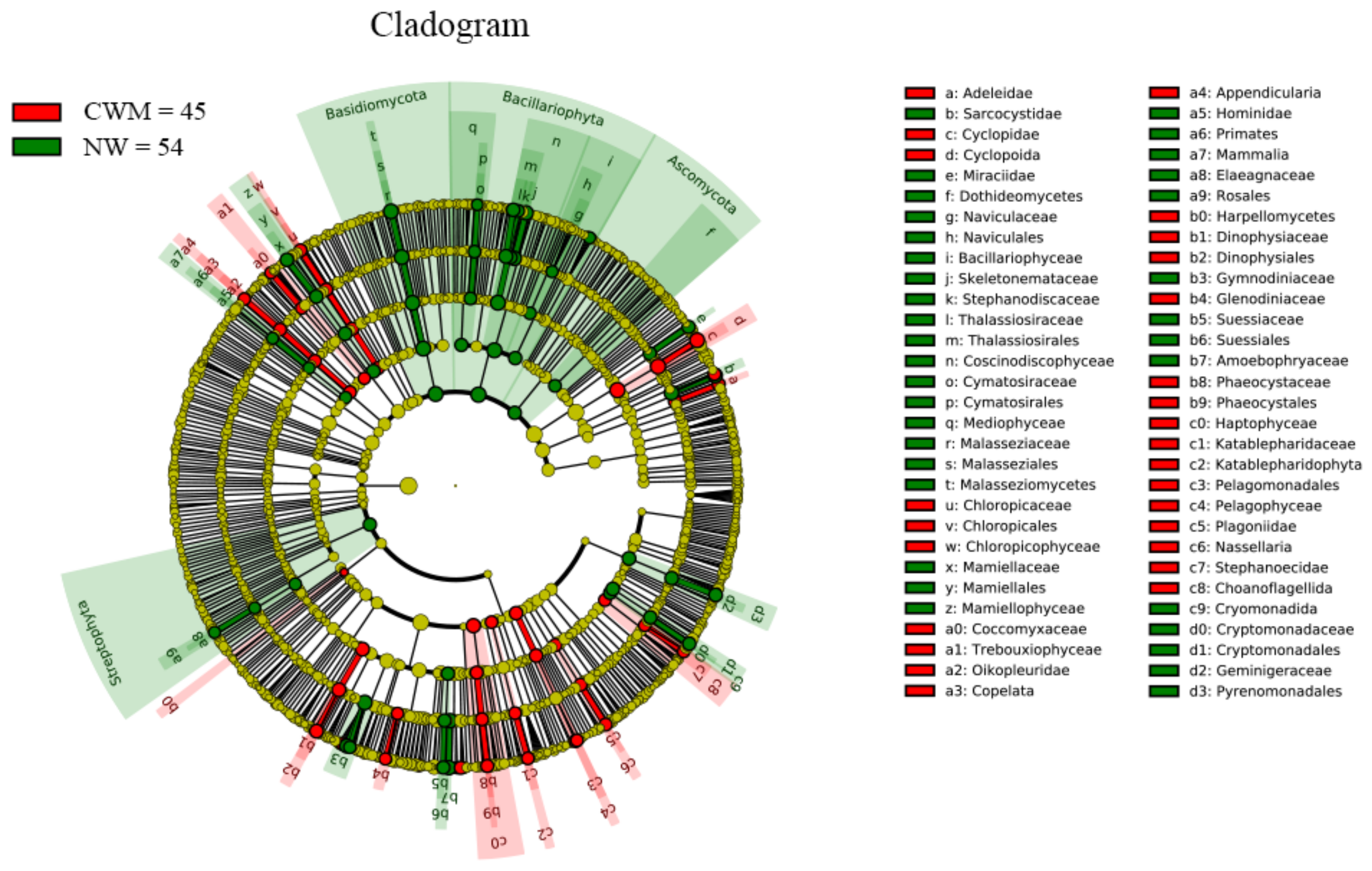
3.5. Comparative Assessment of Microbial Biomarkers

We used the non-parametric factorial Kruskal-Wallis (KW) sum-rank test to detect significant abundance difference characteristics and found taxa that were significantly different from abundance. Finally, we used the linear discriminant analysis effect size (LEfSe) method to estimate the magnitude of the effect of species abundance on differential effects and to further elucidate the possible interactions of the identified eukaryotic plankton affiliations in water samples. Through detecting the significant differences in the abundance of different eukaryotic plankton biomarkers in the detection group (linear discriminate analysis (LDA > 2; p < 0.05), the cladogram revealed that 99 biomarkers were identified in all water samples. Across all classification levels of the CWM−NW, 45 biomarkers were associated with the CWM and 54 were associated with the NW group (Figure 7). The higher abundance of Cyclopidae species (LDA 4.60, p = 0.02), including Cyclopoida and Eucyclops genera, was significantly enriched in the CWM group (Figure 7; Supplementary File S1). Bacillariophyta (LDA 4.54, p < 0.05) were highly abundant biomarkers identified in the NW group, and they consisted mainly of Thalassiosirales, Bacillariophyceae and Basidiomycota (LDA 4.42, p < 0.05), which were found to be significantly abundant in the NW group (Figure 7; Supplementary File S1).

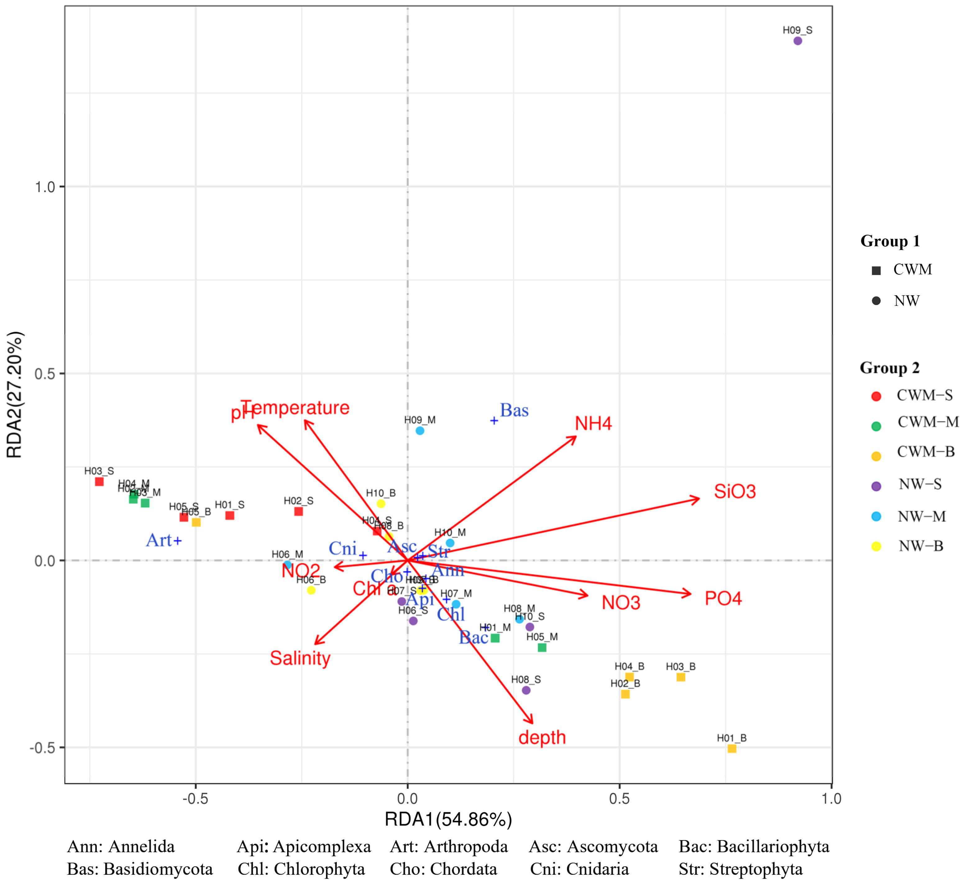
3.6. Correlation Analysis between Environmental Factors and Eukaryotic Planktonic Community Data

Redundancy analysis indicated relationships between environmental factors (water properties) and eukaryotic planktonic community composition, and results show that the relative abundance of eukaryotic plankton (Top 10) at the phylum level was affected by environmental properties (Figure 8). According to Figure 8, the first and second axes showed that 54.86% and 27.20% of changes in the eukaryotic plankton were influenced by water environmental properties. Depth was positively correlated with salinity, NO3-N, PO43-P, SiO32−-S, NH4+-N and Chl a in NW and negatively correlated with other environmental factors. The location of each sample on the RDA figure reflects the dependence of each species on different environmental resources. The significant abundance of Annelida, Apicomplexa, Bacillariophyta, Chlorophyta and Chordata was associated with water environmental indicators (NO2-N, NO3-N, PO43−-P, salinity, Chl a) and water depth. Basidiomycota is positively correlated with NH4+−N. Species abundance of Arthropoda and Cnidaria was significantly induced by pH in CWM waters. The slight change in SiO32−-S and NH4+-N levels was significantly associated with the change in Ascomycota and Streptophyta.

4. Discussion

High-throughput sequencing of environmental samples has the potential to detect rare, small and fragile species and has been shown to be feasible for biodiversity monitoring and quantification [33]. In this study, we used Illimina high-throughput sequencing technology to amplify the 18S rDNA V9 region DNA to explore the community structure of plankton in the South Yellow Sea, and we found that the number of reads in CWM waters was as high as 1,160,460 with 4006 OTUs; the number of reads in NW was 904,775 with 2591 OTUs. It can be seen that the OTUs of the Cold Water Mass in the South Yellow Sea are significantly higher than the nearshore waters of the South Yellow Sea. The species richness of eukaryotic plankton in the CWM was higher than that in NW, and the diversity was different but not significant. Therefore, we could divide the eukaryotic plankton into two relatively independent communities.
After smoothing the sample data, there were 326 phytoplankton species in NW, with a read count of 206,224 and fungal read count of 41,672, and 354 phytoplankton species in the CWM, with a read count of 188,036 and phytoplankton fungal read count of 4351. It was derived that although the total number of plankton was greater in the CWM than that in NW, the number of phytoplankton and planktonic fungi was higher in NW than that in the CWM. The reason lies in that the nutrient-rich salts brought to the nearshore waters by the freshwater discharged by the Yangtze River and the warm currents of the Yellow Sea provided favorable conditions for the growth of phytoplankton in the nearshore waters [34]. Dinophyceae with 115 species and Bacillariophyta with 73 species were the dominant phytoplankton groups in this area, while Prorocentrum 14.83%, Gymnodiniaceae 12.35% and Skeletonema 7.89% were the dominant species. As described in previous reports [35], which analyzed the species composition and distribution characteristics of phytoplankton in the Yellow Sea in spring and autumn using microscopic methods, phytoplankton were mainly Bacillariophyta and Dinophyta. During autumn and winter, the wind speed above the NW increases and is influenced by freshwater runoff into the sea, and Bacillariophyta and Dinophyta are protected by a silicified cell wall that can persist during strong current turbulence, providing the main support for phytoplankton biomass in the NW [36]. Skeletonema was a major red tide bacillariophyta in China’s coastal waters, posing a direct threat to marine aquaculture, aquatic food safety and ecosystem health, and its favorable growth temperature is 25 °C [37]. The NW provide a suitable growth temperature for it. Similarly, nearshore eutrophication was a necessary trigger for Bacillariophyta water blooms and occurrence [38]. The NW area was small and shallow, and the total number of plankton samples was lower. At the same time, small-scale coastal waters were significantly influenced by anthropogenic activities, and environmental variability was more likely to cause dramatic changes in the plankton community [39]. Moreover, phytoplankton compete for survival in the water. The high abundance of dominant species of Dinophyta and Bacillariophyta inhibits the growth of other phytoplankton, increases the polarization of numbers between communities, decreases uniformity and was an important cause leading to low phytoplankton diversity. The eukaryotic zooplankton assemblages in NW consisted mainly of Arthropoda, Apicomplexa and Cnidaria, and the dominant genera were Neocalanus, Besnoitia, Acanthocyclops and Muggiaea. The results obtained from the study are consistent with the distribution area [40]. Due to the differences in temperature and salinity tolerance among zooplankton, the species composition and abundance of zooplankton vary, thus affecting their community structure [41]. Neocalanus, as the dominant species, was a wide-temperature, wide-saline species, whose development and growth depend on temperature, and whose embryonic development has an upper temperature tolerance of 23 °C [42], making it one of the dominant species of coastal zooplankton in China. However, due to predation by other organisms, it results in lower abundance of Neocalanus in NW than that in the CWM from summer to fall [43]. Among them, Muggiaea secretes toxins during growth that can bind to nets and cause depletion of nearshore marine fishery resources [44]. Temperature and dissolved organic matter were two important factors in the regulation of fungal productivity. Within a certain temperature range, the increase in temperature helped the fungus to metabolize and increase its productivity. Fungal productivity was usually consistent with the trend in the distribution of Chl a content and also higher in marine areas with higher Chl a content [45]. Seawater temperature was stable and Chl a was abundant in the NW of this study (Table 2). The Yangtze River brings large amounts of freshwater into the ecosystem, and the use of nitrogen fertilizers in agricultural practices in the Yangtze River basin leads to increased concentrations of nitrogen and phosphorus (Table 2) [46,47]. Therefore, Basidiomycota and Ascomycota mainly dominate the NW, with Malassezia being the dominant genus, accounting for 67.46% of the total amount of pelagic fungi. The fungal species obtained by Zhang Li et al. based on ITS region amplification were also dominated by Basidiomycota [48]. The dissolved organic matter released by jellyfish usually had a high carbon to nitrogen ratio, which facilitates fungal respiration [49,50]. Previous studies found that rapid phytoplankton growth can limit fungal productivity. Station H_09 had fewer phytoplankton than other stations, so Malassezia was mainly clustered at this station.
Historical studies show that zooplankton abundance in the South Yellow Sea in autumn reveals a gradual increase from the nearshore to the central sea [51]. The abundance and biomass of zooplankton distributed in CWM waters were generally high, and Gao et al. also showed that salinity was one of the most important environmental factors affecting the zooplankton community characteristics in the Yangtze estuary [52]. The CWM was not susceptible to nearshore anthropogenic factors, had relatively high salinity (Table 2) and provided a stable habitat for most zooplankton, and the colder temperatures of the Cold Water Mass allow it to escape high-temperature damage. Therefore, Neocalanus, Eucyclops, Acanthocyclops and Muggiaea in Arthropoda and Cnidaria were the most dominant zooplankton in the CWM of the South Yellow Sea, accounting for 41.63%, 11.94%, 8.19% and 15.52% of the total zooplankton, respectively. Neocalanus and Acanthocyclops had a wide range of temperature tolerance, but there were some limitations. Liang and Uye found that Neocalanus was present year-round in Fukuyama Port, Japan, but the growth rate no longer increases at water temperatures above 20 °C [53]. For photosynthetic autotrophic plankton, the most suitable environment was the thermocline. Due to the stratification phenomenon, the upper layer of seawater had the advantage of light and temperature, while the deeper layer had a higher concentration of nutrients, low light, low temperature and other extreme environmental conditions, resulting in significant differences in species diversity (Table 1). In the thermocline, the temperature changes quickly, and the temperature drops from about 23 to 8 °C at a vertical distance of about 20 m. The mixing of cold and warm water is accompanied by nutrient salts and other life elements, which provides favorable conditions for the mass reproduction of photosynthetic autotrophs. This was one of the reasons why zooplankton were more abundant in the CWM waters than in NW. Eukaryotic algae with smaller particle sizes in seawater are generally more abundant in oceans far away from nearshore waters, thus increasing phytoplankton diversity in cold water masses and providing a good food base for zooplankton [54]. Predation on microscopic phytoplankton by large numbers of zooplankton in CWM waters exacerbates zooplankton growth and reproduction. The dominant eukaryotic phytoplankton species in the CWM waters were similar to those in the NW and were also dominated by Dinophyceae (119 species). Among them, Prorocentrum was the dominant species, accounting for 23.63% of the total number of phytoplankton. Bacillariophyta were less abundant in the CWM compared to the NW, with Skeletonema accounting for only 0.30% of the total phytoplankton. Li et al. found that the phosphate concentration was low and the growth of Skeletonema may be affected, whereas this may facilitate the growth of Prorocentrum [55]. A previous study also reported that during the autumn season, bacillariophyta correlated with the silicate concentration [56]. Therefore, it can be assumed that silicate was the important controlling factor. The SiO32−-Si content in the CWM was smaller than that in the NW and was only abundantly distributed at the bottom of the Cold Water Mass, so the Bacillariophyta abundance was relatively small. It had been explained in previous studies that water depth may impact the abundance of phytoplankton distribution as the nutrient concentrations increased vertically because of sinking [57,58]. The CWM had a higher water depth than NW, and nutrient salt concentrations were deposited, providing favorable conditions for phytoplankton diversity. Although the temperature decreases with depth, Dinophyta can be protected by a thick cell wall of cellulose and thus grow well. For the fungi in the CWM, the upper layer of water had a suitable growth temperature and light, but the concentration of nutrient salts was low, and the deep layer had deposited nutrient salts but low temperature and low light, so there was a lower number of fungi. Malassezia accounted for only 0.62% of the total plankton, while Thraustochytrium, the dominant genus, accounted for only 10.99% of the total plankton. Shiah and Ducklow suggested that the distribution of fungi was synergistically influenced by three factors: temperature, nutrient salt supply (bottom-up control) and feeding pressure (top-down control) [59]. The lower temperature in the Cold Water Mass and the large amount of zooplankton feeding brought differences in the fungal community in the spatial distribution pattern.
It was found that the plankton in different waters varied widely in species abundance and diversity. NW were subject to freshwater impacts and anthropogenic influences in the Yangtze River, and the area had high nutrient salt concentrations that provide a good habitat for phytoplankton. Previous studies also showed that a higher Chl a content gives the South Yellow Sea high primary productivity in spring and autumn [60]. NW generally have a higher Chl a content (Table 2), so the region is rich in phytoplankton biomass. However, the depth of seawater in the NW area was shallow, and due to the strong winds associated with Typhoon Hibei-Shi, the seawater in each layer was easily mixed with sediment, which affects the growth of plankton; therefore, it can be seen from Table 2 and Figure 5 and Figure 6 that there was no significant difference in nutrient salts in the water samples of each layer, and the plankton species are also concentrated. Other important factors were the CWM’s distance from the coast and the peculiar stratification that provide a good and stable habitat for zooplankton. It was also known from this study that the zooplankton species richness was higher in CWM waters than that in NW due to the influence of the food chain and the role of zooplankton as predators in the plankton food chain on microscopic phytoplankton predation in CWM waters. Therefore, this also causes the phytoplankton biomass to be lower. At the same time, the vertical transport of nutrient salt by a continuous and stable upwelling system in CWM waters can further promote biological activity in the upper water column [61], which can also apparently provide additional assurance of sea-derived material for the deposition of biological residues and their nutrients to the bottom.
As shown by RDA analysis (Figure 8), significant changes in water environmental factors were likely associated with changes in plankton community composition and diversity. Depth was positively correlated with NO3-N, PO43−-P, SiO32−-S, salinity and Chl a. An increase in water depth caused a vertical increase in nutrient deposition, and depth had a strong influence on plankton distribution. Most of the zooplankton biomass and abundance in this study were positively correlated with water depth. Tavernini et al. also found that water depth was strongly correlated with zooplankton community structure [62]. There was a negative correlation between temperature and water depth, with a decrease in the number of Arthropoda and Cnidaria as depth increased and water temperature decreased, indicating that salinity had a stronger effect on these two species than water temperature had. Additionally, as broad-temperature, broad-salt species, they had a strong positive correlation with nitrite, Chl a and salinity. Algae are required as primary producers for photosynthesis, which, in turn, require nitrogen and phosphorus, which are required as basic nutrients. In this study, nitrogen and phosphorus levels had a significant impact on the phytoplankton community. Le et al. showed that high concentrations of ammonium support higher cell abundance in phytoplankton, and our RDA analysis yielded the same results [63]. Depth, salinity and Chl a showed significant positive correlations with Apicomplexa and Chordata. Annelida, Bacillariophyta and Chlorophyta are strongly correlated with depth, NO3-N, PO43−-P and SiO32−-S. Similarly, our analysis showed that nitrate concentration had a strong effect on the abundance of phytoplankton. Thus, we found that phytoplankton abundance in NW was higher than in the CWM, the reason of which may be the variation in nutrient salt concentration between these two regions (Table 2). Increased rainfall and river inflows during the autumn increased nitrate and silicate levels in the water column. An increase in nitrate and phosphate also increases Bacillariophyta proliferation and eventually leads to the accumulation of silicates in the sediment [64]. Such an environment also contributes to the growth of Annelida. In our study, CWM silicate concentrations were lower than NW, which may account for the increased abundance of Dinophyta and decreased abundance of Bacillariophyta in the CWM.
The high-throughput sequencing technology based on 18S rDNA has high work efficiency, but it also has some disadvantages. First, quantitative DNA extraction may be affected by heterogeneity in cell wall stability. Furthermore, rDNA copy number variation affects the relative abundance estimates of all species in the sample. In addition, the number of resting stages varies among samples [65]. At the same time, the loss of cells in preserved samples can also lead to observed differences in species abundance. If the cell losses are taxon-specific and differ between species, they can bias the relative taxon abundances in the morphological samples [66]. Therefore, the combination of high-throughput sequencing technology and morphological observation can conduct a more comprehensive study on the community distribution of plankton.

5. Conclusions

High-throughput sequencing technology based on 18S rDNA can obtain a richer number of zooplankton, phytoplankton and fungi. The relative abundance of zooplankton was the highest and the relative abundance of fungi was the lowest in CWM waters, consistent with NW. Dinophyta and Bacillariophyta were the most abundant phyla of phytoplankton in the two areas. Arthropoda and Cnidaria were the major zooplankton taxa. The dominant fungal population was mainly Basidiomycota. Total plankton abundance was highest in CWM waters. However, the number of phytoplankton and fungal reads in NW was higher than that in cold water masses. The NW were the main source of dissolved nutrients affecting the phytoplankton community. Ammonium salts, nitrates, phosphates, silicates and water depth were important factors affecting phytoplankton growth. Depth and microscopic phytoplankton were important factors influencing the structure of the zooplankton community. Meanwhile, high-throughput sequencing is a new method for plankton research, and this study adopts this method from the side to reflect the diversity of eukaryotic plankton in the South Yellow Sea and its relationship with the environment; however, every research method is not all-powerful, and the high-throughput sequencing method is also limited by the database used. Hence, it can be combined with traditional microscopy methods to conduct a more comprehensive and in-depth study in this field. Many of the conclusions in the paper corroborate the patterns obtained by previous traditional methods, and some of the different conclusions from the previous ones await further research. Therefore, long-term integrated plankton observations are needed to better understand the combined effects of physicochemical and biological factors on marine ecology.

Supplementary Materials

The following are available online at https://0-www-mdpi-com.brum.beds.ac.uk/1424-2818/13/1/21/s1, Table S1: Summary of 18S rDNA read counts for all samples, Figure S1: Shannon rarefaction curves for all samples, Figure S2: OTU Venn analysis of all samples, Supplementary File S1: Community composition of the CWM and NW.

Author Contributions

Conceptualization, J.S. and Y.S..; methodology, C.W., X.F. and L.L.; software, Y.S., Y.L., L.L. and C.G.; formal analysis, Y.S., C.W.; writing—original draft preparation, Y.S., J.S. and Y.L.; supervision, J.S., Y.S., C.W., C.G. and Y.L.; project administration, J.S.; funding acquisition, J.S. All authors have read and agreed to the published version of the manuscript.

Funding

This work was jointly supported by the following research grants awarded to Professor Jun Sun: the National Nature Science Foundation of China (41876134, 41676112 and 41276124), the University Innovation Team Training Program for Tianjin (TD12-5003), the Tianjin 131 Innovation Team Program (20180314) and the Changjiang Scholar Program of Chinese Ministry of Education (T2014253).

Institutional Review Board Statement

Not applicable.

Informed Consent Statement

Informed consent was obtained from all subjects involved in the study.

Data Availability Statement

The data presented in this study are openly available in NCBI at PRJNA664010. (https://dataview.ncbi.nlm.nih.gov/object/PRJNA664010)

Conflicts of Interest

The authors declare no conflict of interest.

References

  1. Bigg, G.R.; Jickells, T.D.; Liss, P.S.; Osborn, T.J. The role of the oceans in climate. Int. J. Climatol. 2003, 23, 1127–1159. [Google Scholar] [CrossRef]
  2. Tatiana, A.R.; Ellen, O.L.; Virginia, A.E. Metapopulation structure in the planktonic diatom ditylum brightwellii (Bacillariophyceae). Protist 2009, 160, 111–121. [Google Scholar] [CrossRef]
  3. Gao, H.; Zhang, S.; Zhao, R.; Zhu, L. Plankton community structure analysis and water quality bioassessment in Jiulong Lake. IOP Conf. Ser. Earth Environ. Sci. 2018, 199, 022031. [Google Scholar] [CrossRef]
  4. Yuan, M.; Zhang, C.; Jiang, Z.; Guo, S.; Sun, J. Seasonal variations in phytoplankton community structure in the Sanggou, Ailian, and Lidao Bays. J. Ocean Univ. China 2014, 13, 1012–1024. [Google Scholar] [CrossRef]
  5. Eiler, A.; Drakare, S.; Bertilsson, S.; Pernthaler, J.; Peura, S.; Rofner, C.; Lindström, E.S. Unveiling distribution patterns of freshwater phytoplankton by a next generation sequencing based approach. PLoS ONE 2013, 8, e53516. [Google Scholar] [CrossRef]
  6. Bianchi, F.; Acri, F.; Aubry, F.B.; Berton, A.; Boldrin, A.; Camatti, E.; Comaschi, A. Can plankton communities be considered as bio-indicators of water quality in the Lagoon of Venice? Mar. Pollut. Bull. 2003, 46, 964–971. [Google Scholar] [CrossRef]
  7. Li, Q.; Zhao, Y.; Zhang, X.; Wei, Y.; Qiu, L.; Wei, Z.; Li, F. Spatial heterogeneity in a deep artificial lake plankton community revealed by PCR-DGGE fingerprinting. Chin. J. Oceanol. Limnol. 2015, 33, 624–635. [Google Scholar] [CrossRef]
  8. Sun, J. Marinephytolankton and biological carbon sink. Acta Ecol. Sin. 2011, 31, 5372–5378. [Google Scholar]
  9. Charlson, R.J.; Lovelock, J.E.; Andreae, M.O.; Warren, S.G. Oceanic phytoplankton, atmospheric sulphur, cloud albedo and climate. Nature 1987, 326, 655–661. [Google Scholar] [CrossRef]
  10. Sathyendranath, S.; Gouveia, A.D.; Shetye, S.R. Biological control of surface temperature in the Arabian Sea. Nature 1991, 349, 54–56. [Google Scholar] [CrossRef]
  11. Sun, J. Geometric models for calculating cell biovolume and surface area for phytoplankton. J. Plankton Res. 2003, 25, 1331–1346. [Google Scholar] [CrossRef] [Green Version]
  12. Silva, C.A.D.; Train, S.; Rodrigues, L.C. Phytoplankton assemblages in a Brazilian subtropical cascading reservoir system. Hydrobiologia 2005, 537, 99–109. [Google Scholar] [CrossRef]
  13. Warwick, R.M. The nematode/copepod ratio and its use in pollution ecology. Mar. Pollut. Bull. 1981, 12, 329–333. [Google Scholar] [CrossRef]
  14. Goh, T.K.; Hyde, K.D. Biodiversity of freshwater fungi. J. Ind. Microbiol. 1996, 17, 328–345. [Google Scholar] [CrossRef]
  15. Cudowski, A.; Pietryczuk, A.; Hauschild, T. Aquatic fungi in relation to the physical and chemical parameters of water quality in the Augustów Canal. Fungal Ecol. 2015, 13, 193–204. [Google Scholar] [CrossRef]
  16. Xiao, X.; Sogge, H.; Lagesen, K.; Tooming, K.A.; Jakobsen, K.S.; Rohrlack, T. Use of high throughput sequencing and light microscopy show contrasting results in a study of phytoplankton occurrence in a freshwater environment. PLoS ONE 2014, 9, e106510. [Google Scholar] [CrossRef] [PubMed]
  17. Mitchell, L.S.; Hilary, G.M.; Julie, A.H.; David, M.W.; Susan, M.H.; Phillip, R.N.; Jesus, M.A.; Gerhard, J.H. Microbial diversity in the deep sea and the underexplored “Rare Biosphere”. Proc. Natl. Acad. Sci. USA 2006, 103, 12115–12120. [Google Scholar] [CrossRef] [Green Version]
  18. Bucklin, A.; Frost, B.; Bradford, G.J.; Allen, L.; Copley, N. Molecular systematic and phylogenetic assessment of 34 calanoid copepod species of the Calanidae and Clausocalanidae. Mar. Biol. 2003, 142, 333–343. [Google Scholar] [CrossRef]
  19. Behnke, A.; Engel, M.; Christen, R.; Nebel, M.; Klein, R.R.; Stoeck, T. Depicting more accurate pictures of protistan community complexity using pyrosequencing of hypervariable SSU rRNA gene regions. Environ. Microbiol. 2010, 13, 340–349. [Google Scholar] [CrossRef]
  20. De Vargas, C.; Audic, S.; Henry, N.; Decelle, J.; Mahe, F.; Logares, R.; Lara, E.; Berney, C.; Le Bescot, N.; Probert, I.; et al. Eukaryotic plankton diversity in the sunlit ocean. Science 2015, 348, 1261605. [Google Scholar] [CrossRef] [Green Version]
  21. Zou, E.M.; Guo, B.H.; Tang, Y.X.; Lee, J.H.; Xiong, X.J.; Zeng, X.M. The hydrographic features and mixture and exchange of sea water in the southern Huanghai Sea in autumn. Acta Oceanol. Sinca 1999, 21, 12–21. [Google Scholar] [CrossRef]
  22. Xia, C.; Qiao, F.; Yang, Y.; Ma, J.; Yuan, Y. Three-dimensional structure of the summertime circulation in the Yellow Sea from a wave-tide-circulation coupled model. J. Geophys. Res. 2006, 111. [Google Scholar] [CrossRef]
  23. Lü, X.; Qiao, F.; Xia, C.; Wang, G.; Yuan, Y. Upwelling and surface cold patches in the Yellow Sea in summer: Effects of tidal mixing on the vertical circulation. Cont. Shelf Res. 2010, 30, 620–632. [Google Scholar] [CrossRef]
  24. Sun, S.; Wang, R.; Zhang, G.T.; Yang, P.; Zhang, F. A preliminary study on the over-summer strategy of Calanus Sinicus in the Yellow Sea. Oceanol. Limnol. Sinica 2002, 92–99. [Google Scholar]
  25. Oh, K.H.; Lee, S.; Song, K.M.; Lie, H.J.; Kim, Y.T. The temporal and spatial variability of the Yellow Sea Cold Water Mass in the southeastern Yellow Sea, 2009–2011. Acta Oceanol. Sin. 2013, 32, 1–10. [Google Scholar] [CrossRef]
  26. Jeffrey, S.W.; Humphrey, G.F. New spectrophotometric equations for determining chlorophylls a, b, c1 and c2 in higher plants, algae and natural phytoplankton. Biochem. und Physiol. der Pflanz. 1975, 167, 191–194. [Google Scholar] [CrossRef]
  27. Yuan, J.; Li, M.; Lin, S. An Improved DNA Extraction method for efficient and quantitative recovery of phytoplankton diversity in natural assemblages. PLoS ONE 2015, 10, e0133060. [Google Scholar] [CrossRef]
  28. Maral-Zettler, L.A.; McCliment, E.A.; Ducklow, H.W.; Huse, S.M.; Langsley, G. A Method for Studying Protistan Diversity Using Massively Parallel Sequencing of V9 Hypervariable Regions of Small-Subunit Ribosomal RNA Genes. PLoS ONE 2009, 4, e6372. [Google Scholar] [CrossRef]
  29. Huse, S.M.; Welch, D.M.; Morrison, H.G.; Sogin, M.L. Ironing out the wrinkles in the rare biosphere through improved OTU clustering. Environ. Microbiol. 2010, 12, 1889–1898. [Google Scholar] [CrossRef] [Green Version]
  30. Bokulich, N.A.; Subramanian, S.; Faith, J.J.; Gevers, D.; Gordon, J.I.; Knight, R. Quality-filtering vastly improves diversity estimates from Illumina amplicon sequencing. Nat. Methods 2013, 10, 57–59. [Google Scholar] [CrossRef]
  31. Schloss, P.D.; Westcott, S.L.; Ryabin, T.; Hall, J.R.; Hartmann, M.; Hollister, E.B. Introducing mothur: Open-source, platform-independent, community-supported software for describing and comparing microbial communities. Appl. Environ. Microbiol. 2009, 75, 7537–7541. [Google Scholar] [CrossRef] [PubMed] [Green Version]
  32. Sheik, C.S.; Mitchell, T.W.; Rizvi, F.Z.; Rehman, Y.; Faisal, M.; Hasnain, S.; Krumholz, L.R. Exposure of soil microbial communities to chromium and arsenic alters their diversity and structure. PLoS ONE 2010, 7, e40059. [Google Scholar] [CrossRef] [PubMed]
  33. Hajibabaei, M.; Shokralla, S.; Zhou, X.; Singer, G.A.C.; Baird, D.J. Environmental barcoding: A next-generation sequencing approach for biomonitoring applications using river benthos. PLoS ONE 2011, 6, e17497. [Google Scholar] [CrossRef] [PubMed] [Green Version]
  34. Wang, X.D.; Li, C.L. Classification of zooplankton communities in the adjacent waters of the Changjiang River estuary based on data from 1998 to 2011. Mar. Sci. 2018, 42, 38–47. [Google Scholar] [CrossRef]
  35. Liu, L.H. The Community Structure and Diversity Analysis of Phytoplankton in the Yellow Sea and the Chang Jiang Estuary Waters. Ph.D. Thesis, Ocean University of China, Shandong, China, 2007. (In Chinese). [Google Scholar] [CrossRef]
  36. Hamm, C.E.; Merkel, R.; Springer, O.; Jurkojc, P.; Maier, C.; Prechtel, K.; Smetacek, V. Architecture and material properties of diatom shells provide effective mechanical protection. Nature 2003, 421, 841–843. [Google Scholar] [CrossRef] [Green Version]
  37. Li, X.; Yan, T.; Lin, J.; Yu, R.; Zhou, M. Detrimental impacts of the dinoflagellate Karenia mikimotoi in Fujian coastal waters on typical marine organisms. Harmful Algae 2017, 61, 1–12. [Google Scholar] [CrossRef]
  38. Tang, D.L.; Ni, I.H.; MüllerKarger, F.E.; Liu, Z.J. Analysis of annual and spatial patterns of CZCS-derived pigment concentration on the continental shelf of China. Cont. Shelf Res. 1998, 18, 1493–1515. [Google Scholar] [CrossRef]
  39. Ning, X.X.; Ji, L.; Wang, G.; Xia, B.X. Phytoplankton community in the nearshore waters of Laizhou Bay in 2009. Trans. Oceanol. Limnol. 2011, 3, 97–104. [Google Scholar] [CrossRef]
  40. Zuo, T.; Wang, R.; Chen, Y.Z.; Gao, S.W.; Wang, K. Net macro-zooplankton community classification on the shelf area of the East China Sea and the Yellow Sea in spring and autumn. Acta Ecol. Sin. 2005, 25. [Google Scholar] [CrossRef]
  41. Zheng, Z.; Li, S.; Xu, Z. Marine Zooplankton Biology; China Ocean Press: Beijing, China, 1984; pp. 139–491. [Google Scholar]
  42. Uye, S. Temperature-dependent development and growth of Calanus sinicus (Copepoda: Calanoida) in the laboratory. Hydrobiologia 1988, 167, 285–293. [Google Scholar] [CrossRef]
  43. Huo, Y.Z. Study on the Zooplankton Functional Groups in the Yellow Sea. Ph.D. Thesis, Graduate University of Chinese Academy of Sciences, Shandong, China, 2008. (In Chinese). [Google Scholar]
  44. Jiang, H.; Cheng, H.Q.; Xu, H.G.; Arreguín, S.F.; Zetina, R.M.J.; Del, M.L.P.; Le, Q.W.J.F. Trophic controls of jellyfish blooms and links with fisheries in the East China Sea. Ecol. Model. 2008, 212, 492–503. [Google Scholar] [CrossRef]
  45. Yuan, X.C.; Yin, K.D.; Harrison, P.J. Bacterial production and respiration in subtropical Hong Kong waters: Influence of the Pearl River discharge and sewage effluent. Aquat. Microb. Ecol. 2010, 58, 167–179. [Google Scholar] [CrossRef] [Green Version]
  46. Chao, S.Y. Circulation of the East China Sea, a numerical study. J. Oceanogr. 1990, 46, 273–295. [Google Scholar] [CrossRef]
  47. Li, M.; Xu, K.; Watanabe, M.; Chen, Z. Long-term variations in dissolved silicate, nitrogen, and phosphorus flux from the Yangtze River into the East China Sea and impacts on estuarine ecosystem. Estuar. Coast. Shelf Sci. 2007, 71, 3–12. [Google Scholar] [CrossRef]
  48. Zhang, L.; Lin, J.N.; Zhang, Y.; Wang, A.P. Eukaryotic micro-plankton community diversity and characteristics of regional distribution in the Yellow Sea by ITS high-throughput sequencing. Environ. Scince 2018, 39, 2368–2379. [Google Scholar] [CrossRef]
  49. Condon, R.H.; Steinberg, D.K.; Del, P.A.; Bouvier, T.C.; Bronk, D.A.; Graham, W.M.; Ducklow, H.W. Jellyfish blooms result in a major microbial respiratory sink of carbon in marine systems. Proc. Natl. Acad. Sci. USA 2011, 108, 10225–10230. [Google Scholar] [CrossRef] [Green Version]
  50. Niggl, W.; Naumann, M.S.; Struck, U.; Manasrah, R.; Wild, C. Organic matter release by the benthic upside-down jellyfish Cassiopea sp. fuels pelagic food webs in coral reefs. J. Exp. Mar. Biol. Ecol. 2010, 384, 99–106. [Google Scholar] [CrossRef]
  51. Chen, X.C.; Huang, Y.; Mu, X.Y.; Zhu, L.Y.; Pu, Y.Q. Distribution characteristics of zooplankton in the Southern Yellow Sea in summer and winter. Period. Ocean Univ. China 2018, 48, 50–56. [Google Scholar]
  52. Gao, Q.; Xu, Z.; Zhuang, P. The relation between distribution of zooplankton and salinity in the Changjiang Estuary. Chin. J. Oceanol. Limnol. 2008, 26, 178–185. [Google Scholar] [CrossRef]
  53. Liang, D.; Uye, S. Population dynamics and production of the planktonic copepods in a eutrophic inlet of the Inland Sea of Japan. III. Paracalanus sp. Mar. Biol. 1996, 127, 219–227. [Google Scholar] [CrossRef]
  54. Wang, H.L.; Huang, B.Q.; Hong, H.S. Size-fractionated productivity and nutrient dynamics of phytoplankton in subtropical coastal environments. Hydrobiologia 1997, 352, 97–106. [Google Scholar] [CrossRef]
  55. Li, R.X.; Zhu, M.Y.; Wang, Z.L.; Shi, X.Y.; Chen, B.Z. Mesocosm experiment on competition between two HAB species in East China Sea. Chin. J. Appl. Ecol. 2003, 14, 1049–1054. [Google Scholar]
  56. Guo, S.; Feng, Y.; Wang, L.; Dai, M.; Liu, Z.; Bai, Y.; Sun, J. Seasonal variation in the phytoplankton community of a continental-shelf sea: The East China Sea. Mar. Ecol. Prog. 2014, 516, 103–126. [Google Scholar] [CrossRef] [Green Version]
  57. De Queiroz, A.R.; Flores Montes, M.; De Castro Melo, P.A.M.; Da Silva, R.A.; Koening, M.L. Vertical and horizontal distribution of phytoplankton around an oceanic archipelago of the Equatorial Atlantic. Mar. Biodivers. Rec. 2015, 8. [Google Scholar] [CrossRef]
  58. Wei, N.; Satheeswaran, T.; Jenkinson, I.R.; Xue, B.; Wei, Y.; Liu, H.; Sun, J. Factors driving the spatiotemporal variability in phytoplankton in the Northern South China Sea. Cont. Shelf Res. 2018, 162, 48–55. [Google Scholar] [CrossRef]
  59. Shiah, F.K.; Ducklow, H.W. Temperature regulation of heterotrophic bacterioplankton abundance, production, and specific growth rate in Chesapeake Bay. Limnol. Oceanogr. 1994, 39, 1243–1258. [Google Scholar] [CrossRef]
  60. Song, J.M. Biogeochemistry of China Marginal Seas; Shandong Science and Technology Press: Jinan, China, 2004. [Google Scholar]
  61. Pang, C.G.; Hu, D.X. Upwelling and sedimentation dynamics III: Coincidence of upwelling areas with mud patches in north hemisphere shelf seas. Chin. J. Oceanol. Limnol. 2002, 20, 101–106. [Google Scholar] [CrossRef]
  62. Tavernini, S.; Mura, G.; Rossetti, G. Factors Influencing the Seasonal Phenology and Composition of Zooplankton Communities in Mountain Temporary Pools. Int. Rev. Hydrobiol. 2005, 90, 358–375. [Google Scholar] [CrossRef]
  63. Le, F.; Sun, J.; Ning, X.; Song, S.; Cai, Y.; Liu, C. Phytoplankton in the northern south China sea in summer 2004. Oceanol. Limnol. Sin. 2006, 37, 238. [Google Scholar] [CrossRef]
  64. Conley, D.J.; Schelske, C.L.; Stoermer, E.F. Modification of the biogeochemical cycle of silica with eutrophication. Mar. Ecol. Prog. Ser. 1993, 101, 179–192. [Google Scholar] [CrossRef]
  65. Medinger, R.; Nolte, V.; Pandey, R.V.; Jost, S.; Ottenwalder, B.; Schlotterer, C.; Boenigk, J. Diversity in a hidden world: Potential and limitation of next-generation sequencing for surveys of molecular diversity of eukaryotic microorganisms. Mol. Ecol. 2010, 19, 32–40. [Google Scholar] [CrossRef] [PubMed] [Green Version]
  66. Sime, N.T.; Grolière, C.A. Effets quantitatifs des fixateurs sur le stockage des ciliés d’eaux douces. Archiv. Protistenkd. 1991, 140, 109–120. [Google Scholar]
Figure 1. Location of sampling sites in the South Yellow Sea.
Diversity 13 00021 g001
Figure 2. UniFrac UPGMA (unweighted pair group method with arithmetic mean) clustering analysis revealed the dominant plankton kingdoms (A) and phyla (B) in all samples from different waters of the South Yellow Sea. Cold Water Mass populations (CWM: all; CWM–S: surface; CWM–M: middle; CWM–B: bottom); nearshore waters populations (NW: all; NW–S: surface; NW–M: middle; NW–B: bottom).
Diversity 13 00021 g002
Figure 3. Circos figure revealing the ten zooplankton, phytoplankton and fungi with the highest relative abundance among the classes in different waters of the South Yellow Sea. (CWM: Cold Water Mass; NW: nearshore waters; F: fungi; P: phytoplankton; Z: zooplankton).
Diversity 13 00021 g003
Figure 4. Unweighted pair group method with arithmetic mean (UPGMA) and heatmap of eukaryotic plankton families with relative abundances across different samples. Colors indicate taxa with a higher (red) or lower (blue) relative abundance in each sample. Cold Water Mass (CWM) populations (H01_S–H05_S: surface; H01_M–H05_M: middle; H01_B–H05_B: bottom); nearshore waters (NW) populations (H06_S–H10_S: surface; H06_M–H10_M: middle; H06_B–H10_B: bottom).
Diversity 13 00021 g004
Figure 5. Principal component analysis (PCA) of eukaryotic plankton communities (genus level) according to the two populations (CWM and NW). Taxonomic (OTU) clustering based on unweighted UniFrac distances. (A): Principal component analysis of eukaryotic plankton communities in the CWM; (B): Principal component analysis of eukaryotic plankton community in the NW; (C): Principal component analysis of eukaryotic plankton community in the CWM and NW. CWM populations (CWM–S: surface; CWM–M: middle; CWM–B: bottom); NW populations (NW–S: surface; NW–M: middle; NW–B: bottom).
Diversity 13 00021 g005
Figure 6. Heatmap-based distance matrix of beta diversity analysis using weighted UniFrac (A) and unweighted UniFrac (B).
Diversity 13 00021 g006
Figure 7. Cladogram plotted from LEfSe comparison analysis indicates the taxonomic representation of statistically and biologically consistent differences in identified biomarkers among different waters (CWM: Cold Water Mass; NW: nearshore waters).
Diversity 13 00021 g007
Figure 8. Redundancy analysis (RDA) of eukaryotic plankton community structure associated with environment.
Diversity 13 00021 g008
Table 1. Characterization of plankton richness and diversity indices in different waters of the South Yellow Sea.
Sample IDOTUsChaoShannonSimpsonCoverage
CWM–SH_01S139216994.690.040.9963
H_02S115915553.280.150.9957
H_03S105913703.400.120.9960
H_04S90212043.060.190.9954
H_05S226027555.020.050.9935
Average1354 bc1717 a3.89 b0.11 a0.995 bc
CWM–MH_01M154819415.330.010.9943
H_02M153619494.130.080.9953
H_03M143918334.210.090.9932
H_04M136017583.220.270.9944
H_05M202825125.760.010.9931
Average1582 ab1999 a4.53 ab0.09 a0994 c
CWM–BH_01B168019995.410.010.9955
H_02B205024375.530.010.9938
H_03B210424255.450.020.9949
H_04B188722745.400.020.9924
H_05B234328975.190.040.9926
Average2013 a2406 a5.40 a0.02 a0994 c
NW–SH_06S143216875.070.020.9960
H_07S3303793.820.060.9994
H_08S144215245.510.010.9986
H_09S3504193.030.240.9979
H_10S4085054.640.020.9970
Average792 cd903 b4.4 ab0.07 a0.998 a
NW–MH_06M127415084.640.050.9950
H_07M3353804.130.040.9992
H_08M5175834.890.020.9989
H_09M5366774.490.030.9977
H_10M7108255.330.010.9965
Average674 d795 b4.70 ab0.03 a0.997 ab
NW–BH_06B131716364.650.050.9949
H_07B4885914.540.020.9982
H_08B4845474.440.020.9991
H_09B7049155.270.010.9962
H_10B3494034.240.040.9988
Average668 d818 b4.63 ab0.03 a0.997 ab
Treatment values (mean ± standard error; n = 5) within a row followed by different letters are significant differences at p ≤ 0.05 levels according to LSD means comparisons test. Cold Water Mass populations (CWM–S: surface, CWM–M: middle, CWM–B: bottom); nearshore waters populations (NW–S: surface, NW–M: middle, NW–B: bottom).
Table 2. Statistics of environmental parameters in the two waters.
Environmental ParametersCWMNW
CWM–SCWM–MCWM–BNW–SNW–MNW–B
Depth (m)4.92 ± 0.50 c35.82 ± 3.52 b75.16 ± 1.90 a4.42 ± 0.45 c17.13 ± 6.50 bc30.98 ± 10.72 b
pH8.09 ± 0.02 a7.99 ± 0.04 a7.78 ± 0.02 b8.07 ± 0.02 a8.02 ± 0.03 a8.00 ± 0.05 a
Salinity31.69 ± 0.12 abc32.30 ± 0.12 ab32.88 ± 0.48 a30.95 ± 0.34 c31.15 ± 0.46 bc31.24 ± 0.54 bc
Temperature21.24 ± 0.44 a15.72 ± 1.93 c9.55 ± 0.28 b22.13 ± 0.25 a20.62 ± 1.64 a20.05 ± 2.21 ab
Chl a
(µg/L)
0.64 ± 0.03 ab0.59 ± 0.14 ab0.21 ± 0.04 b1.18 ± 0.30 a1.16 ±0.33 a1.41 ± 0.33 a
NO2-N
(μmol/L)
0.09 ± 0.02 a0.30 ± 0.09 a0.09 ± 0.01 a0.24 ± 0.07 a0.20 ± 0.06 a0.30 ± 0.16 a
NO3-N
(μmol/L)
1.39 ± 0.40 b3.80 ± 0.66 b6.24 ± 0.32 ab9.10 ± 3.36 ab8.35 ± 2.53 ab13.63 ± 3.45 a
PO43−-P
(μmol/L)
0.09 ± 0.01 c0.32 ± 0.08 bc0.70 ± 0.05 a0.40 ± 0.11 b0.49 ± 0.08 ab0.50 ± 0.11 ab
SiO32−-Si
(μmol/L)
2.17 ± 0.26 c3.73 ± 0.32 bc8.95 ± 0.88 ab8.21 ± 2.60 ab9.05 ± 2.18 ab9.78 ± 1.82 a
NH4+-N
(μmol/L)
1.87 ± 0.34 a2.90 ± 0.50 a1.71 ± 0.35 a2.90 ± 0.60 a2.22 ± 0.57 a2.20 ± 0.44 a
Treatment values (mean ± standard error; n = 5) within a row followed by different letters are significant differences at p ≤ 0.05 levels according to the least significant difference (LSD) means comparisons test. Cold Water Mass (CWM) populations (CWM–S, surface; CWM–M, middle; CWM–B, bottom); nearshore waters (NW) populations (NW–S, surface; NW–M, middle; NW–B, bottom).
Publisher’s Note: MDPI stays neutral with regard to jurisdictional claims in published maps and institutional affiliations.

