
Long-Term Patterns of Amphibian Diversity, Abundance and Nutrient Export from Small, Isolated Wetlands


1
Department of Biological Sciences, University of Alabama, 1325 Science and Engineering Complex, Tuscaloosa, AL 39870, USA
2
Jones Center at Ichauway, 3988 Jones Center Drive, Newton, GA 39870, USA
*
Author to whom correspondence should be addressed.
†
Current Address: Forestry and Environmental Conservation Department, Clemson University, Lehotsky Hall, Clemson, SC 29631, USA.
Diversity 2021, 13(11), 598; https://0-doi-org.brum.beds.ac.uk/10.3390/d13110598
Submission received: 12 October 2021
/
Revised: 5 November 2021
/
Accepted: 17 November 2021
/
Published: 20 November 2021
(This article belongs to the Special Issue Amphibian Ecology in Geographically Isolated Wetlands)
Abstract
:Seasonally inundated wetlands contribute to biodiversity support and ecosystem function at the landscape scale. These temporally dynamic ecosystems contain unique assemblages of animals adapted to cyclically wet–dry habitats. As a result of the high variation in environmental conditions, wetlands serve as hotspots for animal movement and potentially hotspots of biogeochemical activity and migratory transport of nutrient subsidies. Most amphibians are semi-aquatic and migrate between isolated wetlands and the surrounding terrestrial system to complete their life cycle, with rainfall and other environmental factors affecting the timing and magnitude of wetland export of juveniles. Here we used a long-term drift fence study coupled with system-specific nutrient content data of amphibians from two small wetlands in southeastern Georgia, USA. We couple environmental data with count data of juveniles exiting wetlands to explore the controls of amphibian diversity, production and export and the amphibian life-history traits associated with export over varying environmental conditions. Our results highlight the high degree of spatial and temporal variability in amphibian flux with hydroperiod length and temperature driving community composition and overall biomass and nutrient fluxes. Additionally, specific life-history traits, such as development time and body size, were associated with longer hydroperiods. Our findings underscore the key role of small, isolated wetlands and their hydroperiod characteristics in maintaining amphibian productivity and community dynamics.
1. Introduction
Isolated, seasonally inundated wetlands support biodiversity at a landscape scale [1,2]. These small, but often abundant wetlands are increasingly recognized for their contributions to landscape functions, including exchange of energy, materials, and organisms across ecosystem boundaries [3,4,5]. Seasonally inundated wetlands contain unique assemblages of species adapted to the rapidly changing conditions of these cyclically wet–dry habitats [6,7,8] and these species use various mechanisms to persist when wetlands dry. Some species have diapausing eggs or aestivate in the substrate (e.g., invertebrates; [9,10]), use burrows or other refuges to persist within the wetland (e.g., invertebrates, alligators; [11,12]), whereas other species move to perennial aquatic systems (e.g., turtles) or transform and move into the terrestrial system during drying conditions (e.g., amphibians; [5,13]).
As a result of the high variation in environmental conditions and resulting movement of many animals across ecosystem boundaries, wetlands serve as hotspots for animal movement and potentially hotspots of biogeochemical activity and migratory transport of nutrient subsidies [5,14,15]. For example, animal movement can be associated with the transport of nutrients by different means, including reproductive activities (egg deposition; [16]) or through annual (e.g., salmon; [17]) or diurnal movements (e.g., fish; [18]). Nutrients from eggs and emigration of juveniles to adult habitats act as reciprocal nutrient fluxes that may vary in magnitude temporally and spatially [19,20,21,22]. Even at fine spatial and temporal scales, the movement of animals across habitat boundaries can provide substantial nutrient subsidies, playing an important role in ecosystem functioning [23,24,25].
Animals with biphasic life cycles, such as amphibians, can facilitate nutrient flows between aquatic and terrestrial ecosystems. While many amphibians are capable of moving through the terrestrial system, most of the species that breed in seasonally inundated wetlands are truly semi-aquatic, in that they inhabit terrestrial systems during the non-breeding season and solely move to wetlands to breed [26,27]. Regardless of adult life-history, amphibian egg and larval stages are aquatic, with larvae transforming to a terrestrial juvenile stage. Breeding migrations of semi-aquatic amphibians can be large and result in large numbers of juveniles emigrating to the surrounding terrestrial system, but the magnitude of the migrations can vary greatly across wetlands and years [26,28]. Rainfall and other environmental factors affect the timing and magnitude of export of juveniles, and species exhibit differences in life histories, including breeding phenology, reproductive potential, and development period, which influence the magnitude and timing of migrations [28,29]. As a result, the flux of biomass and associated nutrients across systems via amphibians (including deposition of egg masses, egg and larval mortality in the wetlands vs. export of juveniles) can be net positive or negative [14,22]. However, generally metamorphosis and emigration of juveniles represents a high-quality energy and nutrient subsidy to terrestrial ecosystems.
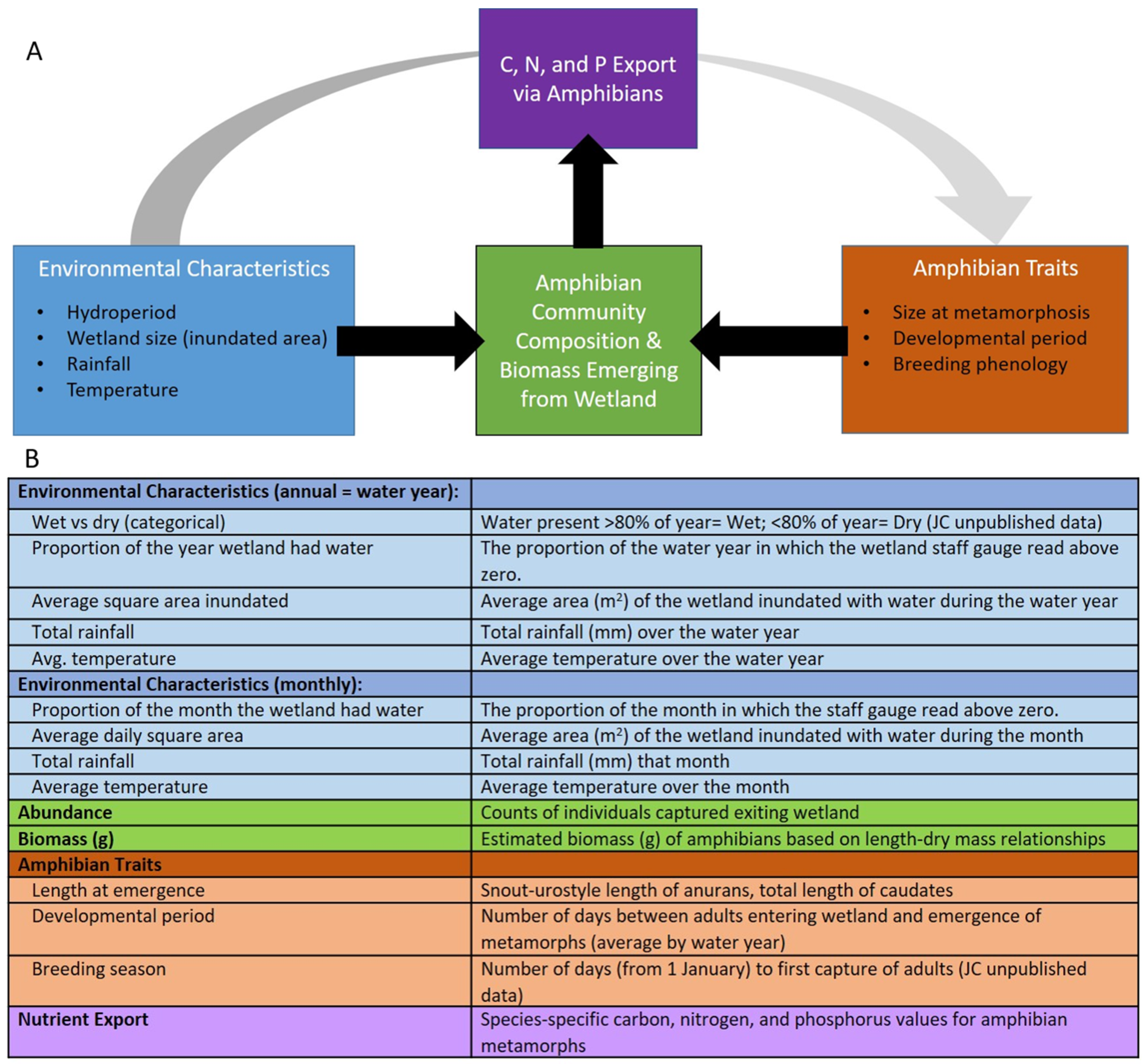
Most studies to date that have quantified amphibian export, have focused on a single season [14,26] or species-poor communities with low variation in associated life-history traits [22]. Our goal was to quantify amphibian diversity, abundance and biomass export in two isolated wetlands using a long-term study in the biodiverse southeast USA. We then combine our count and biomass data with data on tissue stoichiometry (C, N and P) of late-stage larva of 11 species of salamanders and frogs (i.e., urodeles and anurans) collected in another study [30] to generate estimates of the annual export for nutrients by amphibians from the two wetlands. We also wanted to identify factors that influence the timing and magnitude of amphibians exported from isolated wetlands as a first step to quantifying the movements of amphibians and the nutrients they transport from wetlands to surrounding upland landscapes. Therefore, we couple environmental data with count data of juveniles to explore the controls of amphibian diversity, production and export and the amphibian life-history traits that are associated with export over varying environmental conditions (Figure 1A).
2. Materials and Methods
2.1. Study Site
We conducted this study at the Jones Center at Ichauway (hereafter Ichauway) located in the lower Gulf Coastal Plain (elevation = ~50 m above sea level) in Baker County, Georgia, USA. Ichauway is an 11,700-ha research site with mature longleaf pine (Pinus palustris) forest and more than 100 isolated depressional wetlands. Our study focused on quantifying the diversity and magnitude of amphibians exiting two small wetlands and identifying the environmental factors related to the diversity, abundance and biomass of the amphibians. The first wetland, W41, is a forested depression that is 1500 m2 in size with large live oak (Quercus virginiana), water oak (Q. nigra) and slash pine (Pinus elliottii) in the overstory, and little emergent vegetation. The second wetland, W51, is 7300 m2 in size and is a marsh, dominated by maidencane (Panicum hemitomon) and Juncus repens with buttonbush (Cephalanthus occidentalis) and a few blackgum tupelo (Nyssa sylvatica) in the deepest portion of the wetland. Wetland 51 was initially surrounded by large live oak, laurel oak (Q. laurifolia) and water oak, which were mechanically removed late in 2009 as part of a separate study on the effects of hardwood removal on wetland hydrology [31].
2.2. Temperature, Rainfall and Wetland Hydrology
The Jones Center maintains a long-term meteorological station from which we obtained the average, minimum and maximum air temperature and daily rainfall totals for the study area (Georgia Automated Environmental Monitoring Network). Staff gauges were deployed on 25 May 2005 at W41 and on 20 June 2005 at W51 in the deepest portion of each wetland and monitored for depth approximately biweekly to the nearest 0.01 m. Based on elevation data collected at 0.25 m intervals within the wetland, we estimated the percent of the total area of the wetland that was inundated at each staff gauge reading. Since staff gauge data were not available for the beginning of the amphibian sampling for W51, we modeled the predicted percent inundation of that wetland by using data from another wetland (W02) where data were available dating back to 2003 (Jones Center, unpublished data). We examined the correlation between W02 and W51 during the time period in which both wetlands had data available from the same day (5 July 2005 through 28 December 2011). We used linear regression to correlate the percentage of the basin that was full for the two wetlands to derive an equation to predict the water level of W51 going back to 1 January 2002.
To calculate hydroperiod length per water year (1 October to 30 September), we subtracted the number of days between dry staff gauge measurements from 365 days. If the wetland did not dry within a full water year, its hydroperiod length was recorded as 365 days. Only consecutive staff gauge measurements lasting over 30 days indicating inundation counted towards yearly hydroperiod length. If a dry period extended between water years, we subtracted the start of the dry period to 30 September for the first water year, and subtracted from 1 October to the end of the dry period for the second water year. We then calculated the proportion of the water year in which wetlands contained water. We also calculated the proportion of the water year in which the wetland was completely full (at maximum staff gauge height and covering the entire surface area). We categorized the year as wet (versus dry) if W51 had water more than 80% of the water year (Figure 1B) and was full (completely inundated) more than 50% of the time (Table 1). This categorization helped control for antecedent conditions in water level and hydroperiod from the year before.
2.3. Amphibian Sampling Methods
We used terrestrial drift fences encircling the wetlands to quantify the amphibian movements [32,33]. Fences consisted of a 0.60 m tall aluminum flashing that was buried ca. 15 cm below ground. The drift fence at W41 had paired pitfall traps at 20 m intervals that were installed in November 2005 and the traps were monitored through June 2008, when the wetland was inundated (Table 1). At W51, 22 pairs of screen funnel traps [32] were placed at 20-m intervals around the fence to capture amphibians from October 2002 through April 2004. In May 2004, funnel traps were replaced with 22 pairs of pit fall traps (19-l buckets) installed at the original trap stations and traps were monitored through 2011. Both funnel and pit fall traps contained sponges that were wetted regularly to prevent amphibians from desiccating. When the wetlands were dry, the traps were temporarily closed and gaps were opened in the fence to allow free movement of amphibians. Traps at both wetlands were checked six days a week and all amphibians captured were identified to species; snout-vent length was measured for salamanders, snout-urostyle length was measured for frogs and all individuals were assigned a sex/life stage (adult female, adult male, juvenile and metamorph [34,35]). In some cases, individuals were weighed, or during synchronous emigration events, 30 individuals were weighed to determine an average mass and metamorphs were subsequently weighed en masse and abundance data were estimated from these totals. After measurements were taken, amphibians were released on the opposite side of the fence from their point of capture.
2.4. Biomass, Nutrient Flux and Species Traits
We estimated the amount of dry mass (g) of emerging metamorphic amphibians exported from each of the wetlands each month and across the annual hydroperiod using wet mass to dry mass relationships (Knapp, unpublished data; Supplement Table S1). However, since the wet masses from Knapp (unpublished data) were measured post-intestinal removal, we conservatively estimated that the intestinal tract of the larvae was 5% of the overall body mass (see [36]). Therefore, we subtracted 5% of the wet mass from each individual caught within the drift fences before converting to dry mass. For amphibian body nutrient content data, we used data from another study conducted at Ichauway [30] on the carbon (C), nitrogen (N) and phosphorus (P) content of 11 species just before emergence. As the body stoichiometry of one species caught within this study, Anaxyrus terrestris, was unmeasured from Knapp et al. (2021) [30], we used the stoichiometric measurements from Luhring et al. (2017) [37] for this species. These data were used to estimate the water year nutrient export by amphibians exiting our two study wetlands. We calculated the C, N and P export by amphibians by taking the product of our species-specific dry mass estimates and species- or genus-specific C, N and P nutrient content of amphibians from Knapp et al. (2021) [30] and Knapp (unpublished data). This was then summed across the water year to estimate the total annual nutrient export (nutrient y−1) by amphibians. See Knapp et al. (2021) [30] for interspecific differences in nutrient content, but generally tissue stoichiometry was similar within genera.
3. Data Analyses
We examined variation in amphibian species richness across years using total species richness and Shannon diversity across years within both wetlands using the vegan package in R. Then, to investigate the drivers of amphibian flux from wetlands and the associated nutrient export, we examined the environmental factors that contribute to community export. To do this we used the longer-term dataset from W51 and conducted a non-metric multidimensional scaling (NMDS) at two different temporal scales to examine how the community assemblage in W51 varied. First, we used NMDS to examine the annual patterns (among years) in juvenile amphibian count data within a year at W51. To test for differences in amphibian community composition between “wet” and “dry” years, we used a permutational multivariate analysis of variance (PERMANOVA; [38]) to determine if the proportion of the year that the wetland was full (high year when the wetland was full contained water >80% of the year) was an important driver of amphibian community composition. We also explored relationships among annual amphibian community composition, average annual wetland square area, total annual rainfall, average annual temperature, and the proportion of the year the wetland held water (Figure 1B) by fitting these environmental vectors onto the NMDS ordination space using the vegan function ‘envfit’. Then, we used our more fine-scaled temporal data of monthly juvenile amphibian count data across all years at W51 to examine patterns in community composition across all months and years using NMDS, excluding the months where no amphibians were captured. Relationships among amphibian community composition, the proportion of the month that the wetland held water, the average daily square area of the wetland, monthly total rain, and average daily temperature over the month (Figure 1B; Supplements, Table S2) were examined by fitting these environmental vectors onto the NMDS ordination space using the vegan function ‘envfit’. The significance of the fitted vectors was assessed using a permutation procedure (1000 permutations) (Oksanen et al., 2008). We followed this with a manyGLM in the mvabund package to determine the relationship between specific significant factors and community members using our full monthly data series.
To further test predictors of interspecific variation in the environmental conditions affecting amphibian emergence, we compiled a set of three life-history traits for each of our species collated from our own data and published sources (Table S3): average length at emergence (mm), average development period (days), and breeding season, which was the day an individual of a given species was first collected (number of days from January 1st). Then, to investigate which amphibian traits were associated with the environmental variables and abundance at emergence, we used the model-based approach fourth corner analysis [39]. Fourth-corner analysis examines the environment–trait associations and conceptualizes them as a set of four matrices: abundances of species, trait data by species, environmental data by date and environmental data by traits, with the relationships of this last corner being estimated [40]. The resulting environment–trait interaction coefficients show how the environmental response across taxa varies as traits vary. The size of the coefficients is a measure of importance, and coefficients are interpreted as the amount by which a unit (1 SD) change in the trait variable changes the slope of the relationship between abundance and a given environmental variable. To estimate these coefficients, we used a negative binomial regression (package ‘mvabund’, [41]).
4. Results
4.1. Environmental Conditions
Over our nine years of study there was low variation in the annual average temperature, but variation in rainfall resulted in high variation in wetland hydrology (Table 1). In particular, 2006–2008 and 2011 were “dry” years in which the proportion of the year that W51 was inundated was <80%, the wetland was full <32% of the water year and the average area of the wetland filled never exceeded 2200 m2 (30% full), while wet years were characterized by the average area of the wetland filled exceeding 5000 m2 (68% full). The percent of the total area of each wetland that was inundated each year varied dramatically, but both wetlands were relatively dry from the end of 2006 through early 2008 and 2011 was dry (Supplements, Table S2, Figure S1).
4.2. Amphibian Diversity and Abundance
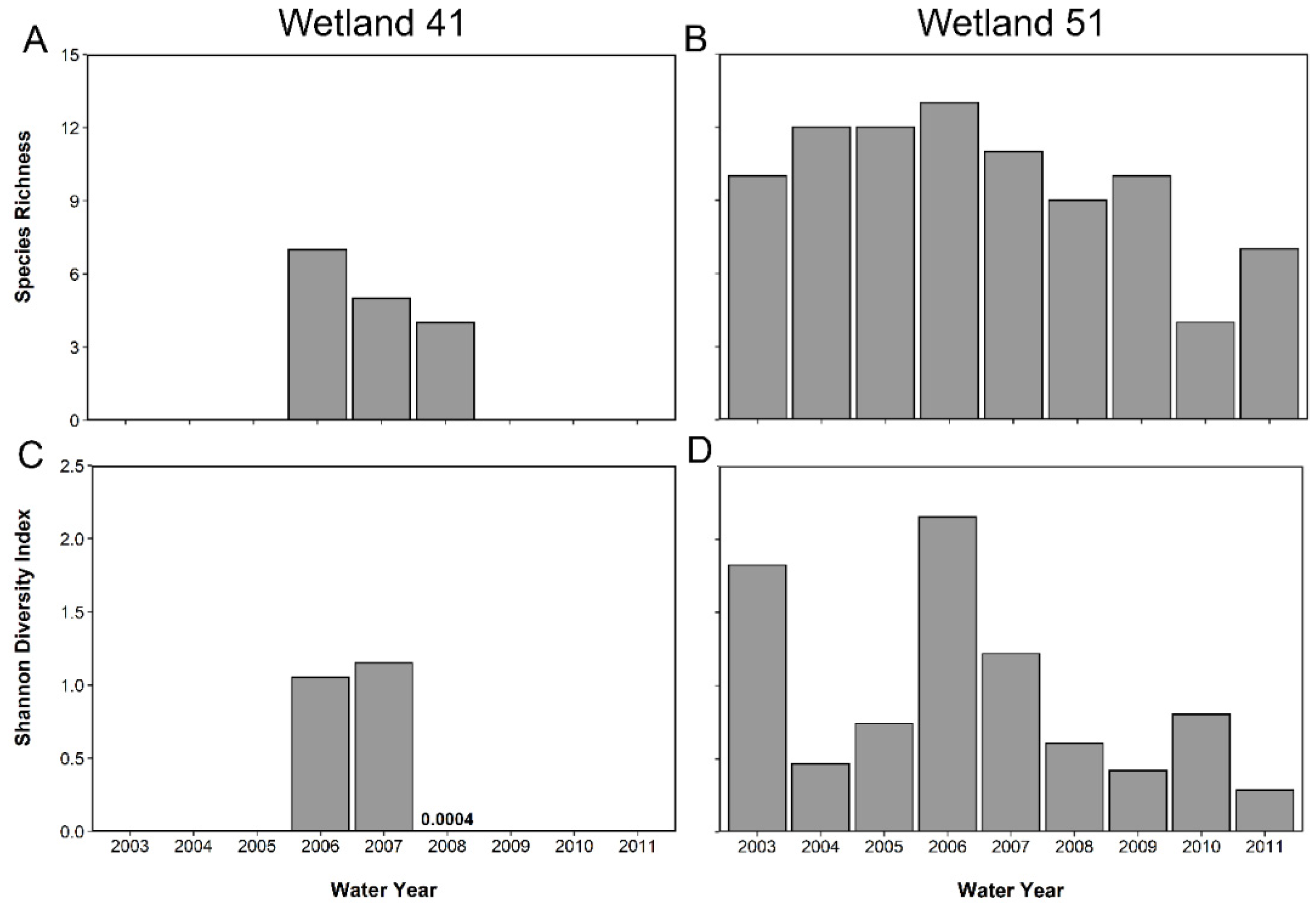
We captured 13 amphibian species in total across all years of the study (Table 2 and Table S4). We captured ten species over three years of study in W41 (Figure 2A) and 13 species over nine years at W51 (Figure 2B). Total diversity in a given year ranged from 4 to 7 in W41 and 4 to 13 in W51, highlighting the high degree of variation between the wetlands and among years (Figure 2A,B). Shannon diversity ranged from 0.0004 in 2008 to 1.15 in 2007 at W41 (Figure 2C). In W51, Shannon diversity ranged from 0.42 in 2009 to 2.15 in 2006 (Figure 2D). W41 was dominated by Scaphiopus holbrookii in 2008 in terms of abundance and biomass due to a large emergence of that species (N = 310,443), while in other years W41 produced far fewer juveniles and was dominated numerically by Gastrophryne carolinensis (N = 249, Table 2; Figure 3A). W51, with a more diverse community and a longer-term record, was dominated numerically by A. terrestris (N = 37,824), G. carolinensis (N = 13,146) and Pseudacris ornata (N = 9034) (Table 2; Figure 3B). The areal annual flux of amphibians also varied dramatically across years in among the two study wetlands with areal emergence being as low as 0.01 ind m−2 y-1 in W51 in 2010 to as high 310 ind m−2 y−1 in W41 in 2008 (Table 3).
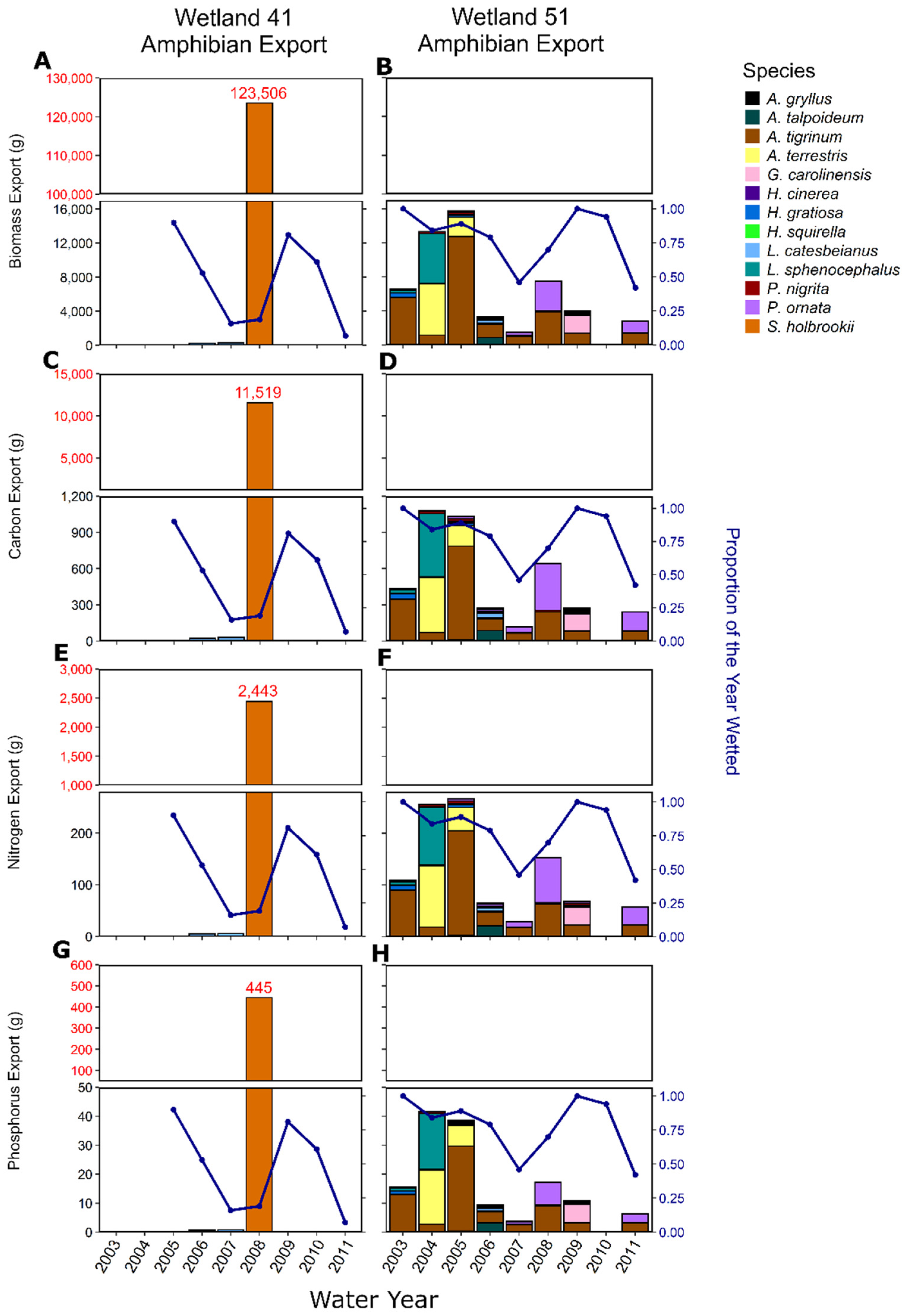
Biomass flux by juvenile amphibians varied dramatically across years and across wetlands (Supplementary Table S5). Average total flux of amphibian biomass 2006–2008 in W41 was 8742 ± 15,040 g DM y−1 (mean ± standard deviation) and ranged from 52 to 26,108 g DM y−1, with the high flux in 2008 being associated with a large number of Scaphiopus holbrookii (Figure 3A). Other than 2008, W41 tended to have a lower flux of amphibian biomass than W51 and was dominated by L. catesbeianus (96.5 g total) and G. carolinensis (6.7 g) (Table 2). The average flux of amphibian biomass (2003–2011) in W51 was 1021 ± 895 g DM y−1 and ranged from 4.3 g DM y−1 in 2010 to 2556 g DM y−1 in 2005 (Figure 3B). W51 amphibian biomass export was dominated by Ambystoma tigrinum (3806 g total), P. ornata (1331 g) and L. sphenocephalus (1266 g) (Table 2). Areal annual biomass flux of amphibians varied dramatically across years with the average annual areal biomass emergence being 0.14 ± 0.12 g m−2 y−1 in W51 and 8.74 ± 15.04 g m−2 y−1 in W41, when considering all years, and 0.06 ± 0.01 g m−2 y−1 in W41 when excluding 2008, the year with the large Scaphiopus holbrookii emergence (Table 3).
Biomass was the dominant control of consequential nutrient fluxes from the wetlands into the uplands by amphibian juveniles, but species composition also played an important role. Carbon, N and P fluxes varied dramatically as a result of both of these factors (Figure 3C–H). Across the two wetlands, total annual C flux ranged from 25 to 11,519 g C y−1 in W41 (Figure 3C) and 1.9 to 1077.7 g C y−1 in W51 (Figure 3D). Total N fluxes ranged from 5.1 to 2442.8 g N y−1 in W41 (Figure 3E) and 0.4 to 266 g N y−1 in W51 (Figure 3F). Total P fluxes were similarly variable, ranging from 0.7 to 445.4 g P y−1 in W41 (Figure 3G) and 0.06 to 38.7 g P y−1 in W51 (Figure 3H). Areal-corrected nutrient fluxes also varied dramatically across years and the two wetlands (Table 3). For the years in which the study overlapped in the two wetlands (2006–2008), amphibians exported ~7x more C, N and P from W51 in 2006 and 2007 (mean; C = 196.2 mg C m−2 y−1, N = 47.4 mg N m−2 y−1, P = 6.6 mg P m−2 y−1) than W41 (mean; C = 28.4 mg C m−2 y−1, N = 5.6 mg N m−2 y−1, P = 0.8 mg P m−2 y−1). However, in 2008, primarily as a result of S. holbrookii, amphibians exported ~18x more C, N and P from W41 than was exported from W51 (Table 3).
4.3. Environmental Drivers of Amphibian Community Composition at W51
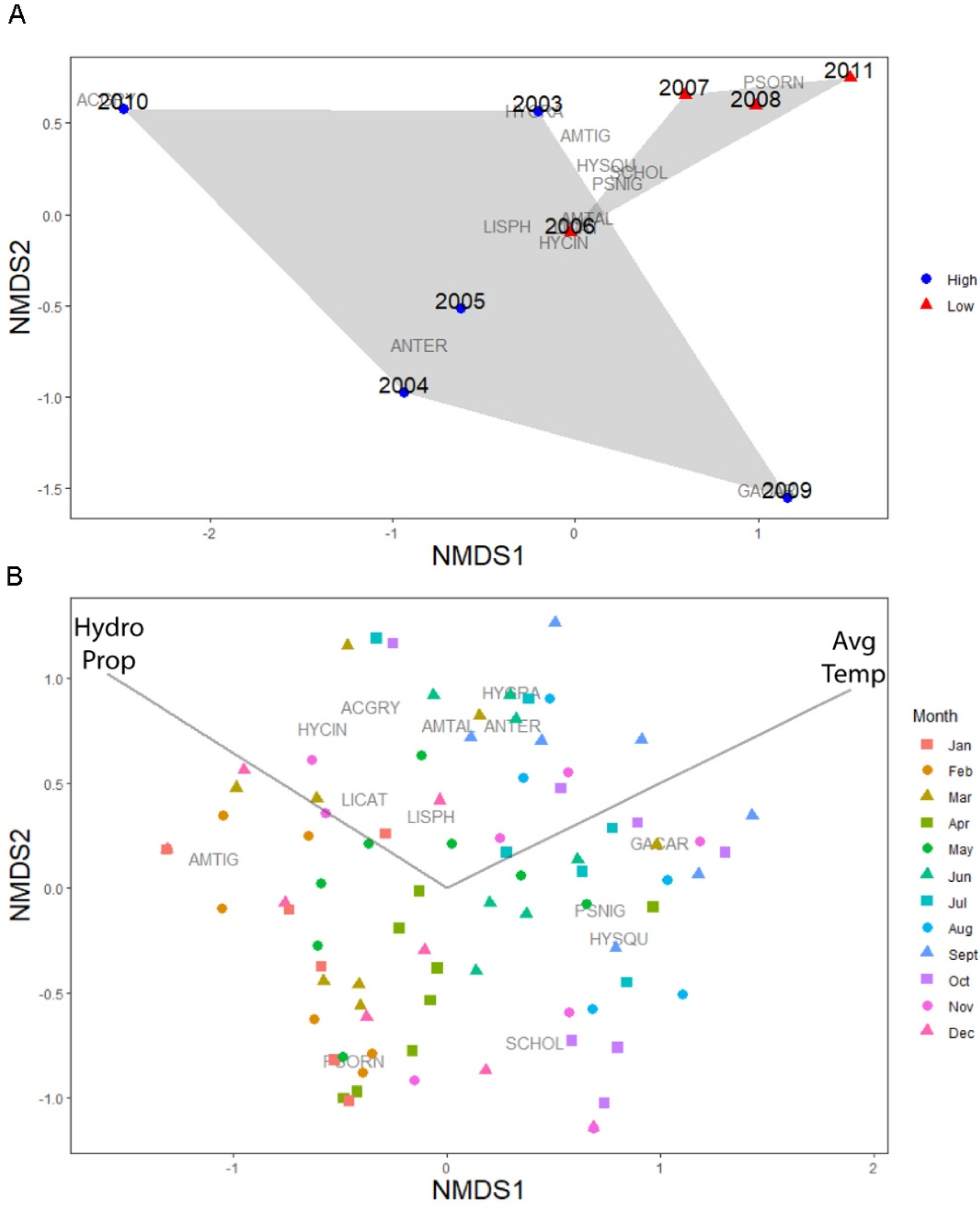
The amphibian community composition varied across years, as shown by the NMDS (non-metric fit R2 = 0.99, Stress < 0.06; Figure 4A). There were not any significant predictors of annual amphibian community export (all predictors p > 0.10). However, the PERMANOVA indicated that the proportion of time the wetland held water (i.e., hydroperiod) impacted the resulting community composition of the metamorphs exiting the wetland (PERMANOVA, pseudo-F1,8 = 2.96, R2 = 0.30, p = 0.02). In particular, years in which the wetland had longer hydroperiods there was higher relative abundances of metamorph L. sphenocephalus, Anaxyrus terrestris and Ambystoma tigrinum, three of the dominant species captured in W51.
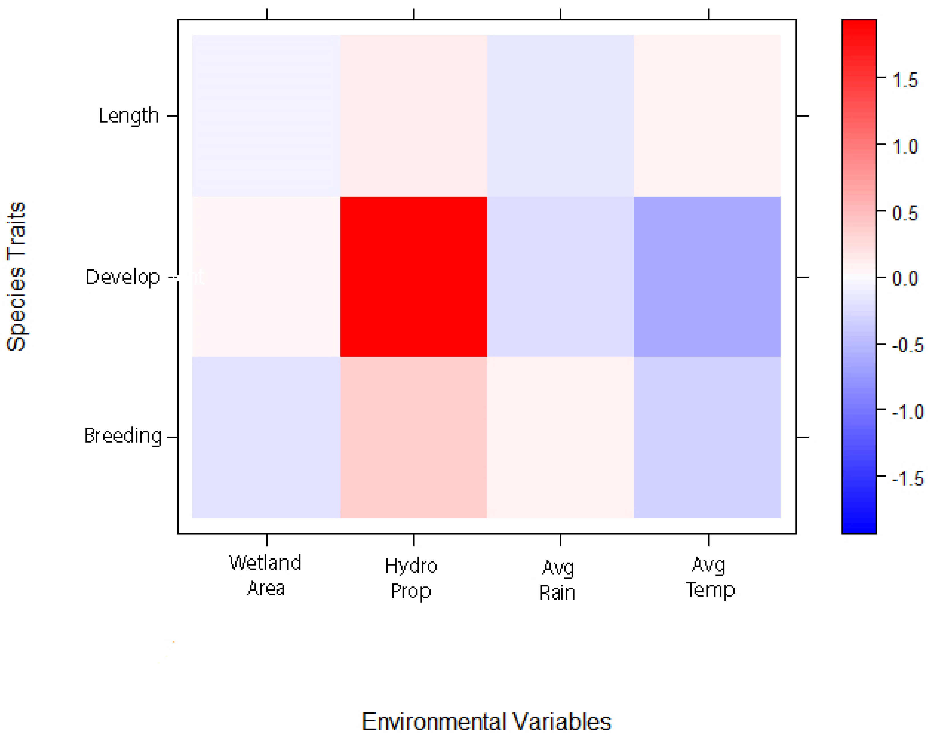
When examining the monthly data, our NMDS indicated that community composition varied (non-metric fit = 0.95, Stress < 0.04; Figure 4B) and generally clustered by month. Joint plot analysis indicated that the average daily temperature (F = 8.13, R2 = 0.050, p < 0.001), the proportion of the month that the wetland held water (F = 5.89, R2 = 0.26, p < 0.001) and the interaction between these two variables (F = 3.13, R2 = 0.03, p < 0.001) influenced the relative abundance of community export. When examining the full dataset using manyGLM, the monthly amphibian community exiting W51 was influenced by the proportion of the time the wetland held water (Dev1,106 = 86.72, p = 0.002) and the average daily temperature (Dev1,105 = 120.14, p = 0.001), but not the interaction between the two (Dev1,104 = 20.24, p = 0.14). In particular, Anaxyrus terrestris, Pseudacris nigrita (multiGLM, p < 0.01) and L. sphenocephalus (p = 0.09) export was associated with warmer temperatures and Hyla squirella was impacted by the interaction between the proportion of time W51 was wetted and temperature (p = 0.02). Further examination of our monthly time series data revealed that species traits were marginally related (p = 0.09) to the measured environmental factors (Figure 5). In particular, species developmental period, breeding season and body length at emergence were positively related to the proportion of the time the wetland held water while development and breeding season were negatively related to average daily temperature.
5. Discussion
We documented high temporal variability of amphibian export and community composition in small, isolated wetlands that could partly be explained by hydroperiod and life-history traits. Generally, wetter years resulted in higher amphibian biomass export and resultant nutrient export, but this was highly variable due to the diversity of life-history traits in this species-rich community. We also saw large differences in species composition and juvenile production between the two study wetlands in the overlapping years of study, suggesting both high spatial and temporal variability in amphibian export. Differences in wetland vegetation type and landscape position, in addition to environmental variables, may explain spatial variability in export [42,43].
5.1. Amphibian Species Diversity and Biomass Export
We found that these two small wetlands collectively supported a diverse amphibian community, and, in wetter years, they tended to produce a high abundance and biomass of emerging juveniles. Gibbons et al. (2006) [26] were among the first to note the extremely high diversity (14 species), abundance and biomass of emerging amphibians from a single year of study in a much larger (10 ha) wetland in South Carolina. While the wetland studied by Gibbons et al. (2006) [26] was larger, diversity was similar in these smaller wetlands, and when scaled for area, both W41 and W51 sometimes exceeded the abundances (Table 3) found in that study (3.6 ind. m−2). Fritz et al. (2021) [15] found that while larger wetlands produced greater total fluxes of amphibians to uplands, smaller wetlands were typically more productive per unit area. Thus, they suggested that a mosaic of small ponds may result in greater or equal fluxes of amphibians to upland food webs than a single large pond. Given the ubiquity of wetlands in our study region [44], our study underscores the important role amphibians have in linking wetland habitats to surrounding uplands.
5.2. Amphibian Nutrient Export
Larval amphibians have been shown to strongly regulate nutrient cycling and primary production in wetlands, with their metamorphosis and emergence typically resulting in a net export of nutrients [19,21,22]. Nutrient fluxes from our two study wetlands varied mostly due to the total biomass of the emerging community, but also partially due to species-specific stoichiometry. The abundance (this study) and tissue stoichiometry [30] of amphibians varied as a result of functional traits. Knapp et al. (2021) [30] found that stoichiometry varied due to life-history traits, where body size and time to development were positively related to %C and C:N and were negatively related to %P if the Lithobates spp. were removed. This suggests that not only will specific life-history traits of the associated amphibian communities change in response to environmental factors, but also the nutrient fluxes associated with these communities.
Although amphibians perform an important ecological role in transferring energy between trophic levels in some forest ecosystems [45,46], their role as links between aquatic and terrestrial food webs is only beginning to be studied, especially in species-rich systems. These wetlands are often N or P limited [8,47] and the export of nutrients by amphibian communities may represent an important wetland nutrient sink in some years [22,48]. While our study only considered the movement of amphibians, leaving the wetlands and moving into the terrestrial system, our study encompassed a wide variety of environmental conditions. In a single wetland, the species that emerged varied across years with wetter years typically resulting in higher emergence and nutrient export. Similarly, Balik et al. [49] showed that more permanent ponds in the mountain west had higher invertebrate and salamander biomass, which resulted in communities within permanent ponds to provide more in-pond nutrients via their excretion than communities in temporary ponds. In comparison with previous studies, exports of amphibian nutrients from our study wetlands were similar to exports of wood frogs (Lithobates sylvaticus; mean = 0.35 g C m−2 y−1; 0.09 g N m−2 y−1; and 0.02 g P m−2 y−1) from a pond in Michigan [22], but our estimates were much more variable across years given our multi-species communities. We were unable to quantify nutrient import into these wetlands via the deposition of egg masses, but most studies have generally found a net nutrient export by emerging amphibians [15,22]. Similar to emerging aquatic insects, metamorphosed amphibians are a high-quality food source for predators in adjacent habitats [46,50,51]. Thus, our study highlights the mass flux of nutrients resulting from these small wetlands via amphibians.
5.3. Hydroperiod and Temperature as Environmental Controls on Amphibian Emergence
While we observed some differences in community composition and overall flux in response to wetland hydroperiod and temperature, our predictor variables were weak in explaining amphibian community emergence. Previous work has indicated that local species richness is sensitive to water availability during the breeding season, but in the southeast, longer hydroperiods had a negative effect on amphibian persistence [52]. Overall, species richness has been shown to be driven by hydroperiod with weak relationships showing higher richness with longer hydroperiods, but also patterns in species turnover with hydroperiod [6]. Our species trait analysis gave us better insight into what amphibian traits are favored under various environmental conditions. For example, the number of days to development is extended and larger bodied taxa emerge when there is a longer hydroperiod while higher temperatures promote amphibians with earlier breeding seasons and shorter development times. In W51, where we had a longer-term dataset, the abundance of emerging juveniles decreased during dry years (2006–2008) and the community composition shifted from a dominance of slower-developing species (L. sphenocephalus and A. tigrinum) to faster-developing species (P. ornata and G. carolinensis) (Figure 4). During later wet years (2009 and 2010), previously dominant species were much less abundant, suggesting that antecedent conditions might have long-term effects on the amphibian community. However, the hardwood removal treatment in the W51 catchment area that occurred in 2009 [31] may also have affected the amphibian community and confounded our results. This may explain the low abundance of A. terrestris following the hardwood removal as this species has a short development period, but often inhabits hardwood hammocks [32]. Interestingly, W41, which experienced infrequent short periods of inundation (JC, unpublished data), produced the greatest amphibian biomass and nutrient export in our study. Wetland 41 also produced a few metamorph L. catesbeianus, which is a species with a particularly long development period (Knapp 2021), thus showing that even short hydroperiod wetlands can be highly productive in some years and support species with a variety of life-history traits.
Given the high degree of variance and the complex interactions among biotic and abiotic factors and the high species diversity of this community, it is difficult to disentangle the specific drivers of amphibian community composition and biomass. For example, years with greater water permanence may reduce larval survival due to predation while short hydroperiods can result in drying, leading to mortality [53,54,55]. Thus, there are multiple compounding factors and factors that we did not measure here controlling amphibian export. Fritz et al. (2021) [15] similarly found that hydroperiod was an important driver of amphibian emergence, but terrestrial insect input was also an important predictor of total amphibian emergence. Terrestrial insect inputs to isolated wetlands have not been studied in relation to other inputs, but Fritz et al. (2021) [15] suggest that the insect inputs are a high-quality subsidy enhancing amphibian production, especially salamander larvae. This suggests that factors other than hydroperiod, including the surrounding terrestrial inputs, are drivers controlling amphibian export, which need to be explored in the future.
5.4. Future Changes in Land Use and Climate—Consequences for Amphibian Diversity and Export
Due to their small size and often short hydroperiods, isolated wetlands are regularly overlooked and, without regulatory protections, are often modified for agricultural and urban use, leading to large-scale alterations to wetlands or direct losses in wetland habitat [56]. Our study region of southwestern Georgia has experienced an increase in irrigated agriculture [57]. This has resulted in the loss of some wetlands but many wetlands remain on the landscape with highly altered vegetation and sometimes receiving irrigation water thus extending the hydroperiod [58]. In addition, wetlands in the agricultural landscape often have higher nutrient and bacterial concentrations [59], with the impacts to amphibian diversity and export being unknown. Moreover, wetlands in southeastern pine forests may be impacted by hardwood encroachment resulting from fire suppression [5]. Golladay et al. (2021) [31] found that removal of hardwoods around W51 increased the hydroperiod by 50 days in wet years and 53 days in dry years. Amphibian diversity, productivity, and nutrient flux in altered wetlands and within agricultural lands warrants further study.
Alterations in precipitation and temperature due to climate change could shorten or alter the timing of wetland hydroperiods, threatening the communities that depend on them [31,60,61]. Climate change is known to have a host of direct and indirect impacts on amphibian communities, including effects on survival, growth, reproduction and dispersal capabilities, as well as shifting habitat suitability and affecting disease transmission [62]. Here we noted that both the proportion of the year in which the wetlands contained water and the temperature were factors in amphibian community assembly, which suggests how changes in the timing and magnitude of precipitation could alter amphibian export.
6. Conclusions
Continued amphibian population declines and extinctions will likely have large-scale and long-lasting effects on ecosystems [63,64]. Quantifying changes in amphibian species diversity and richness is essential for understanding changes in the structure of affected ecosystems [65,66]. Our findings underscore the key role of small, isolated wetlands and their hydroperiod characteristics in maintaining amphibian productivity and community dynamics by coupling aquatic habitats with adjacent terrestrial habitats via transfer of biomass and nutrients. Patterns of land-use and climate change are threatening seasonal wetlands around the world; thus, it is likely that individual wetlands and the linkages between them and other aquatic habitats will continue to decline or be lost entirely. Given the multitude of threats to wetlands, and their connections to surrounding upland forests, future studies should take a holistic approach to further understanding the links among wetlands, upland forests and the role of isolated wetlands at a landscape scale.
Supplementary Materials
The following are available online at https://0-www-mdpi-com.brum.beds.ac.uk/article/10.3390/d13110598/s1 Table S1: Average mass of individuals captured, proportion of wet mass to dry mass, and proportion of carbon, nitrogen, and phosphorus for each species, Table S2: Monthly environmental data from W51 and the on-site weather station used in the NMDS and manyGLM analyses, Table S3: Life history traits of our focal species used in the fourth-corner analysis, Table S4: Species richness and Shannon diversity across each sampling year, Table S5: Total counts, biomass (dry mass; DM), C, N, and P exported by amphibians by year in W41 and W51, Figure S1: Percent of the total area of W41 and W51 that were inundated during the study.
Author Contributions
Conceptualization, C.L.A. and L.L.S.; methodology, C.L.A., L.L.S. and D.D.K.; formal analysis, C.L.A. and D.D.K.; writing—original draft preparation, C.L.A.; writing—review and editing, C.L.A., L.L.S. and D.D.K.; visualization, C.L.A. and D.D.K.; funding acquisition, L.L.S. All authors have read and agreed to the published version of the manuscript.
Funding
This research was funded by the Robert W Woodruff Foundation.
Institutional Review Board Statement
We followed the Herpetological Animal Care and Use Committee Guidelines of the American Society of Ichthyologists and Herpetologists (http://www.asih.org/files/hacc-final.pdf (accessed on 15 September 2021)).
Data Availability Statement
Data is reported in tables throughout the article and in the supplementary materials and held at the Jones Center at Ichauway.
Acknowledgments
We thank C. Borg, D. Steen, J. Howze and numerous research technicians for installing drift fences and recording field data for this project. B. Clayton surveyed the study wetlands and collected staff bi-weekly gauge data. J. Brock edited the wetland survey data to create contour maps. This research was conducted under Georgia Department of Natural Resources permit Nos. 29-WMB-02-86, 29-WMB-03-142, 29-WMB-04-188, 29-WTN-05-166, 29-WTN-06-109, 29-WBH-08-161, 29-WBH-09-151, 29-WBH-10-109.
Conflicts of Interest
The authors do not declare a conflict of interest.
References
- Leibowitz, S.G. Isolated wetlands and their functions: An ecological perspective. Wetlands 2003, 23, 517–531. [Google Scholar] [CrossRef]
- Kirkman, L.K.; Smith, L.L.; Quintana-Ascencio, P.F.; Kaeser, M.J.; Golladay, S.W.; Farmer, A.L. Is species richness congruent among taxa? Surrogacy, complementarity, and environmental correlates among three disparate taxa in geographically isolated wetlands. Ecol. Indic. 2012, 18, 131–139. [Google Scholar] [CrossRef]
- EPA. Connectivity of Streams and Wetlands to Downstream Waters: A Review and Synthesis of the Scientific Evidence; EPA/600/R-14/475F; US Environmental Protection Agency: Washington, DC, USA, 2015.
- Cohen, M.J.; Creed, I.F.; Alexander, L.; Basu, N.B.; Calhoun, A.J.; Craft, C.; D’Amico, E.; DeKeyser, E.; Fowler, L.; Golden, H.E. Do geographically isolated wetlands influence landscape functions? Proc. Natl. Acad. Sci. USA 2016, 113, 1978–1986. [Google Scholar] [CrossRef] [Green Version]
- Smith, L.L.; Subalusky, A.L.; Atkinson, C.L.; Kirkman, L.K. Ecology and Restoration of the Longleaf Pine Ecosystem. In Geographically Isolated Wetlands: Embedded Habitats in Longleaf Pine Forests; Kirkman, L.K., Jack, S.B., Eds.; CRC Press: Boca Raton, FL, USA, 2017. [Google Scholar]
- Snodgrass, J.W.; Komoroski, M.J.; Bryan, A.L.; Burger, J. Relationships among isolated wetland size, hydroperiod, and amphibian species richness: Implications for wetland regulations. Conserv. Biol. 2000, 14, 414–419. [Google Scholar] [CrossRef]
- Griffiths, R.A. Temporary ponds as amphibian habitats. Aquat. Conserv. Mar. Freshw. Ecosyst. 1997, 7, 119–126. [Google Scholar] [CrossRef]
- Battle, J.; Golladay, S.W. Water quality and macroinvertebrate assemblages in three types of seasonally inundated limesink wetlands in southwest Georgia. J. Freshw. Ecol. 2001, 16, 189–207. [Google Scholar] [CrossRef] [Green Version]
- Leeper, D.A.; Taylor, B.E. Abundance, biomass and production of aquatic invertebrates in Rainbow Bay, a temporary wetland in South Carolina, USA. Archiv Hydrobiol. 1998, 143, 335–362. [Google Scholar] [CrossRef]
- Stubbington, R.; Datry, T. The macroinvertebrate seedbank promotes community persistence in temporary rivers across climate zones. Freshw. Biol. 2013, 58, 1202–1220. [Google Scholar] [CrossRef] [Green Version]
- Subalusky, A.L.; Fitzgerald, L.A.; Smith, L.L. Ontogenetic niche shifts in the American Alligator establish functional connectivity between aquatic systems. Biol. Conserv. 2009, 142, 1507–1514. [Google Scholar] [CrossRef]
- Williams, D.D.; Hynes, H.N. The ecology of temporary streams I. The faunas of two Canadian streams. Int. Rev. Der Gesamten Hydrobiol. Hydrogr. 1976, 61, 761–787. [Google Scholar] [CrossRef] [Green Version]
- Schofield, K.A.; Alexander, L.C.; Ridley, C.E.; Vanderhoof, M.K.; Fritz, K.M.; Autrey, B.C.; DeMeester, J.E.; Kepner, W.G.; Lane, C.R.; Leibowitz, S.G.; et al. Biota Connect Aquatic Habitats Throughout Freshwater Ecosystem Mosaics. JAWRA J. Am. Water Resour. Assoc. 2018, 54, 372–399. [Google Scholar] [CrossRef]
- Fritz, K.A.; Whiles, M.R. Amphibian-mediated nutrient fluxes across aquatic–terrestrial boundaries of temporary wetlands. Freshw. Biol. 2018, 63, 1250–1259. [Google Scholar] [CrossRef]
- Fritz, K.A.; Whiles, M.R. Reciprocal subsidies between temporary ponds and riparian forests. Limnol. Oceanogr. 2021, 66, 3149–3161. [Google Scholar] [CrossRef]
- Hannan, L.B.; Roth, J.D.; Ehrhart, L.M.; Weishampel, J.F. Dune vegetation fertilization by nesting sea turtles. Ecology 2007, 88, 1053–1058. [Google Scholar] [CrossRef]
- Holtgrieve, G.W.; Schindler, D.E. Marine-derived nutrients, bioturbation, and ecosystem metabolism: Reconsidering the role of salmon in streams. Ecology 2011, 92, 373–385. [Google Scholar] [CrossRef]
- Booth, M.T.; Hairston Jr, N.G.; Flecker, A.S. Consumer movement dynamics as hidden drivers of stream habitat structure: Suckers as ecosystem engineers on the night shift. Oikos 2020, 129, 194–208. [Google Scholar] [CrossRef]
- Seale, D.B. Influence of amphibian larvae on primary production, nutrient flux, and competition in a pond ecosystem. Ecology 1980, 61, 1531–1550. [Google Scholar] [CrossRef]
- Moore, J.W.; Schindler, D.E.; Carter, J.L.; Fox, J.; Griffiths, J.; Holtgrieve, G.W. Biotic control of stream fluxes: Spawning salmon drive nutrient and matter export. Ecology 2007, 88, 1278–1291. [Google Scholar] [CrossRef] [PubMed] [Green Version]
- Regester, K.J.; Lips, K.R.; Whiles, M.R. Energy flow and subsidies associated with the complex life cycle of ambystomatid salamanders in ponds and adjacent forest in southern Illinois. Oecologia 2006, 147, 303–314. [Google Scholar] [CrossRef] [PubMed]
- Capps, K.A.; Berven, K.A.; Tiegs, S.D. Modelling nutrient transport and transformation by pool-breeding amphibians in forested landscapes using a 21-year dataset. Freshw. Biol. 2015, 60, 500–511. [Google Scholar] [CrossRef]
- Sitters, J.; Atkinson, C.L.; Guelzow, N.; Kelly, P.; Sullivan, L.L. Spatial stoichiometry: Cross-ecosystem material flows and their impact on recipient ecosystems and organisms. Oikos 2015, 124, 920–930. [Google Scholar] [CrossRef]
- Polis, G.A.; Anderson, W.B.; Holt, R.D. Toward an integration of landscape and food web ecology: The dynamics of spatially subsidized food webs. Annu. Rev. Ecol. Syst. 1997, 28, 289–316. [Google Scholar] [CrossRef] [Green Version]
- Leroux, S.J.; Loreau, M. Subsidy hypothesis and strength of trophic cascades across ecosystems. Ecol. Lett. 2008, 11, 1147–1156. [Google Scholar] [CrossRef] [PubMed]
- Gibbons, J.W.; Winne, C.T.; Scott, D.E.; Willson, J.D.; Glaudas, X.; Andrews, K.M.; Todd, B.D.; Fedewa, L.A.; Wilkinson, L.; Tsaliagos, R.N.; et al. Remarkable amphibian biomass and abundance in an isolated wetland: Implications for wetland conservation. Conserv. Biol. 2006, 20, 1457–1465. [Google Scholar] [CrossRef]
- Lannoo, M. Amphibian Declines; University of California Press: Berkeley, CA, USA, 2005; p. 2040. [Google Scholar]
- Pechmann, J.H.; Scott, D.E.; Gibbons, J.W.; Semlitsch, R.D. Influence of wetland hydroperiod on diversity and abundance of metamorphosing juvenile amphibians. Wetl. Ecol. Manag. 1989, 1, 3–11. [Google Scholar] [CrossRef]
- Altig, R.; McDiarmid, R.W. Handbook of Larval Amphibians of the United States and Canada; Cornell University Press: Ithaca, NY, USA, 2015. [Google Scholar]
- Knapp, D.D.; Smith, L.L.; Atkinson, C.L. Larval anurans follow predictions of stoichiometric theory: Implications for nutrient storage in wetlands. Ecosphere 2021, 12, e03466. [Google Scholar] [CrossRef]
- Golladay, S.; Clayton, B.; Brantley, S.; Smith, C.; Qi, J.; Hicks, D. Forest restoration increases isolated wetland hydroperiod: A long-term case study. Ecosphere 2021, 12, e03495. [Google Scholar] [CrossRef]
- Greenberg, C.H.; Neary, D.G.; Harris, L.D. A comparison of herpetofaunal sampling effectiveness of pitfall, single-ended, and double-ended funnel traps used with drift fences. J. Herpetol. 1994, 28, 319–324. [Google Scholar] [CrossRef] [Green Version]
- Gibbons, J.W.; Semlitsch, R.D. Survivorship and longevity of a long-lived vertebrate species: How long do turtles live? J. Anim. Ecol. 1982, 51, 523–527. [Google Scholar] [CrossRef]
- Jensen, J.B. Amphibians and Reptiles of Georgia; University of Georgia Press: Athens, GA, USA, 2008. [Google Scholar]
- Wright, A.H. Life-Histories of the Frogs of Okefinokee Swamp, Georgia: North American Salientia (Anura) No. 2.; Macmillan Company: New York, NY, USA, 1932. [Google Scholar]
- Castaneda, L.E.; Sabat, P.; Gonzalez, S.P.; Nespolo, R.F. Digestive plasticity in tadpoles of the Chilean giant frog (Caudiverbera caudiverbera): Factorial effects of diet and temperature. Physiol. Biochem. Zool. 2006, 79, 919–926. [Google Scholar] [CrossRef] [Green Version]
- Luhring, T.M.; DeLong, J.P.; Semlitsch, R.D. Stoichiometry and life-history interact to determine the magnitude of cross-ecosystem element and biomass fluxes. Front. Microbiol. 2017, 8, 814. [Google Scholar] [CrossRef] [PubMed]
- Anderson, M.J. A new method for non-parametric multivariate analysis of variance. Austral Ecol. 2001, 26, 32–46. [Google Scholar] [CrossRef]
- Brown, A.M.; Warton, D.I.; Andrew, N.R.; Binns, M.; Cassis, G.; Gibb, H. The fourth-corner solution–using predictive models to understand how species traits interact with the environment. Methods Ecol. Evol. 2014, 5, 344–352. [Google Scholar] [CrossRef]
- Legendre, P.; Galzin, R.; Harmelin-Vivien, M.L. Relating behavior to habitat: Solutions to the fourth-corner problem. Ecology 1997, 78, 547–562. [Google Scholar] [CrossRef]
- Wang, Y.; Naumann, U.; Wright, S.T.; Warton, D.I. mvabund–an R package for model-based analysis of multivariate abundance data. Methods Ecol. Evol. 2012, 3, 471–474. [Google Scholar] [CrossRef]
- De Steven, D.; Toner, M.M. Vegetation of upper coastal plain depression wetlands: Environmental templates and wetland dynamics within a landscape framework. Wetlands 2004, 24, 23–42. [Google Scholar] [CrossRef] [Green Version]
- Kirkman, L.K.; Goebel, P.C.; West, L.; Drew, M.B.; Palik, B.J. Depressional wetland vegetation types: A question of plant community development. Wetlands 2000, 20, 373–385. [Google Scholar] [CrossRef]
- Martin, G.I.; Kirkman, L.K.; Hepinstall-Cymerman, J. Mapping geographically isolated wetlands in the Dougherty Plain, Georgia, USA. Wetlands 2012, 32, 149–160. [Google Scholar] [CrossRef]
- Burton, T.M.; Likens, G.E. Salamander populations and biomass in the Hubbard Brook experimental forest, New Hampshire. Copeia 1975, 1975, 541–546. [Google Scholar] [CrossRef]
- Davic, R.D.; Welsh, H.H. On the Ecological Roles of Salamanders. Annu. Rev. Ecol. Evol. Syst. 2004, 35, 405–434. [Google Scholar] [CrossRef] [Green Version]
- Watt, K.M.; Golladay, S.W. Organic matter dynamics in seasonally inundated, forested wetlands of the gulf coastal plain. Wetlands 1999, 19, 139–148. [Google Scholar] [CrossRef]
- Atkinson, C.L.; Capps, K.A.; Rugenski, A.T.; Vanni, M.J. Consumer-driven nutrient dynamics in freshwater ecosystems: From individuals to ecosystems. Biol. Rev. 2017, 92, 2003–2023. [Google Scholar] [CrossRef] [PubMed]
- Balik, J.A.; Jameson, E.E.; Wissinger, S.A.; Whiteman, H.H.; Taylor, B.W. Animal-Driven Nutrient Supply Declines Relative to Ecosystem Nutrient Demand Along a Pond Hydroperiod Gradient. Ecosystems 2021. [Google Scholar] [CrossRef]
- Matthews, K.R.; Knapp, R.A.; Pope, K.L. Garter snake distributions in high-elevation aquatic ecosystems: Is there a link with declining amphibian populations and nonnative trout introductions? J. Herpetol. 2002, 36, 16–22. [Google Scholar] [CrossRef]
- Gray, L.J. Response of insectivorous birds to emerging aquatic insects in riparian habitats of a tallgrass prairie stream. Am. Midl. Nat. 1993, 129, 288–300. [Google Scholar] [CrossRef]
- Miller, D.A.W.; Grant, E.H.C.; Muths, E.; Amburgey, S.M.; Adams, M.J.; Joseph, M.B.; Waddle, J.H.; Johnson, P.T.J.; Ryan, M.E.; Schmidt, B.R.; et al. Quantifying climate sensitivity and climate-driven change in North American amphibian communities. Nat. Commun. 2018, 9, 3926. [Google Scholar] [CrossRef] [PubMed] [Green Version]
- Semlitsch, R.D. Principles for management of aquatic-breeding amphibians. J. Wildl. Manag. 2000, 64, 615–631. [Google Scholar] [CrossRef]
- Wellborn, G.A.; Skelly, D.K.; Werner, E.E. MECHANISMS CREATING COMMUNITY STRUCTURE ACROSS A FRESHWATER HABITAT GRADIENT. Annu. Rev. Ecol. Syst. 1996, 27, 337–363. [Google Scholar] [CrossRef] [Green Version]
- Holomuzki, J.R.; Collins, J.P.; Brunkow, P.E. Trophic control of fishless ponds by tiger salamander larvae. Oikos 1994, 55–64. [Google Scholar] [CrossRef]
- Semlitsch, R.D.; Bodie, J.R. Are small, isolated wetlands expendable? Conserv. Biol. 1998, 12, 1129–1133. [Google Scholar] [CrossRef] [Green Version]
- Napton, D.E.; Auch, R.F.; Headley, R.; Taylor, J.L. Land changes and their driving forces in the Southeastern United States. Reg. Environ. Chang. 2010, 10, 37–53. [Google Scholar] [CrossRef]
- Martin, G.I.; Hepinstall-Cymerman, J.; Kirkman, L.K. Six decades (1948–2007) of landscape change in the Dougherty Plain of Southwest Georgia, USA. Southeast. Geogr. 2013, 53, 28–49. [Google Scholar] [CrossRef]
- Atkinson, C.L.; Golladay, S.W.; First, M.R. Water quality and planktonic microbial assemblages of isolated wetlands in an agricultural landscape. Wetlands 2011, 31, 885–894. [Google Scholar] [CrossRef]
- Scheele, B.C.; Skerratt, L.F.; Grogan, L.F.; Hunter, D.A.; Clemann, N.; McFadden, M.; Newell, D.; Hoskin, C.J.; Gillespie, G.R.; Heard, G.W. After the epidemic: Ongoing declines, stabilizations and recoveries in amphibians afflicted by chytridiomycosis. Biol. Conserv. 2017, 206, 37–46. [Google Scholar] [CrossRef] [Green Version]
- Smith, L.L.; Subalusky, A.L.; Atkinson, C.L.; Earl, J.E.; Mushet, D.M.; Scott, D.E.; Lance, S.L.; Johnson, S.A. Biological Connectivity of Seasonally Ponded Wetlands across Spatial and Temporal Scales. JAWRA J. Am. Water Resour. Assoc. 2019, 55, 334–353. [Google Scholar] [CrossRef]
- Blaustein, A.R.; Walls, S.C.; Bancroft, B.A.; Lawler, J.J.; Searle, C.L.; Gervasi, S.S. Direct and indirect effects of climate change on amphibian populations. Diversity 2010, 2, 281–313. [Google Scholar] [CrossRef]
- Lips, K.R.; Brem, F.; Brenes, R.; Reeve, J.D.; Alford, R.A.; Voyles, J.; Carey, C.; Livo, L.; Pessier, A.P.; Collins, J.P. Emerging infectious disease and the loss of biodiversity in a Neotropical amphibian community. Proc. Natl. Acad. Sci. USA 2006, 103, 3165–3170. [Google Scholar] [CrossRef] [Green Version]
- Hof, C.; Araújo, M.B.; Jetz, W.; Rahbek, C. Additive threats from pathogens, climate and land-use change for global amphibian diversity. Nature 2011, 480, 516–519. [Google Scholar] [CrossRef]
- Whiles, M.R.; Hall, R.O.; Dodds, W.K.; Verburg, P.; Huryn, A.D.; Pringle, C.M.; Lips, K.R.; Kilham, S.S.; Colon-Gaud, C.; Rugenski, A.T.; et al. Disease-driven amphibian declines alter ecosystem processes in a tropical stream. Ecosystems 2013, 16, 146–157. [Google Scholar] [CrossRef]
- Rantala, H.M.; Nelson, A.M.; Fulgoni, J.N.; Whiles, M.R.; Hall Jr, R.O.; Dodds, W.K.; Verburg, P.; Huryn, A.D.; Pringle, C.M.; Kilham, S.S. Long-term changes in structure and function of a tropical headwater stream following a disease-driven amphibian decline. Freshw. Biol. 2015, 60, 575–589. [Google Scholar] [CrossRef]
Figure 1.
(A) Conceptual figure highlighting the variables measured in this study along with the predicted variables contributing to amphibian community composition and the biomass emerging from isolated seasonal wetlands, the latter being transported to the terrestrial ecosystem and the result being nutrient export. (B) Table describing the variables measured in this study.

Figure 2.
Amphibian species richness in two seasonal isolated wetlands, W41 (A) and W51 (B), and the Shannon Diversity in W41 (C) and W51 (D). The study took place at Ichauway, in Baker County, GA, USA.
Figure 2.
Amphibian species richness in two seasonal isolated wetlands, W41 (A) and W51 (B), and the Shannon Diversity in W41 (C) and W51 (D). The study took place at Ichauway, in Baker County, GA, USA.

Figure 3.
Annual rainfall (blue line) and amphibian biomass export from W41 (A) and W51 (B) during the years of study. Resulting amphibian carbon export from W41 (C) and W51 (D); nitrogen export from W41 (E) and W51 (F); phosphorus export from W41 (G) and W51 (H). Note the different y-axis for amphibian biomass export due to mass emergence of Scaphiopus holbrookii in 2008 from W41.

Figure 4.
(A) NMDS of the relative total annual amphibian export abundance. Community composition was more variable in wet years, but different than community export in dry years. Wet (blue circles = wet years; red triangles = dry years) years are years in which W51 had water >80% of the year and the average wetted area exceeded 4000 m2. (B) Community composition of exiting metamorphs by month (months with no water and no amphibians were removed from the analysis) and year. Community composition varied dramatically, but generally community composition clustered within seasons/months. Additionally, mean monthly temperature (Avg Temp) and the proportion of time the wetland had water (Hydro Prop) were predictors of amphibian community export (p < 0.001). See Table 2 for species codes. Refer to the five-letter species codes listed in Table 2.

Figure 5.
Fourth corner analysis of how amphibian traits are related to environmental factors at an isolated seasonal wetland, W51, across our monthly time series. The scale bar indicates the interaction coefficients and the strength of the association between traits and environmental factors. Red indicates positive relationships while blue indicates negative relationships. Breeding phenology is represented as the # of days an adult was first collected after 1 January. Development is the average number of days a species is in the wetland based on first detection to when they emerge. Length is the average length (mm) at emergence.


Table 1.
Average temperature and total rainfall for the study area (Ichauway, Baker County, GA, USA) and the average wetted area, the proportion of the year wetted, and the proportion of the year full for an isolated seasonal wetland, W51. The greyed rows indicate years in which we categorized the year for the wetland being “wet” and white indicates “dry” years.
| Water Year | Average Temperature (°C) | Total Rainfall (mm) | W51 Average Wetted Square Area (m2) | W51 Proportion of the Year Wetted | W51 Proportion Year Full |
|---|---|---|---|---|---|
| 2003 | 18.06 | 1521.99 | 7691.53 | 1 | 0.79 |
| 2004 | 18.19 | 1107.22 | 5131.68 | 0.84 | 0.63 |
| 2005 | 18.6 | 1513.31 | 6344.92 | 0.89 | 0.72 |
| 2006 | 18.86 | 1205.74 | 2028.96 | 0.79 | 0.31 |
| 2007 | 18.84 | 973.08 | 1351.12 | 0.46 | 0.21 |
| 2008 | 18.91 | 1282.19 | 2195.3 | 0.70 | 0.30 |
| 2009 | 18.62 | 1546.3 | 5114.34 | 1 | 0.63 |
| 2010 | 18.51 | 1303.45 | 5064.35 | 0.94 | 0.6 |
| 2011 | 18.6 | 920.26 | 1812.5 | 0.42 | 0.27 |
Table 2.
Total count, dry mass (DM), and mass of C, N and P exported via metamorph amphibians from two isolated seasonal wetlands, W41 (2006–2008) and W51 (2003–2011), at Ichauway, in Baker County, GA, USA, across the study period.
Table 2.
Total count, dry mass (DM), and mass of C, N and P exported via metamorph amphibians from two isolated seasonal wetlands, W41 (2006–2008) and W51 (2003–2011), at Ichauway, in Baker County, GA, USA, across the study period.
| Wetland | Species | Species Code | Total Count | DM (g) | C (g) | N (g) | P (g) |
|---|---|---|---|---|---|---|---|
| 41 | Ambystoma tigrinum | AMTIG | 1 | 2.0809 | 0.9552 | 0.2494 | 0.0361 |
| Anaxyrus terrestris | ANTER | 60 | 2.6869 | 1.0025 | 0.2614 | 0.0414 | |
| Gastrophryne carolinensis | GACAR | 249 | 6.7277 | 2.7425 | 0.6887 | 0.1243 | |
| Hyla cinerea | HYCIN | 3 | 0.7417 | 0.3455 | 0.0802 | 0.0092 | |
| Hyla squirella | HYSQU | 8 | 0.9189 | 0.4095 | 0.1015 | 0.0141 | |
| Lithobates catesbeianus | LICAT | 32 | 96.4978 | 48.5005 | 9.2246 | 1.1576 | |
| Lithobates sphenocephalus | LISPH | 8 | 4.0203 | 1.8747 | 0.4008 | 0.0694 | |
| Pseudacris nigrita | PSNIG | 1 | 0.0579 | 0.0269 | 0.0061 | 0.0007 | |
| Pseudacris ornata | PSORN | 1 | 0.1474 | 0.0703 | 0.0158 | 0.0014 | |
| Scaphiopus holbrookii | SCHOL | 310,443 | 26,110.8979 | 11,520.0421 | 2443.0225 | 445.4137 | |
| Totals | 310,806 | 26,224.78 | 11,575.97 | 2454.05 | 446.87 | ||
| 51 | Acris gryllus | ACGRY | 305 | 11.1323 | 5.1339 | 1.1346 | 0.1358 |
| Ambystoma talpoideum | AMTAL | 161 | 222.3275 | 105.2983 | 26.3022 | 3.9663 | |
| Ambystoma tigrinum | AMTIG | 1829 | 3805.9662 | 1747.0118 | 456.2059 | 66.0520 | |
| Anaxyrus terrestris | ANTER | 37,824 | 1693.7992 | 631.9565 | 164.8067 | 26.0879 | |
| Gastrophryne carolinensis | GACAR | 13,146 | 355.1911 | 144.7885 | 36.3590 | 6.5647 | |
| Hyla cinerea | HYCIN | 3 | 0.7417 | 0.3455 | 0.0802 | 0.0092 | |
| Hyla gratiosa | HYGRA | 503 | 169.8054 | 81.8459 | 16.2930 | 1.9173 | |
| Hyla squirella | HYSQU | 42 | 4.8242 | 2.1499 | 0.5329 | 0.0741 | |
| Lithobates catesbeianus | LICAT | 26 | 78.4045 | 39.4067 | 7.4950 | 0.9405 | |
| Lithobates sphenocephalus | LISPH | 2520 | 1266.3803 | 590.5454 | 126.2644 | 21.8464 | |
| Pseudacris nigrita | PSNIG | 3216 | 186.1234 | 86.4802 | 19.4608 | 2.1156 | |
| Pseudacris ornata | PSORN | 9034 | 1331.8570 | 635.4914 | 143.0331 | 12.5425 | |
| Scaphiopus holbrookii | SCHOL | 819 | 68.8849 | 30.3918 | 6.4451 | 1.1751 | |
| Totals | 69,428 | 9195.44 | 4100.85 | 1004.41 | 143.43 |
Table 3.
Areal corrected total counts, biomass, and the C, N and P exported by juvenile amphibians per year in two isolated seasonal wetlands, W41 and W51, standardized by the total wetland area.
Table 3.
Areal corrected total counts, biomass, and the C, N and P exported by juvenile amphibians per year in two isolated seasonal wetlands, W41 and W51, standardized by the total wetland area.
| Wetland | Water Year | Count (ind m−2 y −1) | DM (g m−2 y−1) | Carbon (mg C m−2 y−1) | Nitrogen (mg N m−2 y−1) | Phosphorus (mg P m−2 y−1) |
|---|---|---|---|---|---|---|
| 41 | 2006 | 0.30 | 0.05 | 25.13 | 5.11 | 0.715 |
| 2007 | 0.08 | 0.06 | 31.74 | 6.11 | 0.777 | |
| 2008 | 310.42 | 26.11 | 11519.10 | 2442.83 | 445.376 | |
| Avg | 103.60 | 8.74 | 3858.66 | 818.02 | 148.960 | |
| StDev | 179.11 | 15.04 | 6634.14 | 1407.13 | 256.710 | |
| 51 | 2003 | 0.16 | 0.13 | 436.07 | 108.97 | 15.572 |
| 2004 | 4.18 | 0.35 | 1077.66 | 255.23 | 41.498 | |
| 2005 | 1.71 | 0.32 | 1032.92 | 266.01 | 38.699 | |
| 2006 | 0.24 | 0.08 | 272.59 | 65.69 | 9.441 | |
| 2007 | 0.14 | 0.04 | 119.73 | 29.11 | 3.689 | |
| 2008 | 0.87 | 0.19 | 642.28 | 153.19 | 17.189 | |
| 2009 | 1.88 | 0.09 | 274.94 | 68.21 | 10.902 | |
| 2010 | 0.01 | 0.00 | 1.91 | 0.42 | 0.060 | |
| 2011 | 0.32 | 0.07 | 242.75 | 57.58 | 6.378 | |
| Avg | 1.06 | 0.14 | 455.65 | 111.60 | 15.940 | |
| StDev | 1.36 | 0.12 | 384.96 | 95.05 | 14.720 |
Publisher’s Note: MDPI stays neutral with regard to jurisdictional claims in published maps and institutional affiliations. |
© 2021 by the authors. Licensee MDPI, Basel, Switzerland. This article is an open access article distributed under the terms and conditions of the Creative Commons Attribution (CC BY) license (https://creativecommons.org/licenses/by/4.0/).
Share and Cite
MDPI and ACS Style
Atkinson, C.L.; Knapp, D.D.; Smith, L.L. Long-Term Patterns of Amphibian Diversity, Abundance and Nutrient Export from Small, Isolated Wetlands. Diversity 2021, 13, 598. https://0-doi-org.brum.beds.ac.uk/10.3390/d13110598
AMA Style
Atkinson CL, Knapp DD, Smith LL. Long-Term Patterns of Amphibian Diversity, Abundance and Nutrient Export from Small, Isolated Wetlands. Diversity. 2021; 13(11):598. https://0-doi-org.brum.beds.ac.uk/10.3390/d13110598
Chicago/Turabian StyleAtkinson, Carla L., Daniel D. Knapp, and Lora L. Smith. 2021. "Long-Term Patterns of Amphibian Diversity, Abundance and Nutrient Export from Small, Isolated Wetlands" Diversity 13, no. 11: 598. https://0-doi-org.brum.beds.ac.uk/10.3390/d13110598
Note that from the first issue of 2016, this journal uses article numbers instead of page numbers. See further details here.