
Plecoptera (Insecta) Diversity in Indiana: A Watershed-Based Analysis


1
Department of Entomology, University of Illinois, Urbana, IL 61820, USA
2
Illinois Natural History Survey, University of Illinois, Champaign, IL 61820, USA
3
Center for Biodiversity Studies, Department of Biology, Western Kentucky University, Bowling Green, KY 42101, USA
*
Author to whom correspondence should be addressed.
Diversity 2021, 13(12), 672; https://0-doi-org.brum.beds.ac.uk/10.3390/d13120672
Submission received: 3 November 2021
/
Revised: 4 December 2021
/
Accepted: 10 December 2021
/
Published: 15 December 2021
(This article belongs to the Special Issue Aquatic Insects: Biodiversity, Ecology and Conservation Challenges)
Abstract
:Plecoptera, an environmentally sensitive order of aquatic insects commonly used in water quality monitoring is experiencing decline across the globe. This study addresses the landscape factors that impact the species richness of stoneflies using the US Geological Survey Hierarchical Unit Code 8 drainage scale (HUC8) in the state of Indiana. Over 6300 specimen records from regional museums, literature, and recent efforts were assigned to HUC8 drainages. A total of 93 species were recorded from the state. The three richest of 38 HUC8s were the Lower East Fork White (66 species), the Blue-Sinking (58), and the Lower White (51) drainages, all concentrated in the southern unglaciated part of the state. Richness was predicted using nine variables, reduced from 116 and subjected to AICc importance and hierarchical partitioning. AICc importance revealed four variables associated with Plecoptera species richness, topographic wetness index, HUC8 area, % soil hydrolgroup C/D, and % historic wetland ecosystem. Hierarchical partitioning indicated topographic wetness index, HUC8 area, and % cherty red clay surface geology as significantly important to predicting species richness. This analysis highlights the importance of hydrology and glacial history in species richness of Plecoptera. The accumulated data are primed to be used for monograph production, niche modeling, and conservation status assessment for an entire assemblage in a large geographic area.
1. Introduction
Stoneflies (Plecoptera) are aquatic insects that are species-rich in temperate, mountain streams [1,2,3]. Approximately 3900 extant, valid species are classified into 17 families worldwide [4,5]. In North America (including Mexico), the number of extant species is just over 770 [3]. Plecoptera species exhibit a range of sensitivities to water and habitat quality changes and this makes them useful as indicators of water quality [6,7].
Plecoptera species across much of the world are thought to be imperiled by human activity and climate change. To survive climate change through the end of the 21st century, stoneflies may be forced to undergo dramatic range shifts, as suggested by modeling of generic distributions in North America [8]. In the USA, Plecoptera are the third-most imperiled group of freshwater aquatic organisms [9]. In Illinois, 29% of 77 species known at the time were considered extirpated or extinct [10]. Extirpations and range loss have also been reported for Indiana [11], Michigan [12], and Ohio [13,14]. Similar imperilment of the stonefly fauna of the Czech Republic has been reported [15]. It is estimated that in Europe and North America up to 35% of stonefly species are in decline and many of these species appear to meet International Union for Conservation of Nature criteria for inclusion in the Red List of Threatened Species [16].
Despite demonstrated stonefly range loss and extinctions [10], the paucity of high quality stonefly specimen-level data hampers our ability to understand historic distributions, the effects of human disturbance through the 20th century, current distribution and relative imperilment, and predicted distribution changes. Accumulating such data is difficult. Much of the developed world had already degraded water and habitat quality prior to the 1950s, leaving large rivers without their characteristic stonefly fauna and intact assemblages being present only in small streams and at higher altitudes [10,15,17]. Older literature often present lists of species from known locations that include misidentifications and lack corrective voucher specimens. Many ecological works and water quality agencies appropriately apply methods using higher taxonomy [18], though the resulting data rarely meet species-level conservation objectives [19].
Criteria for inclusion in such a distribution data set include identifications as provided by taxonomic experts, precise location data, and a unique identifier (catalogue number) that links data to a particular specimen or specimens. Specimens providing this kind of information are found in museums or research collections. They often result from a long history of taxonomic research within a state or region. Such assessments have been conducted on Indiana stoneflies since before 1900, mostly as an adjunct to taxonomic studies [20,21,22,23,24,25,26]. The most recent publication in [11] reported 87 species and two recent works [27,28] added two new species and one existing species to the Indiana total.
Fortunately, nearly all cited authors deposited their specimens in regional museums so that specimens and data would be available for broader analyses in the future. Recent USA National Science Foundation and Fish and Wildlife Service grants to DeWalt have enriched these data with contemporary collections, building a >6330 record data set of Indiana stoneflies. These data are critical to establishing where species occurred prior to major degradation, providing context for current distributions and a means to estimate range losses of individual species. They are also important to determine which drainages and areas of the state are the richest in species and allow for analysis of factors useful in predicting richness within drainages. This data set will ultimately be used to develop a distributional atlas for the state and conservation status assessments for the entire assemblage in Indiana.
The objectives of this study were twofold: (1) to use the aforementioned accumulated species data set to assess species richness and its distribution across watersheds in Indiana, and (2) to investigate the relative importance of natural and human disturbance variables for explaining species richness within individual watersheds. We anticipated that our data, with many specimens collected prior to 1950, would reflect historic distributions and that species richness would be best predicted by natural variables, not human disturbance factors. We also predict that the southern more rugged areas of Indiana would contain the richest watersheds. These data will be used for other secondary objectives such as a monograph of species distributions, taxonomic investigations of potential new species, and for conservation status assessments of the entire assemblage in Indiana, several of which are ongoing. The Indiana data are a subset of nearly 40,000 records gathered from Ohio to Iowa, Minnesota to Michigan.
2. Materials and Methods
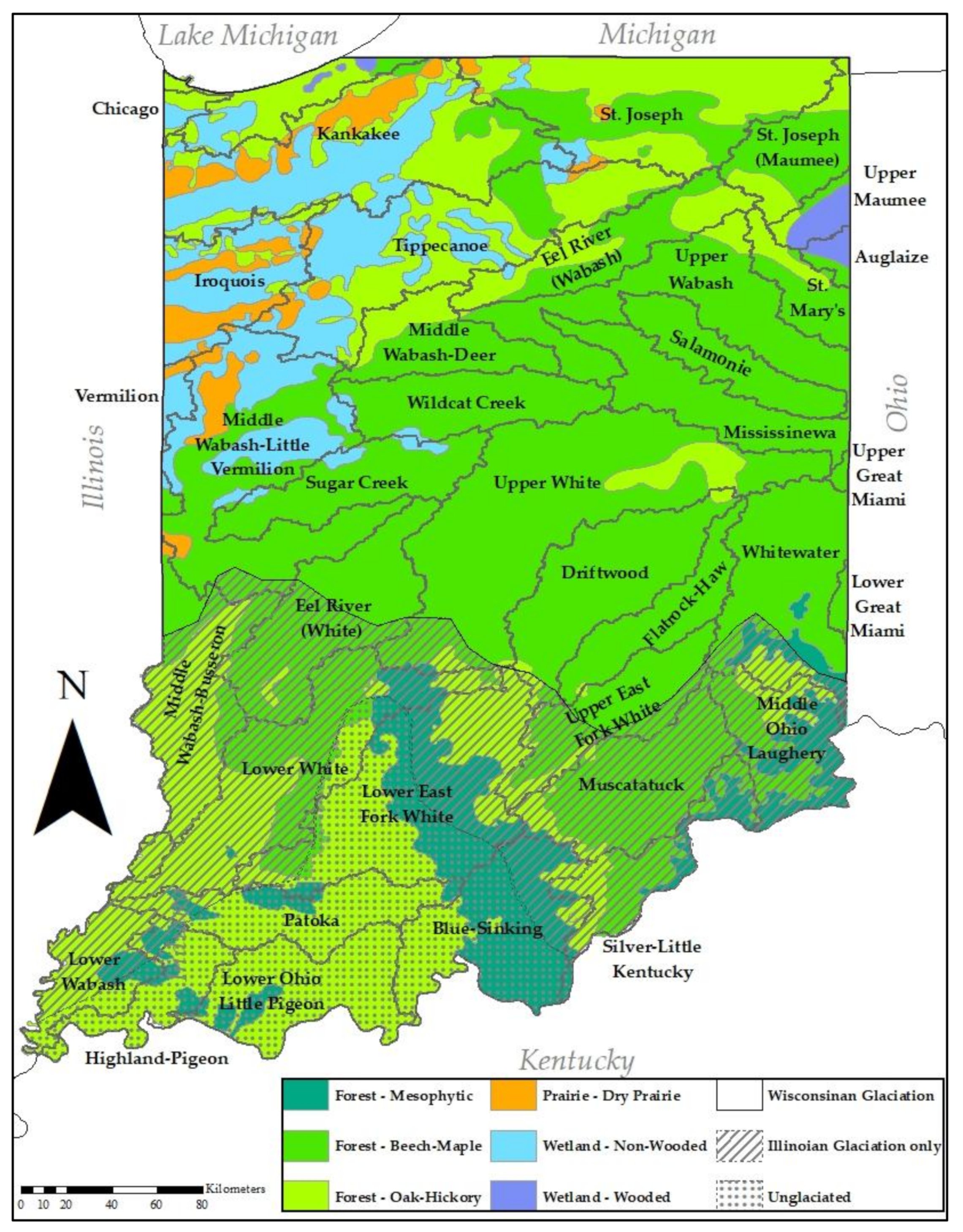
Present-day Indiana reflects two major glacial events [23,24]. The Illinoian glaciation, approximately 100,000 years ago at maximum extent, covered about 80% of Indiana. The Wisconsinan glaciation, maximum extent 18,000 years ago, covered approximately 60% (Figure 1, Table 1). These glacial events left three major landscapes within the state—the Wisconsinan (twice glaciated), the Illinoian (once glaciated), and the unglaciated south-central region. The Wisconsinan landscape is occupied by low-gradient streams and is deeply buried in glacial till. The older Illinoian landscape is eroded to abundant ravine streams and mature river valleys, and in the southwest along the Wabash River windblown loess ridges are common. Some larger river valleys of Illinoian age are filled with Wisconsinan-era outwash, forming large, meandering rivers. The unglaciated region is rugged with high-gradient streams, abundant groundwater, and exposed limestone bedrock.
The United States Geological Survey (USGS) hydrologic unit codes (HUCs) at the HUC8 scale [29] (Figure 1) were used as watershed replicates.
Prior to European settlement, Indiana supported six major vegetation communities—dry prairie, oak–hickory upland forest, beech–maple upland forest, beech–oak–maple–hickory mesophytic forest, wooded wetland, and non-wooded wetland [30,31,32,33] (Figure 1, Table 1). Forests dominated and prairies and wetlands occupied the northern third of Indiana. Currently, 62% of land use is agricultural (Table 2).
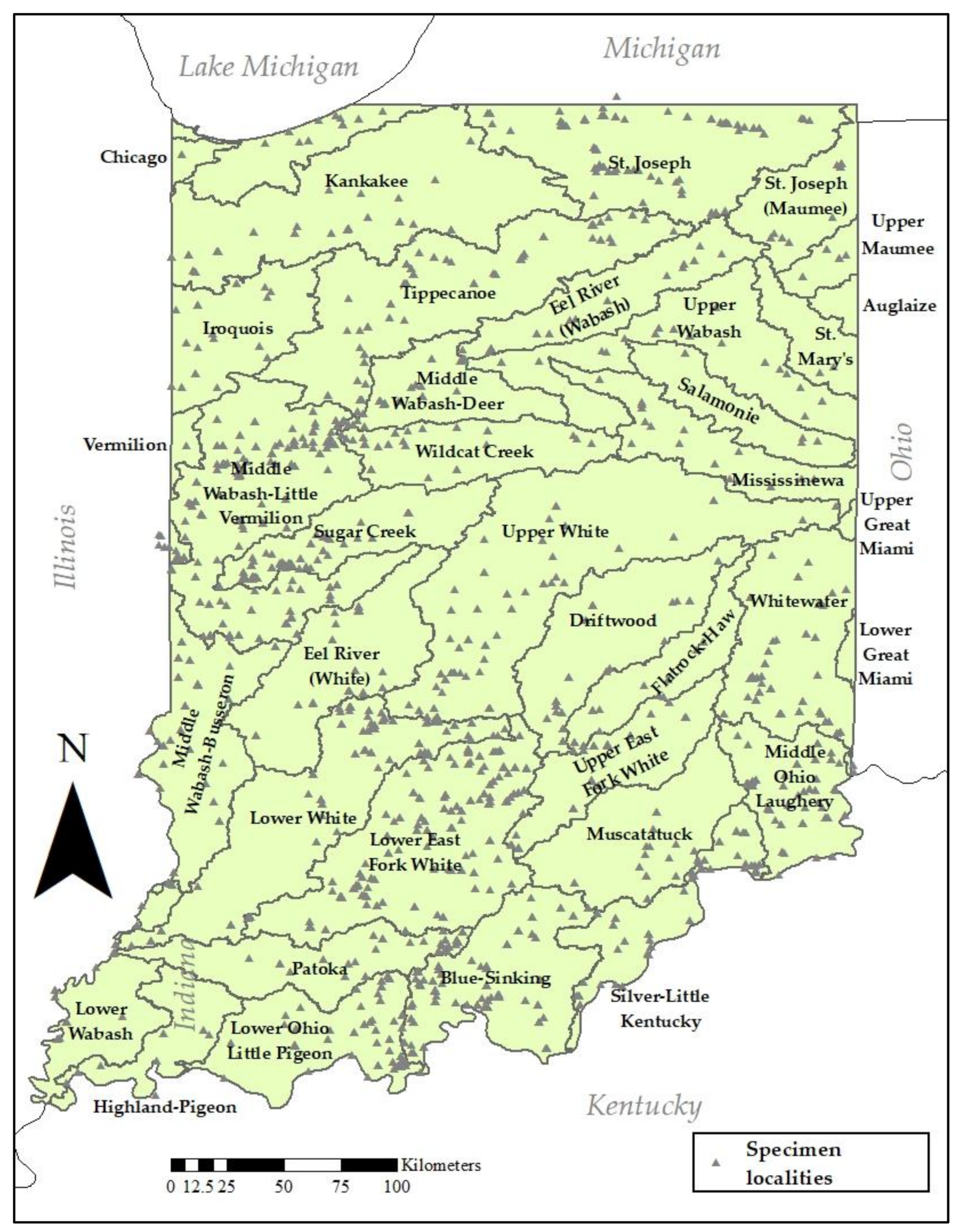
A large portion of the data used in this study resulted from examination of historical, borrowed specimens from many institutional and private collections, principal among these were the Illinois Natural History Survey Insect Collection (INHS), the Purdue University Entomological Research Collection (PERC), and the Western Kentucky University (WKUC). Sampling continued between 2000 and 2015 by DeWalt, Grubbs, and Donald W. Webb (deceased, INHS). Newman assumed lead of the project in 2016 and focused sampling on areas of the state where effort was sparse and rare species might be found. Throughout the century-long effort, sampling was not done at randomly selected locations, but was conducted at multiple locations within a full range of lotic habitats characteristic of the HUC8 being sampled (Figure 2). Resulting from this century of work is a highly detailed database of specimen and confirmed literature records. Historical and contemporary specimens were morphologically identified to the current state of the art. Recent literature used to identify species may be queried from the Plecoptera Species File Online [4]. Data from both larvae and adults were included where species-level identification was certain.
Border records were included in this analysis to increase the number of species within several Indiana peripheral drainages that were incompletely collected. These records met the following criteria for inclusion in the data set: the waterbody of the record formed a border with Indiana, or the locality of record was within 5 km of the state border and the same habitat existed in adjacent areas of Indiana. Border records were included from Illinois (110), Kentucky (3), Michigan (1), and Ohio (1).
Specimen data (locality labels, determination labels, and catalog numbers) were captured and normalized in a custom database. Most specimens were associated with their database record using a paper catalog number [34]. We georeferenced locations using an online mapping program [35] employing datum WGS-84. Where collectors provided coordinates, these were projected to verify the location and coordinates corrected accordingly. Precision of coordinates are provided as radius in meters: collector-provided = 10 m, localities with stream name and road crossing or small town name = 100–1000 m radius, localities with moderate population size to 50,000 people = 10,000 m, and Indiana county-level records = 100,000 m. State-level records were not mapped. County records were retained in analyses if drainage affiliation was certain.
Maps were exported from an ArcView 9.3 (ESRI) project file using a WGS-84 projection and overlaid on USGS HUC8 drainages. Each georeferenced record was thus assigned to a HUC8 drainage, allowing creation of a binary matrix of presence/absence of species by HUC8 drainage. Total species richness values were obtained from this matrix. Drainages with fewer than five recorded species were considered incompletely collected and were eliminated from analysis. Five species was the value for the Little Calumet drainage which was known to be well sampled [36]. Small drainages leaving or entering border states were trimmed to areas within Indiana.
All statistical analyses were conducted in an R environment [37]. Linear regression models were used to examine the relationship of species richness to the number of unique localities and HUC8 drainage area. This was accomplished using the lm function. The completeness of species discovery in Indiana was analyzed by building a species presence–absence vs. unique site-date collection events matrix. This matrix was used to fit a species accumulation curve using the specaccum function in vegan using 100 permutations [38]. Data were further subjected to the specpool function in order to estimate the species richness of the study area.
A K-means cluster analysis was used to examine the similarity of species assemblages between different drainages. The number of clusters represented by the data was determined using the “elbow method”, which indicated two clusters in the data. Jaccard distance between HUC8 species assemblages was calculated using vegdist function (vegan R package). This output was then subjected to hierarchical clustering using the hclust function (stats package). These data were plotted as a tree.
A natural and human disturbance variable set containing 116 environmental variables was assembled using three sources—USDA/NRCS Geospatial Gateway [39], USGS National Land Cover Database (NLCD) 2016 [40], and pre-European settlement vegetation from land survey data [32]. Variables fell into seven categories: climate, geology, hydrology, soils, topography, land cover, and historical ecosystem (vegetation).
Data from the USDA/NRCS and NLCD 2016 were in raster format while historical ecosystem data were formatted in shapefiles. All were treated similarly. Variables were extracted for each HUC8 drainage using ARCMap Spatial Analyst Tools, Zonal Statistics as Table to obtain a mean value for each HUC8. For datasets with several discrete values such as land cover, Spatial Analyst Tools, Tabulate Area was used and values were converted into percentages of coverage for each HUC8. Variable data were consolidated into a spreadsheet in Microsoft Excel (Microsoft, Redmond, WA, USA) for the first stage of variable reduction.
Multiple linear regression was used for variable set reduction followed by linear model-based variance partitioning to assess the effects of the environmental variables on Plecoptera species richness. Statistical methods for AIC based analyses were adapted from previous work [41].
To eliminate highly correlated variables, Pearson correlation coefficients were calculated. Pairs of variables were considered highly correlated if r ≥ 0.7. In this case, one variable was removed from further analysis based on interpretation and experience of which variable was likely more important to stonefly species richness. This reduced the number of variables by 75, leaving 41. The remaining variables were examined for variance inflation factor (VIF) in multiple linear regression modeling (vifstep in R package usdm). Variables with a VIF > 10 were considered highly collinear and were dropped from further analysis [41]. This left 15 variables which were tested for their effect on species richness using relative weights and dominance analysis. This procedure examines independent variable contribution to variance in a multiple linear regression model [42]. This was accomplished using the package yhat [43] using the function rlw. The relative weight values were used to reduce the 15 variable set to nine, as this is the maximum number that can be used in the hier.part function (package hier.part) used later in the analysis. Six of seven categories were represented by the remaining variables: hydrology, soils, land cover, historic ecosystem, HUC8 area, and geology (Table 3).
A generalized linear model was fit for species richness based on the remaining nine predictors using a Poisson distribution. The dispersion parameter was calculated as 1.64, negating the need for an over-dispersion adjustment to the data [37,41].
Using the dredge function in the R package MuMin [44,45], all possible candidate models using the variables from the global model were ranked using Akaike information criteria (AICc). Score differences in AICc (∆AICc) between the top-ranked model and all other models were used to select a group of models considered substantially supported [46]. Six models with a ∆AICc ≤ 2 were selected for further analysis. Model averaging was calculated for six well-supported models using R package AICcmodavg, using the modavg function. This method produced average coefficient estimates and 95% confidence intervals which were standardized to facilitate comparison of dissimilar variables [47]. Each predictor was assigned a relative importance value calculated by summing the model AICc weight of all models containing that particular variable. This analysis effectively eliminated % cherty red clay since it was not contained in any model where ∆AICc ≤ 2.
Further analysis was conducted using hierarchical variance partitioning, using the hier.part function in the hier.part R package [48]. Hierarchical variance partitioning estimates the percentage of variance explained by individual predictors in a linear model. This method compares all possible models in a multiple regression to obtain I, the measure of individual predictor effect on variance, and J, the contribution of a predictor when combined with each of the other predictors [49]. It provides another estimate of importance as confirmation of RIV importance, though they do not always agree. Data matrices of the top AICc importance predictors were randomized 1000 times with rand.hp to create distributions of I for each variable. Z-scores were computed with 95% confidence intervals for the value of I of each variable.
3. Results
3.1. Species Richness and Patterns
A total of 6339 specimen records were amassed during this study. Unique sampling events totalled 2411 and were conducted at 1050 unique locations from 1879 to 2021 (Figure 2). As a result, we recorded 93 stonefly species from Indiana (Table S1). Eight of 10 North American families were represented with Perlidae (36 species), Perlodidae (17), Capniidae (14), and Taeniopterygidae (7) providing 80% of all species collected in the state. No endemics were found, but four species represent new state records—Allocapnia pygmaea (Burmeister, 1839), Paracapnia angulata Hanson, 1961, Acroneuria lycorias (Newman, 1839), and an undescribed species, Perlesta IN-5 (temporary name).
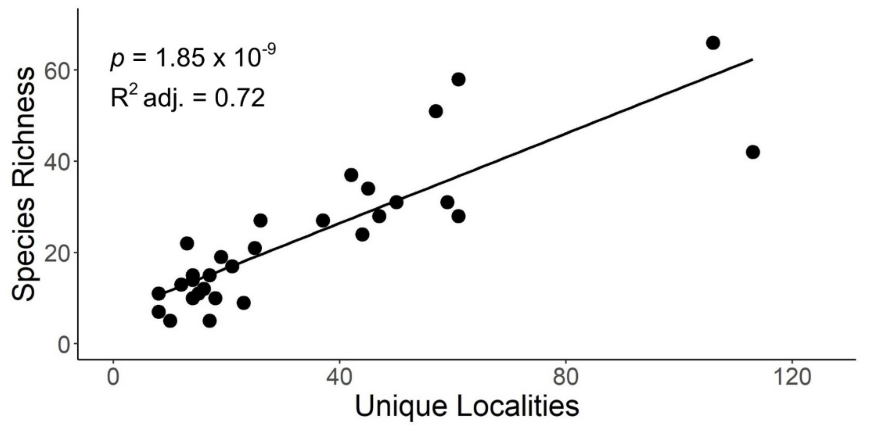
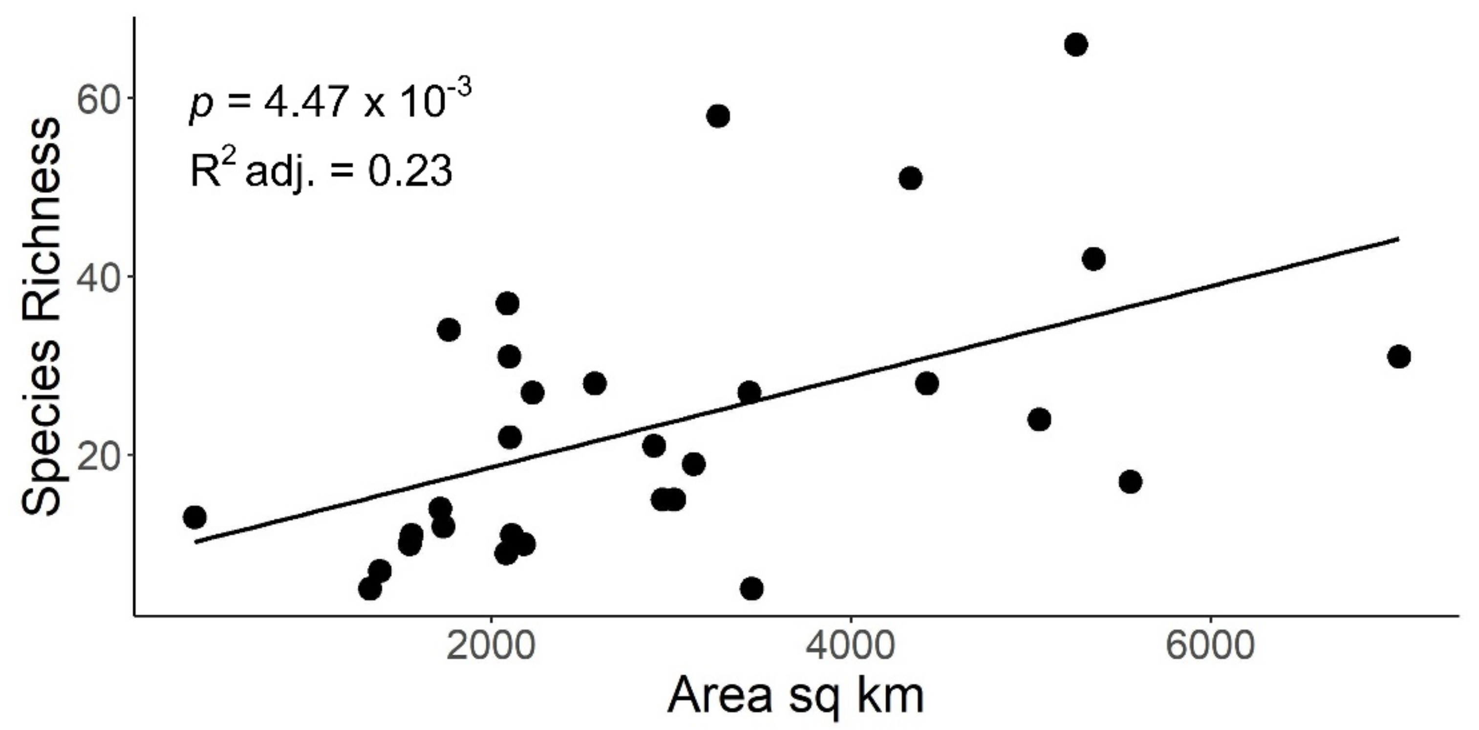
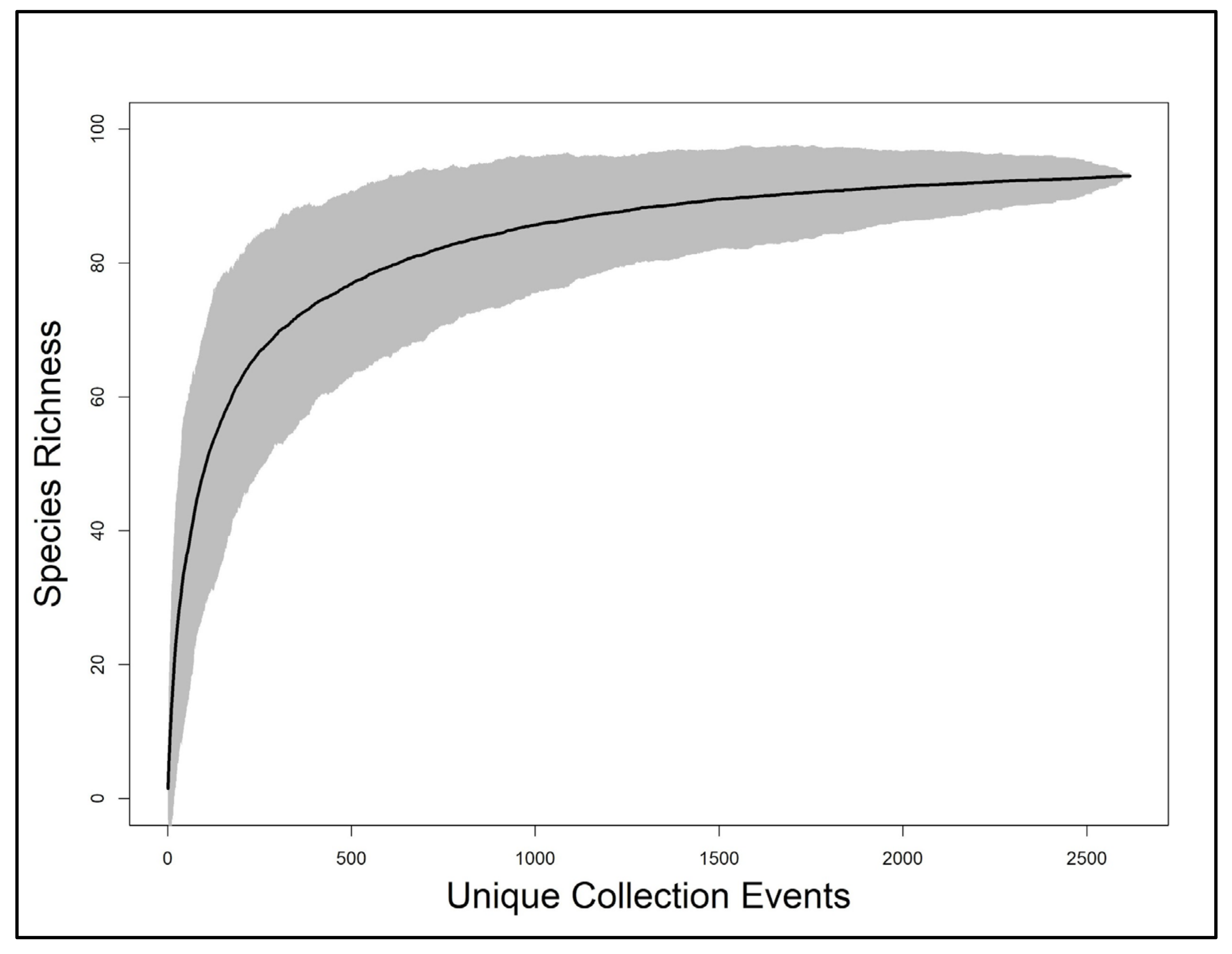
Linear regression indicated a significant, positive relationship between species richness and the number of unique localities sampled within HUC8 drainages (p = 1.85 × 10−09, adjusted R2 = 0.72) (Figure 3). Species richness demonstrated a significant, positive, but weaker relationship with HUC8 area (p-value: 0.005, adjusted R2 = 0.23) (Figure 4). A species accumulation curve demonstrates that stoneflies were sampled to near completeness (Figure 5). The model estimated a terminal species richness of 95 (±5) species, just two more than observed values.
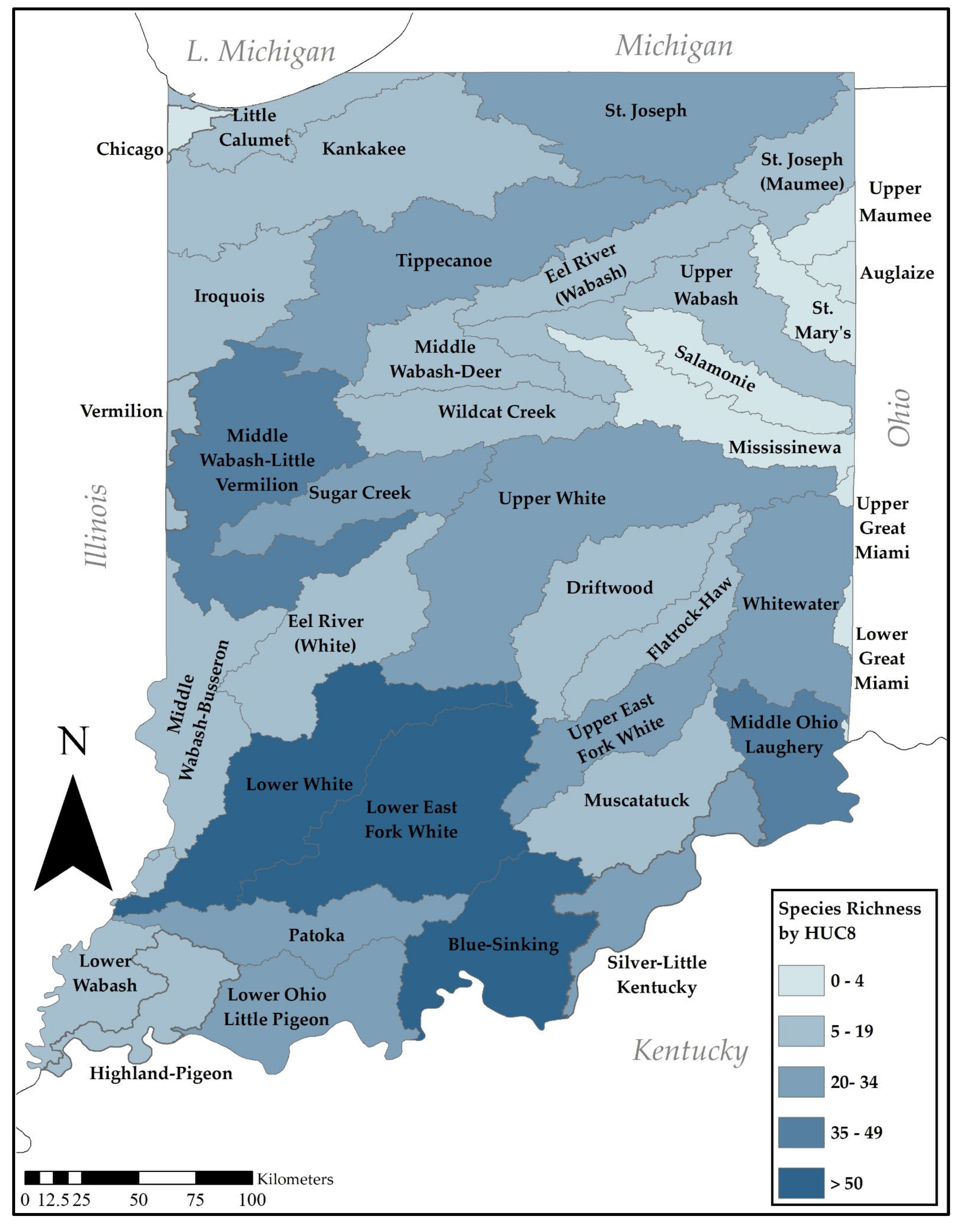
The mean number of species for the 30 HUC8 watersheds with five or more species was 23.3, with a median of 20.0. A heat map of species richness demonstrates that three hyperdiverse HUC8 drainages exist in Indiana (Figure 6, Table S2). These include the Lower East Fork White (66 species), the Blue-Sinking (58 species), and the Lower White (51 species), all in the southern third of the state. Other drainages with richness values above 30 species include the Middle Wabash–Little Vermilion (42 species), the Middle Ohio Laughery (37 species), Silver-L. Kentucky (34), Sugar Creek (31 species), and Upper White (31 species). These too occur in the southern half of the state. Eight watersheds were represented by four or fewer species, all were relatively small in drainage area, inadequately sampled, and unlikely to be diverse.
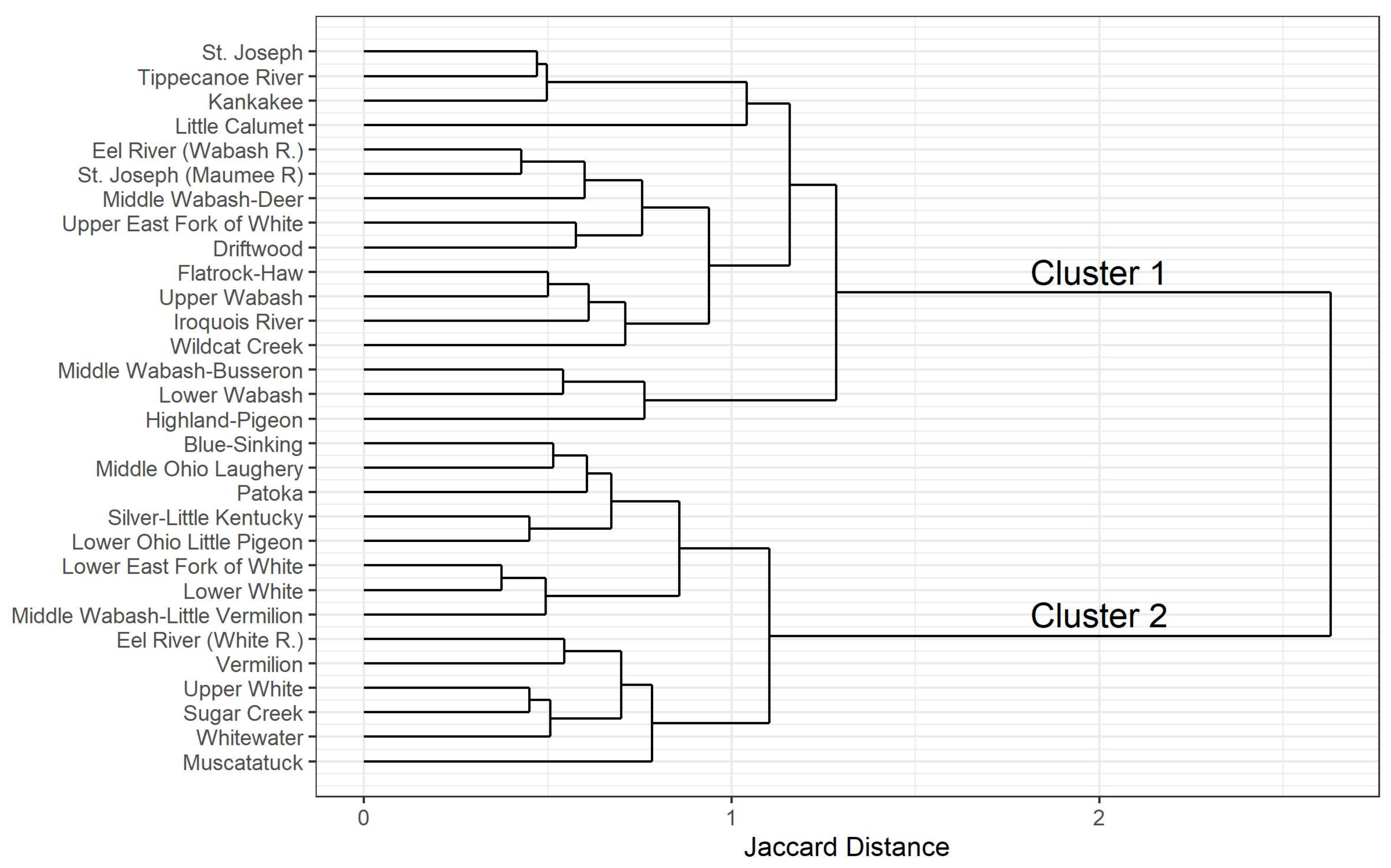
A K-means cluster analysis of HUC8 species assemblages produced two clusters. Cluster 1 contains drainages from the unglaciated and once-glaciated southern landscapes of Indiana (Figure 7). Cluster 2 is composed of mostly northern drainages with a few more large, southern drainages filled with glacial outwash.
3.2. Relative Importance of Watershed Variables in Species Richness
Analysis by AICc provided six models for species richness with ∆AICc ≤ 2 (Table 4). Akaike weights of these six models ranged from 0.0575 to 0.1548 with a mean of 0.0852 ± 0.0148 SE. McFadden R2 values suggest the models strongly explain variance in species richness and by a similar proportion among all models (McFadden R2 = 0.52–0.54 for top-six models). AICc analysis identified four variables included in all top-six models—mean topographic wetness index (TWI), area km2, % soils hydrogroup C/D, and % historic wetland ecosystem. Percent cherty red clay was the only variable not included in the ∆AICc ≤ 2 model set. All models contained between four and six variables. The best model, as determined by ΔAICc, was Model 1 with five variables (area, % soils hydrogroup CD, % development, % historic wetlands, and mean TWI), though all models were approximately equivalent.
Results of the AICc analysis were supported by standardized coefficients since none of the top-four variables contained zero within their 95% confidence intervals (Table 5). A positive predictor effect was found for three variables (area km2, % soils hydrogroup B, and % wetlands 2016) and the five remaining variables had a negative effect on species richness (% developed 2016, mean Horton overland flow, % historic wetland ecosystem, mean TWI, and % soils hydrogroup C/D).
AICc relative importance values (RIV) ranged from 0.196 to 1.000 (Figure 8). Relative positions of the top five variables were (1) mean TWI (1.00), (2) area km2 (1.00), (3) % soils hydrogroup C/D (0.91), (4) % historic wetland vegetation (0.88), and (5) % developed 2016 (0.62).
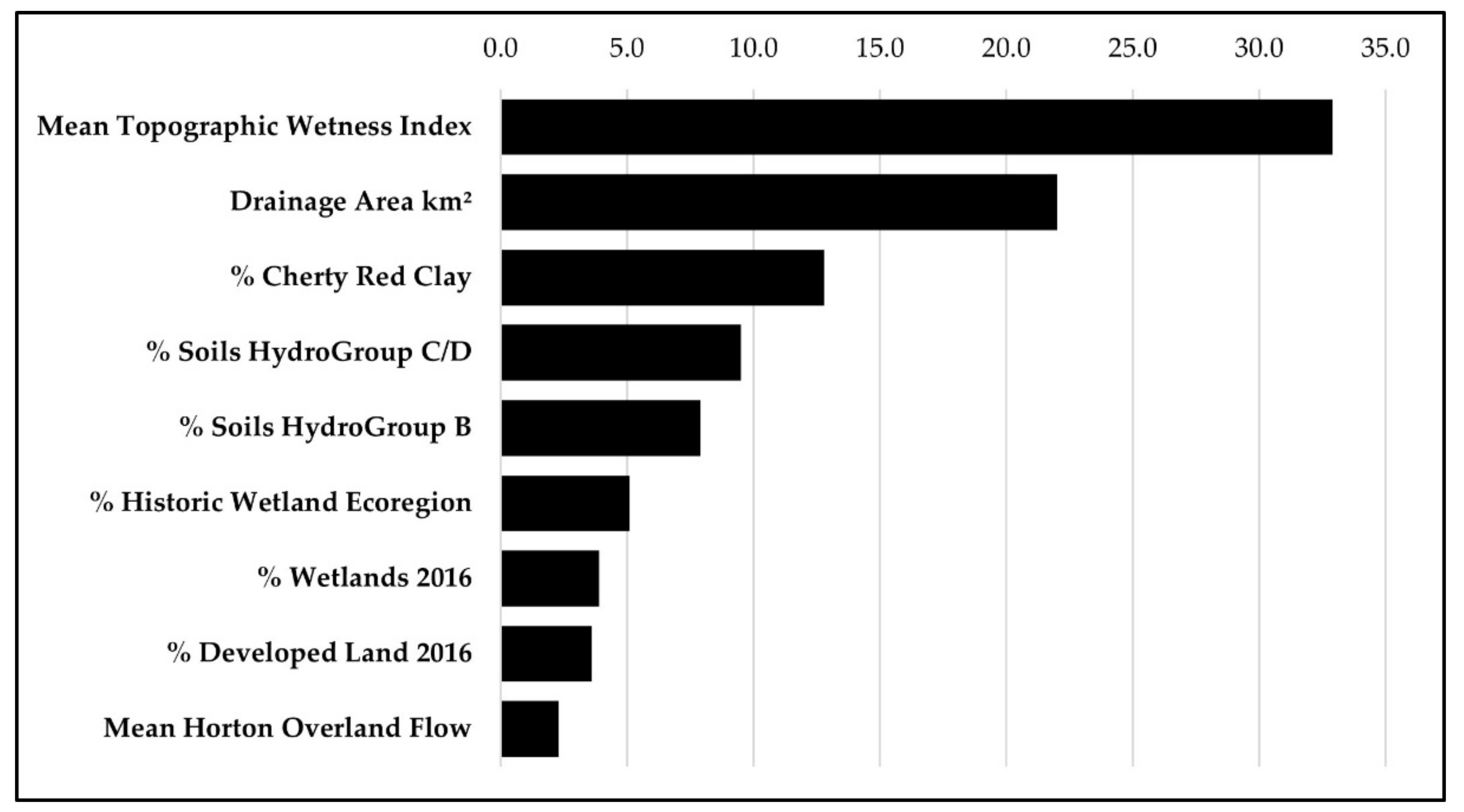
Relative positions of variables shifted when subjected to hierarchical partitioning. The relative positions of the top five highest scoring variables were (1) mean TWI (32.9%), (2) area km2 (22.0%), (3) % cherty red clay (12.8%), (4) % Soils hydrogroup CD (9.5%), and % Soils hydrogroup B (7.9%) (Figure 9). Percent cherty red clay was not included in any of the top six AIC models but ranked in the top three by hierarchical partitioning. Percent soils hydrogroup B moved above % historic wetland ecoregion. The other three variables in aggregate accounted for less than 10% variation.
Examining Z-scores indicated that mean TWI, area km2, and % cherty red clay, each explained a significant percentage of variance, with Z-scores over the 95% confidence limit (Figure 10).
4. Discussion
Large scale assessments of aquatic insect biodiversity are always difficult to conduct if species-level identification is needed. Sampling must be conducted instream for larvae and for adults in a wide variety of habitats and in multiple seasons; species succeed each other throughout the year [2]. In regions where water and habitat quality are degraded due to agricultural practices and human development many species will be missing or in distributions and densities too low for detection [10]. New sampling alone would not recover all species that were once present, nor would it produce natural ranges for species. Such is the case for Indiana, a midwestern USA state where at least 70% of land use is in agriculture and human development. Museum data are necessary to tally all species and to provide context for the species that still exist in an area. We have built a data set that allows us to recover the fauna of a highly disturbed landscape and ask questions about species richness of the entire assemblage of water and habitat quality sensitive species, how it is distributed across the landscape, and the relative importance of factors maintaining species richness.
4.1. Species Richness and Patterns
We recovered 93 species of stoneflies from Indiana, adding four species to the state tally [4]. Species richness was a positive function of unique sampling events and to a lesser degree by drainage area (Figure 3 and Figure 4). Both relationships were expected, though some heavily sampled drainages produced relatively few species. Our sampling nearly exhausted all species possible in the region (Figure 5) with a prediction being 95 ± 5 species. The current value of 93 is 14 more than known for Illinois [11]. Conversely, the new tally for Indiana is 9 fewer than Ohio’s 102 species [49] and 32 fewer than Kentucky [50]. Michigan has 68 species [12]. Regional tallies are known to be a function of both longitude and latitude, with decreases in species richness as both variables increase [13].
Indiana stonefly species richness is greatest in the southern part of the state, especially in HUC8s with large proportions of unglaciated area. The two richest HUC8s (Lower East Fork White, 66 and Blue-Sinking, 58) are largely unglaciated (Figure 6). The third-richest drainage (Lower White, 51 species) is an old, once-glaciated landscape, having been covered only by the Illinoisan glacial advance. These three drainages may have acted as a refuge during the Wisconsinan glaciation but were certainly first invaded from the Appalachian Mountains and plateaus east and south of the Ohio River [51].
A K-means cluster analysis of HUC8 assemblages suggests that there is substantial faunal turnover between northern and southern drainages (Figure 7). Cluster 1 drainages are mostly northern and of Wisconsinan glaciated landscapes. Cluster 2 is composed mainly of drainages from the southern half of Indiana in areas of Illinoian once-glaciated and unglaciated landscapes. The largest differences in the two clusters are within the winter- and spring-emerging Capniidae, Chloroperlidae, Leuctridae, Nemouridae, Perlodidae, and Taeniopterygidae. Cluster 1 contains 8 genera and 14 species, while Cluster 2 contains 21 genera and 52 species [4].
4.2. Relative Importance of Watershed Variables in Species Richness
AICc models 1–6 all explained 52–54% of the variation in species richness in drainages with only minor loss of information (Table 4). There is a pattern in the distribution of species richness within the HUC8 drainages. Four variables were always present in these six models: area km2, % soils hydrogroup CD, % historic wetland ecosystem, and TWI, all but one is related to hydrology. Examination of the importance of variables by RIV, %I contribution, and Z-scores always rated TWI and area km2 first and second. Ranking of other variables was inconsistent. One variable not found in the six models was % cherty red clay and it turned up the % I contribution of hierarchical partitioning and Z-scores in third position. Note that % developed 2016 appears to be unimportant in broad scale species richness of stoneflies in Indiana. All others are natural variables. This suggests that historical specimen data have helped to capture pre-European settlement stonefly assemblages.
TWI is a complex estimate of depth-to-water and had a negative relationship with Plecoptera species richness, i.e., areas with high TWI (marshes and wooded wetlands) supported lower species richness (as in the Little Calumet drainage). Conversely, low TWI values indicate areas that drain well, have higher slopes, coarser substrates, and higher dissolved oxygen values. These are conditions conducive to stonefly species richness (as in the high richness Lower East Fork White and Blue-Sinking drainages). Some studies used TWI as a predictive measure for the presence of wetlands [52]. Others found a negative relationship of TWI with understory vegetation species richness in an Alberta, Canada boreal forest, i.e., drier habitats had greater species richness than wetter ones [53]. Conversely, an assemblage of grassland-inhabiting passerine birds living in the floodplain of the Loire valley, France was positively associated with TWI [54].
HUC8 area km2 was the second most important variable and a positive predictor of species richness. Larger HUC8s contain a diversity of habitat types (seeps, ravine streams, and medium and large streams), supporting greater species richness. In Ohio, no relationship between drainage area and species richness of stoneflies was found [13], but the analysis was based on the much larger HUC6-scale drainages which may have smoothed habitat differences between drainages. Several other large-scale analyses of aquatic insect distributions have been conducted, but none have analyzed the effect of drainage area on species richness: for stoneflies [55] and caddisflies [56] in the Ozark and Ouachita Mountains area and for caddisflies in Minnesota [57]. Also working in the Ozark/Ouachita/Interior Highlands area, drainage area accounted for approximately 35% of variance in species richness of native fish [58]. Their drainages approximated HUC8 to HUC12 scale.
The third-most important variable in AICc and fourth in hierarchical partitioning was % soils in hydrogroup C/D (I = 9.5%). Soils in hydrologic group C/D are notoriously slow-draining [59]. In Indiana, these soils are common in large river bottoms in the southern half of the state, but they make up a large proportion of soils in the Eel (Wabash), Mississinewa, Salamonie, Upper Wabash, St. Joseph (Maumee), St. Mary’s, Maumee, and Auglaize drainages where five under-sampled drainages were eliminated from the analysis. This region makes up the Bluffton Till Plain [31,33]. The soils were largely formed by precursors of Lake Erie and deposited by minor re-advances of glaciers, leaving a series of concentric moraines that divide the HUC8s of this region. Others [12,50] reported similar results of low stonefly richness for adjacent drainages in northwest Ohio. This hydrologic soil group is a representation of permeability and a function of the least transmissive horizon of soil in a location [59]. They may be placed in a dual category if the water table is present within 60 cm of the surface, even if the soil makeup is conducive to faster draining. This is the case of our % hydrologic group C/D. These are sandy clay loams where the water table is naturally within 60 cm of the surface.
Percent historic wetland ecosystem is likely representing a similar impact, though from a different part of the state. The lower portion of the Maumee and its tributaries in Indiana were wetlands, part of the Great Black Swamp, a wooded wetland complex formed atop lake plains of ancient glacial Lake Maumee [60]. Additionally, other major wetland complexes were found in northwestern Indiana as part of the Grand Kankakee Marsh and drained by the Calumet, Kankakee, Iroquois, Tippecanoe, and Middle Wabash–Little Vermilion drainages [30]. This is also the region where most of the state’s wet and dry prairies occurred, which were grouped together with other emergent wetlands in presettlement vegetation percentages [35]. These areas are rich in flat streams with low gradients and sandy soils. Few stoneflies live in such conditions [36].
Percent cherty red clay was not included in AICc importance since it was not included in any of the top six models where ∆AICc ≤ 2. However, it ranked third with a positive relationship to richness when the dataset was subjected to hierarchical partitioning and Z-scores. This category of surface geology is associated with unglaciated Indiana [30]. Cherty red clay is a surface geology in portions of six HUC8 drainages, but it only makes up >5% area in three (Blue-Sinking, 70.0%; Lower East Fork White, 39.7%; and Silver-Little Kentucky, 11.3%). Eroding from these soils are chert nodules, biologically formed inclusions found in limestone. The presence of chert indicates moderate and high slopes, coarse substrates, and groundwater influence, all important for supporting high stonefly species richness. This variable appears important in only a small area of Indiana. It may be a more important variable in unglaciated areas where limestone is more extensively distributed.
It is important to note that Plecoptera species richness differs greatly across the drainages of the state. The top four most species-rich HUC8s are the Lower East Fork White (66 species), the Blue-Sinking (58), the Lower White (51), and the Middle Wabash–Little Vermilion (42) and they greatly exceed the mean value of 23.3 species. It should also be noted that certain lower-scoring HUC8s greatly outperform their neighbors. The St. Joseph River, which drains to Lake Michigan, still supports a nearly complete assemblage of large perlid and perlodid stoneflies: Acroneuria (three species), Agnetina (one species), Paragnetina (one species), Neoperla (one species), Isoperla (three species). This number is approximately twice as many species as found in adjacent HUC8s to the east and south. Morainal systems in this drainage created a more varied topography, swifter current, glacial lakes, and abundant groundwater.
5. Conclusions
Our results highlight the importance of hydrology on species richness of Plecoptera. Three of the top four variables in AICc importance are directly tied to hydrology—TWI, % soils in hydrogroup C/D, and % historic wetlands. These factors are important in that they reflect available substrates, water availability, flow rate, and dissolved oxygen. Human disturbance variables were unimportant in explaining HUC8 diversity.
We could not directly demonstrate the importance of glacial history to Indiana Plecoptera species richness, but several of the hydrology variables are likely surrogates for glacial history. Percent cherty red clay may also be indicative of lack of glaciation. The cluster analysis strongly suggests a role for glacial history.
Land use over the past two centuries has had a significant impact on current species richness across the state [11]. This study tallies species present in museum records dating back to 1879. The older records place many species in drainages where they no longer occur [10,11]. Eight stonefly species have not been collected in Indiana since the early- to mid-20th century. These species primarily inhabited large rivers, especially the middle and lower Wabash and lower White rivers. The timing of these extirpations correlates with the change to mechanized agriculture and the use of chemical insecticides, herbicides, and fertilizers [9]. Currently, 62% of the land area of Indiana is in agriculture, and Wisconsinan glaciated areas share an outsized proportion of land devoted to agriculture. High stonefly species richness persists only in unglaciated and once-glaciated areas where topography is not conducive to widespread agriculture [10].
The work conducted here is of sufficient extent and intensity that additional analyses are possible. A distributional atlas of all the stoneflies species in Indiana is nearly ready for submission. Conservation status assessments with these data are also planned for early 2022. The latter will help inform conservation efforts of species, important drainages, and individual waterbodies. It has taken the efforts of many scientists over the past century to gather these data.
Indiana data and those of a seven state region are now being used to predict pre-European distribution of stoneflies throughout the wider Midwest, USA. This will be the precursor for predicting future distributions as influenced by climate and other variables.
Supplementary Materials
The following are available online at https://0-www-mdpi-com.brum.beds.ac.uk/article/10.3390/d13120672/s1, Table S1: Presence/absence data matrix for Indiana stoneflies (Plecoptera) and USGS HUC8 drainages they occur within. Genus included where the species was undeterminable but present in the HUC8, Table S2: USGS HUC8 watersheds, HUC8 code, species richness, number of specimen records, and drainage area.
Author Contributions
Conceptualization, E.A.N., R.E.D. and S.A.G.; methodology, E.A.N. and R.E.D.; formal analysis, E.A.N.; data curation, E.A.N.; writing—original draft preparation, E.A.N. and R.E.D.; writing—review and editing, E.A.N., R.E.D. and S.A.G.; supervision, R.E.D.; project administration, R.E.D.; funding acquisition, R.E.D. All authors have read and agreed to the published version of the manuscript.
Funding
The USA National Science Foundation, grant number CSBR 14-58285 funded a graduate research assistantship and tuition for E.A.N. NSF DEB 09-18805 ARRA and USA Fish and Wildlife Service DOI-USFWS X-1-R-1 funded accumulation of specimen data. The Indiana Department of Natural Resources and the Indianapolis Zoo grant number 0017556043 funded a status assessment of stoneflies. The University of Illinois, Department of Entomology and the Society for Freshwater Science Conservation grant competition provided summer travel grants to E.A.N. for this project. The International Society of Plecopterologists provided generous travel funds to E.A.N. to present at an international meeting.
Institutional Review Board Statement
Not applicable.
Informed Consent Statement
Not applicable.
Data Availability Statement
Most specimen data used in this study are available from the INHS Insect Collection database portal at http://inhsinsectcollection.speciesfile.org/InsectCollection.aspx (Accessed on 13 December 2021). These data are also replicated at the Global Biodiversity Information Facility portal at https://www.gbif.org/ (Accessed on 13 December 2021). Museum data from PERC are held in a private database that will soon become available through GBIF. We have provided all data to the Indiana Department of Natural Resources as a deliverable.
Acknowledgments
We thank Arwin Provonsha, former collection manager at the Purdue University Entomological Research Collection, who, over a decade, gave us access to and provided loans of stonefly specimens. Permits (NP20-05) to sample Indiana state properties were facilitated by Ronald P. Hellmich, Director, Division of Nature Preserves, Indiana Department of Natural Resources. We are grateful to Jason L. Robinson (INHS) for digitizing the pre-European settlement vegetation data.
Conflicts of Interest
The authors declare no conflict of interest. The funders had no role in the design of the study; in the collection, analyses, or interpretation of data; in the writing of the manuscript, or in the decision to publish the results.
References
- Fochetti, R.; Tierno de Figueroa, J.M. Global diversity of stoneflies (Plecoptera; Insecta) in freshwater. Hydrobiologia 2008, 595, 365–377. [Google Scholar] [CrossRef]
- DeWalt, R.E.; Kondratieff, B.C.; Sandberg, J.B. Order Plecoptera. In Ecology and General Biology: Thorp and Covich’s Freshwater Invertebrates; Thorp, J., Rogers, D.C., Eds.; Academic Press: Cambridge, MA, USA, 2015; pp. 933–949. ISBN 9780123850263. [Google Scholar]
- DeWalt, R.E.; Ower, G.D. Ecosystem services, global diversity, and rate of stonefly species descriptions (Insecta: Plecoptera). Insects 2019, 10, 99. [Google Scholar] [CrossRef] [PubMed] [Green Version]
- DeWalt, R.E.; Maehr, M.D.; Hopkins, H.; Neu-Becker, U.; Stueber, G.; Plecoptera Species File Online. Version 5.0/5.0. 2021. Available online: http://Plecoptera.SpeciesFile.org (accessed on 25 October 2021).
- South, E.J.; Skinner, R.K.; DeWalt, R.E.; Davis, M.A.; Johnson, K.P.; Teslenko, V.A.; Lee, J.J.; Malison, R.L.; Hwang, J.M.; Bae, Y.J.; et al. A new family of stoneflies (Insecta: Plecoptera), Kathroperlidae, fam. n., with a phylogenomic analysis of the Paraperlinae (Plecoptera: Chloroperlidae). Insect Syst. Divers. 2021, 5, 1. [Google Scholar] [CrossRef]
- Barbour, M.T.; Gerritsen, J.; Snyder, B.D.; Stribling, J.B. Rapid Bioassessment Protocols for Use in Streams and Wadeable Rivers: Periphyton, Benthic Macroinvertebrates and Fish, 2nd ed.; U.S. Environmental Protection Agency Office of Water: Washington, DC, USA, 1999. [Google Scholar]
- Lenat, D.R. A biotic index for the southeastern United States: Derivation and list of tolerance values, with criteria for assigning water-quality ratings. J. N. Am. Benthol. Soc. 1993, 12, 279–290. [Google Scholar] [CrossRef]
- Shah, D.N.; Domisch, S.; Pauls, S.U.; Haase, P.; Jähnig, S.C. Current and future latitudinal gradients in stream macroinvertebrate richness across North America. Freshw. Sci. 2014, 33, 1136–1147. [Google Scholar] [CrossRef]
- Master, L.L.; Stein, B.A.; Kutner, L.S.; Hammerson, G.A. Vanishing assets: Conservation status of U.S. species. In Precious Heritage: The Status of Biodiversity in the United States; Stein, B.A., Kutner, L.S., Adams, J.S., Eds.; The Oxford University Press: New York, NY, USA, 2000; pp. 93–118. [Google Scholar]
- DeWalt, R.E.; Favret, C.; Webb, D.W. Just how imperiled are aquatic insects? A case study of stoneflies (Plecoptera) in Illinois. Ann. Entomol. Soc. Am. 2005, 98, 941–950. [Google Scholar] [CrossRef]
- DeWalt, R.E.; Grubbs, S.A. Updates to the Stonefly Fauna of Illinois and Indiana. Illiesia 2011, 7, 31–50. [Google Scholar]
- Grubbs, S.A.; Pessino, M.; DeWalt, R.E. Michigan Plecoptera (Stoneflies): Distribution patterns and an updated species list. Illiesia 2012, 8, 162–173. [Google Scholar]
- DeWalt, R.E.; Cao, Y.; Tweddale, T.; Grubbs, S.A.; Hinz, L.; Pessino, M.; Robinson, J.L. Ohio USA stoneflies (Insecta, Plecoptera): Species richness estimation, distribution of functional niche traits, drainage affiliations, and relationships to other states. ZooKeys 2012, 178, 1–26. [Google Scholar] [CrossRef] [Green Version]
- Grubbs, S.A.; Pessino, M.; DeWalt, R.E. Distribution patterns of Ohio stoneflies, with an emphasis on rare and uncommon species. J. Insect Sci. 2013, 13, 72. [Google Scholar] [CrossRef]
- Bojková, J.; Komprdová, K.; Soldán, T.; Zahrádková, S. Species loss of stoneflies (Plecoptera) in the Czech Republic during the 20th century. Freshw. Biol. 2012, 57, 2550–2567. [Google Scholar] [CrossRef]
- Sánchez-Bayo, F.; Wyckhuys, K.A.G. Worldwide decline of the entomofauna: A review of its drivers. Biol. Conserv. 2019, 232, 8–27. [Google Scholar] [CrossRef]
- Zwick, P. Stream habitat fragmentation—A threat to biodiversity. Biod. Conserv. 1992, 1, 80–97. [Google Scholar] [CrossRef]
- Pires, M.M.; Grech, M.G.; Stenert, C.; Maltchik, L.; Epele, L.B.; McLean, K.I.; Kneitel, J.M.; Bell, D.A.; Greig, H.S.; Gagne, C.R.; et al. Does taxonomic and numerical resolution affect the assessment of invertebrate community structure in New World freshwater wetlands? Ecol. Indic. 2021, 125, 107437. [Google Scholar] [CrossRef]
- Lenat, D.R.; Resh, V.H. Taxonomy and stream ecology—The benefits of genus and species-level identifications. J. N. Am. Benthol. Soc. 2001, 20, 287–298. [Google Scholar] [CrossRef]
- Needham, J.G.; Claassen, P.W. A Monograph of the Plecoptera or Stoneflies of America North of Mexico; The Thomas Say Foundation: Lafayette, IN, USA, 1925; Volume 11, 397p. [Google Scholar]
- Frison, T.H. Fall and winter stoneflies, or Plecoptera, of Illinois. Ill. Nat. Hist. Surv. Bull. 1929, 18, 344–409. [Google Scholar] [CrossRef]
- Frison, T.H. The stoneflies, or Plecoptera, of Illinois. Ill. Nat. Hist. Surv. Bull. 1935, 20, 281–467. [Google Scholar] [CrossRef]
- Frison, T.H. Studies of North American Plecoptera with special reference to the fauna of Illinois. Ill. Nat. Hist. Surv. Bull. 1942, 22, 233–355. [Google Scholar]
- Ricker, W.E. A first list of Indiana stoneflies (Plecoptera). Proc. Indiana Acad. Sci. 1945, 54, 225–230. [Google Scholar]
- Bednarik, A.F.; McCafferty, W.P. A checklist of the stoneflies, or Plecoptera, of Indiana. Great Lakes Entomol. 1977, 10, 223–226. [Google Scholar]
- Grubbs, S.A. Studies on Indiana stoneflies (Plecoptera), with an annotated and revised state checklist. Proc. Entomol. Soc. Wash. 2004, 106, 865–876. [Google Scholar]
- Grubbs, S.A.; DeWalt, R.E. Perlesta ephelida, a new Nearctic stonefly species (Plecoptera: Perlidae). ZooKeys 2012, 194, 1–15. [Google Scholar] [CrossRef] [Green Version]
- Grubbs, S.A.; DeWalt, R.E. Perlesta armitagei n. sp. (Plecoptera: Perlidae): More cryptic diversity in darkly pigmented Perlesta from the eastern Nearctic. Zootaxa 2018, 4442, 83–100. [Google Scholar] [CrossRef] [PubMed]
- Hydrologic Unit Maps. Available online: https://water.usgs.gov/GIS/huc.html (accessed on 1 January 2021).
- Malott, C.A. The physiography of Indiana. In Handbook of Indiana Geology; Indiana Department of Conservation Publication; William B. Burford, Contractor for State Printing and Binding: Indianapolis, IN, USA, 1922; Volume 21, pp. 59–256. [Google Scholar]
- Gray, H.H. Physiographic Divisions of Indiana; Indiana Geological Survey Special Report 61; Indiana Geological and Water Survey: Bloomington, IN, USA, 2000; 15p. [Google Scholar]
- Lindsey, A.A.; Crankshaw, W.B.; Qadir, S.A. Soil relations and distribution map of the vegetation of presettlement Indiana. Bot. Gaz. 1965, 126, 155–163. [Google Scholar] [CrossRef]
- Homoya, M.A.; Abrell, D.B.; Aldrich, J.R.; Post, T.W. The Natural Regions of Indiana. Proc. Indiana Acad. Sci. 1985, 94, 245–268. [Google Scholar]
- DeWalt, R.E.; Yoder, M.; Snyder, E.; Dmitriev, D.; Ower, G. Wet collections accession: A workflow based on a large stonefly (Insecta, Plecoptera) donation. Biodivers. Data J. 2018, 6, e30256. [Google Scholar] [CrossRef] [PubMed]
- Acme Mapper 2.2. Available online: http://mapper.acme.com (accessed on 28 October 2021).
- DeWalt, R.E.; South, E.J.; Robertson, D.R.; Marburger, J.E.; Smith, W.W.; Brinson, V. Mayflies, stoneflies, and caddisflies of streams and marshes of Indiana Dunes National Lakeshore, USA. ZooKeys 2016, 556, 43–63. [Google Scholar] [CrossRef] [PubMed]
- R Core Team. R: A Language and Environment for Statistical Computing; R Foundation for Statistical Computing: Vienna, Austria, 2014; Available online: http://www.R-project.org/ (accessed on 1 January 2021).
- Oksanen, J.; Blanchet, F.G.; Friendly, M.; Kindt, R.; Legendre, P.; McGlinn, D.; Minchin, P.R.; O’Hara, R.B.; Simpson, G.L.; Solymos, P.; et al. Vegan: Community Ecology Package, R Rackage Version 2.5-7; R Project for Statistical Computing: Vienna, Austria, 2020; Available online: https://CRAN.R-project.org/package=vegan (accessed on 1 January 2021).
- Geospatial Data Gateway. Available online: https://datagateway.nrcs.usda.gov/ (accessed on 1 January 2021).
- Wickham, J.; Stehman, S.V.; Sorenson, D.G.; Gass, L.; Dewitz, J.A. Thematic accuracy assessment of the NLCD 2016 land cover for the conterminous United States. Remote Sens. Environ. 2021, 257, 112357. [Google Scholar] [CrossRef]
- South, E.J.; DeWalt, R.E.; Cao, Y. Relative importance of Conservation Reserve Programs to aquatic insect biodiversity in an agricultural watershed in the Midwest, USA. Hydrobiologia 2019, 829, 323–340. [Google Scholar] [CrossRef]
- Quinn, G.P.; Keough, M.J. Experimental Design and Data Analysis for Biologists; Cambridge University Press: New York, NY, USA, 2002. [Google Scholar]
- Budescu, D.V. Dominance analysis: A new approach to the problem of relative importance of predictors in multiple regression. Psychol. Bull. 1993, 114, 542–551. [Google Scholar] [CrossRef]
- Nimon, K.; Oswald, F.; Roberts, J.K. Yhat: Interpreting Regression Effects, R Package Version 2.0-0; R Project for Statistical Computing: Vienna, Austria, 2021; Available online: https://CRAN.R-project.org/package=yhat (accessed on 15 January 2021).
- Burnham, K.P.; Anderson, D.R. Model Selection and Multimodel Inference: A Practical Information-Theoretic Approach, 2nd ed.; Springer: New York, NY, USA, 2002. [Google Scholar]
- Barton, K. MuMIn: Multi-Model Inference; R package Version 1.15.1; R Project for Statistical Computing: Vienna, Austria, 2015. [Google Scholar]
- Burnham, K.P.; Anderson, D.R. Multimodel inference: Understanding AIC and BIC in model selection. Sociol. Methods Res. 2004, 33, 261–304. [Google Scholar] [CrossRef]
- Chevan, A.; Sutherland, M. Hierarchical partitioning. Am. Stat. 1991, 45, 90–96. [Google Scholar] [CrossRef]
- DeWalt, R.E.; Grubbs, S.A.; Armitage, B.; Baumann, R.W.; Clark, S.M.; Bolton, M.J. Atlas of Ohio Aquatic Insects: Volume II, Plecoptera. Biodivers. Data J. 2016, 4, e10723. [Google Scholar] [CrossRef] [Green Version]
- Tarter, D.C.; Chaffee, D.L.; Grubbs, S.A.; DeWalt, R.E. New state records of Kentucky (USA) stoneflies (Plecoptera). Illiesia 2015, 11, 167–174. [Google Scholar]
- Pessino, M.; Chabot, E.T.; Giordano, R.; DeWalt, R.E. Refugia and postglacial expansion of Acroneuria frisoni Stark & Brown (Plecoptera: Perlidae) in North America. Freshw. Sci. 2014, 33, 232–249. [Google Scholar] [CrossRef]
- Ganser, C.; Wisely, S.M. Patterns of spatio-temporal distribution, abundance, and diversity in a mosquito community from the eastern Smoky Hills of Kansas. J. Vector Ecol. 2013, 38, 229–236. [Google Scholar] [CrossRef]
- Echiverri, L.; MacDonald, S.E. Utilizing a topographic moisture index to characterize understory vegetation patterns in the boreal forest. For. Ecol. Manag. 2019, 447, 35–52. [Google Scholar] [CrossRef]
- Besnard, A.G.; La Jeunesse, I.; Pays, O.; Secondi, J. Topographic wetness index predicts the occurrence of bird species in floodplains. Divers. Distrib. 2013, 19, 955–963. [Google Scholar] [CrossRef]
- Poulton, B.C.; Stewart, K.W. The stoneflies of the Ozark and Ouachita Mountains (Plecoptera). Mem. Am. Entomol. Soc. 1991, 38, 1–116. [Google Scholar]
- Moulton, S.R., II; Stewart, K.W. Caddisflies (Trichoptera) of the Interior Highlands of North America. Mem. Am. Entomol. Inst. 1996, 56, 1–313. [Google Scholar]
- Houghton, D.C. Biological diversity of the Minnesota caddisflies (Insecta, Trichoptera). ZooKeys 2012, 189, 1–389. [Google Scholar] [CrossRef]
- Matthews, W.J.; Robison, H.W. Influence of drainage connectivity, drainage area and regional species richness on fishes of the Interior Highlands in Arkansas. Am. Midl. Nat. 1998, 139, 1–19. [Google Scholar] [CrossRef]
- United States Soil Conservation Service. Hydrologic Soil Groups. In National Engineering Handbook; Section 630, Chapter 7; United States Department of Agriculture: Washington, DC, USA, 2007. [Google Scholar]
- Kaatz, M. The Black Swamp: A study in historical geography. Ann. Assoc. Am. Geogr. 1955, 45, 1–35. [Google Scholar] [CrossRef]
Figure 1.
Map of Indiana vegetation prior to European settlement and glaciation. Adapted from Lindsey et al. [32].
Figure 1.
Map of Indiana vegetation prior to European settlement and glaciation. Adapted from Lindsey et al. [32].

Figure 2.
Map of Plecoptera specimen localities in Indiana.

Figure 3.
Scatterplot of stonefly species richness versus the unique localities within HUC8 watersheds of Indiana. Adjusted R2, probability, and line of best fit provided for simple linear regression analysis.
Figure 3.
Scatterplot of stonefly species richness versus the unique localities within HUC8 watersheds of Indiana. Adjusted R2, probability, and line of best fit provided for simple linear regression analysis.

Figure 4.
Scatterplot of stonefly species richness versus Indiana HUC8 watershed drainage area in km2. Adjusted R2, probability, and line of best fit provided for simple linear regression analysis.
Figure 4.
Scatterplot of stonefly species richness versus Indiana HUC8 watershed drainage area in km2. Adjusted R2, probability, and line of best fit provided for simple linear regression analysis.

Figure 5.
Species accumulation curve with 95% confidence interval (gray shade) for Indiana Plecoptera using unique collection events as replicates. Terminal estimation was 95 ± 5 species.
Figure 5.
Species accumulation curve with 95% confidence interval (gray shade) for Indiana Plecoptera using unique collection events as replicates. Terminal estimation was 95 ± 5 species.

Figure 6.
Heat map of Plecoptera species richness within HUC8 watersheds in Indiana.

Figure 7.
Hierarchical cluster tree based on K-means analysis of species by HUC8 drainage.

Figure 8.
AICc Relative Importance Values (RIV) for nine variables included in the global model.

Figure 9.
The %I contribution to variance in species richness determined by hierarchical partitioning.
Figure 9.
The %I contribution to variance in species richness determined by hierarchical partitioning.

Figure 10.
Z-scores of variables determined by hierarchical partitioning. * Denotes variables significant at 95% confidence interval.
Figure 10.
Z-scores of variables determined by hierarchical partitioning. * Denotes variables significant at 95% confidence interval.


Table 1.
Summary of Indiana historic vegetation and glaciation prior to European settlement.
| Historic Vegetation | Area km2 | % Area |
|---|---|---|
| Mesophytic forest | 7885 | 8.4 |
| Deciduous—beech—maple | 46,600 | 49.7 |
| Deciduous—oak—hickory | 27,968 | 29.8 |
| Dry prairie | 2565 | 2.7 |
| Open wetlands/wet prairie | 8131 | 8.7 |
| Wooded wetlands | 570 | 0.6 |
| Glaciation | ||
| Wisconsinan (twice glaciated) | 58,996 | 62.9 |
| Illinoian (once glaciated) | 23,028 | 24.6 |
| Unglaciated | 11,713 | 12.5 |
| Total area | 93,719 |
Table 2.
Summary of statewide land use of Indiana in 2016.
| 2016 Land Use | Area km2 | % Area |
|---|---|---|
| Agriculture | 57,965 | 61.9 |
| Forest | 21,537 | 23.0 |
| Built area | 9756 | 10.4 |
| Wooded wetlands | 1996 | 2.1 |
| Open water | 1200 | 1.3 |
| Herbaceous/shrub | 815 | 0.9 |
| Herbaceous wetlands | 291 | 0.3 |
| Barren | 159 | 0.2 |
| Total | 93,719 |
Table 3.
Description, source, and statistics of nine variables included in the model.
| Variable | Description | Source | Mean | Median | SD | SE | Min | Max |
|---|---|---|---|---|---|---|---|---|
| Drainage area km2 | [38] | 2934 | 2404 | 1514 | 276 | 352 | 7044 | |
| Mean Horton overland flow | Soil infiltration exceeded by precipitation | [38] | 6.12 | 6.20 | 1.40 | 0.26 | 2.47 | 8.14 |
| Mean topographic wetness index (TWI) | Depth-to-water | [38] | 13.31 | 13.35 | 0.58 | 0.11 | 12.14 | 14.27 |
| % Wetlands 2016 | Recent wetlands | [39] | 2.60 | 1.22 | 3.32 | 0.61 | 0.19 | 13.38 |
| % Developed land 2016 | Built lands | [39] | 9.89 | 7.02 | 6.55 | 1.02 | 4.48 | 35.26 |
| % Historic wetland ecosystem | Historic wetlands | [33] | 9.13 | 0 | 17.99 | 3.28 | 0 | 65.87 |
| % Soils hydrogroup B | Medium coarse soils | [38] | 32.92 | 31.72 | 12.51 | 2.28 | 9.16 | 58.44 |
| % Soils hydrogroup C/D | Fine soils, slowly drained | [38] | 3.57 | 1.63 | 5.30 | 0.97 | 0.01 | 21.57 |
| % Cherty red clay | Chert in clay | [38] | 4.37 | 0 | 14.22 | 2.60 | 0 | 69.97 |
Table 4.
Models with ∆AICc ≤ 2 and their variables (X), AICc score, ∆AICc, AICc weights, and McFadden R2 values. Drainage area km2 = Area, % soils hydrogroup B = % B, % soils hydrogroup CD = % CD, % cherty red clay = % Chert, %wetlands 2016 = % Wet, % developed 2016 = % Dev, % historical wetland ecosystem = % HWet, mean Horton overland flow = μ Hort, mean topographic wetland index = TWI.
| Model | Area | % B | % CD | % Chert | % Wet | % Dev | % HWet | μHort | TWI | df | log Lik | AICc | ∆AICc | Akaike Weight | McFadden R2 |
|---|---|---|---|---|---|---|---|---|---|---|---|---|---|---|---|
| 1 | X | X | X | X | X | 6 | −97.8 | 211.2 | 0 | 0.1548 | 0.53 | ||||
| 2 | X | X | X | X | X | X | 7 | −96.6 | 212.2 | 1.00 | 0.0940 | 0.54 | |||
| 3 | X | X | X | X | X | 6 | −98.5 | 212.7 | 1.50 | 0.0731 | 0.53 | ||||
| 4 | X | X | X | X | 5 | −100.2 | 212.8 | 1.62 | 0.0688 | 0.52 | |||||
| 5 | X | X | X | X | X | X | 7 | −96.9 | 213.0 | 1.79 | 0.0632 | 0.54 | |||
| 6 | X | X | X | X | X | X | 7 | −97.0 | 213.2 | 1.98 | 0.0575 | 0.53 | |||
| Global | X | X | X | X | X | X | X | X | X | 10 | −96.1 | 223.8 | 12.58 | 0.0003 | 0.54 |
Table 5.
Standard coefficients of variables included in ∆AICc ≤ 2 model set with 95% confidence intervals. % Cherty red clay not included in AICc models.
Table 5.
Standard coefficients of variables included in ∆AICc ≤ 2 model set with 95% confidence intervals. % Cherty red clay not included in AICc models.
| Variable | Mean | SE | Lower Conf. Limit | Upper Conf. Limit |
|---|---|---|---|---|
| % Developed 2016 | −1.763 | 0.995 | −3.714 | 0.187 |
| % Historic wetland ecosystem | −0.751 | 0.280 | −1.299 | −0.203 |
| Mean topographic wetness index | −0.567 | 0.082 | −0.729 | −0.406 |
| Mean Horton overland flow | −0.045 | 0.035 | −0.114 | 0.024 |
| % Soils hydrogroup C/D | −0.036 | 0.013 | −0.061 | −0.011 |
| Drainage area km2 | 0.00022 | 0.00003 | 0.00012 | 0.00024 |
| % Soils hydrogroup B | 0.006 | 0.004 | −0.001 | 0.013 |
| % Wetlands 2016 | 2.115 | 1.731 | −1.278 | 5.508 |
Publisher’s Note: MDPI stays neutral with regard to jurisdictional claims in published maps and institutional affiliations. |
© 2021 by the authors. Licensee MDPI, Basel, Switzerland. This article is an open access article distributed under the terms and conditions of the Creative Commons Attribution (CC BY) license (https://creativecommons.org/licenses/by/4.0/).
Share and Cite
MDPI and ACS Style
Newman, E.A.; DeWalt, R.E.; Grubbs, S.A. Plecoptera (Insecta) Diversity in Indiana: A Watershed-Based Analysis. Diversity 2021, 13, 672. https://0-doi-org.brum.beds.ac.uk/10.3390/d13120672
AMA Style
Newman EA, DeWalt RE, Grubbs SA. Plecoptera (Insecta) Diversity in Indiana: A Watershed-Based Analysis. Diversity. 2021; 13(12):672. https://0-doi-org.brum.beds.ac.uk/10.3390/d13120672
Chicago/Turabian StyleNewman, Evan A., R. Edward DeWalt, and Scott A. Grubbs. 2021. "Plecoptera (Insecta) Diversity in Indiana: A Watershed-Based Analysis" Diversity 13, no. 12: 672. https://0-doi-org.brum.beds.ac.uk/10.3390/d13120672
Note that from the first issue of 2016, this journal uses article numbers instead of page numbers. See further details here.