
Predicting the Future Distribution of Ara rubrogenys, an Endemic Endangered Bird Species of the Andes, Taking into Account Trophic Interactions

 ,
,  ,
, 

Abstract
:1. Introduction
2. Materials and Methods
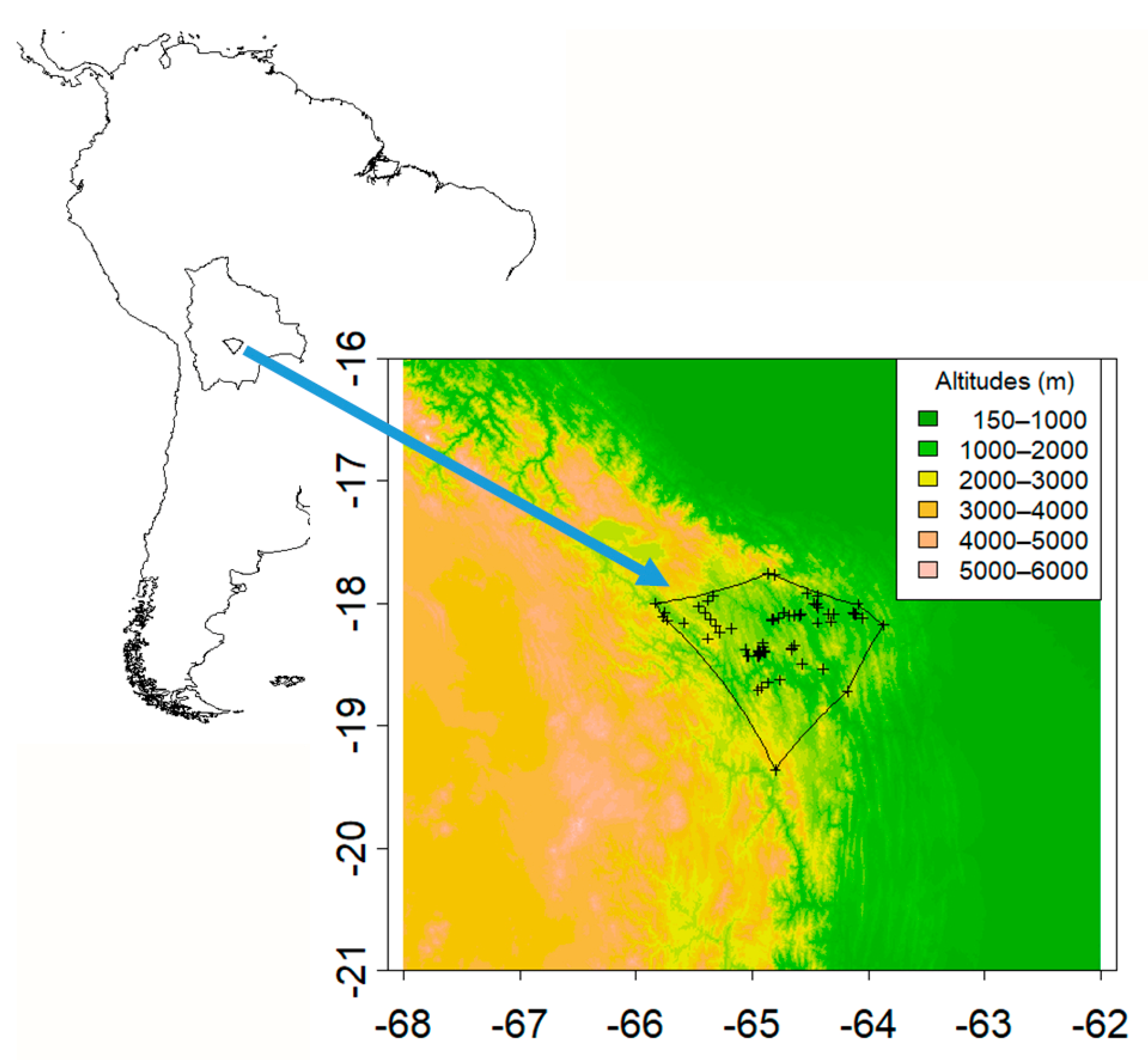
2.1. Species Occurrences
2.2. Climate Data
2.3. Dynamic Vegetation Modelling
2.4. A. rubrogenys and Plant Species SDM
3. Results
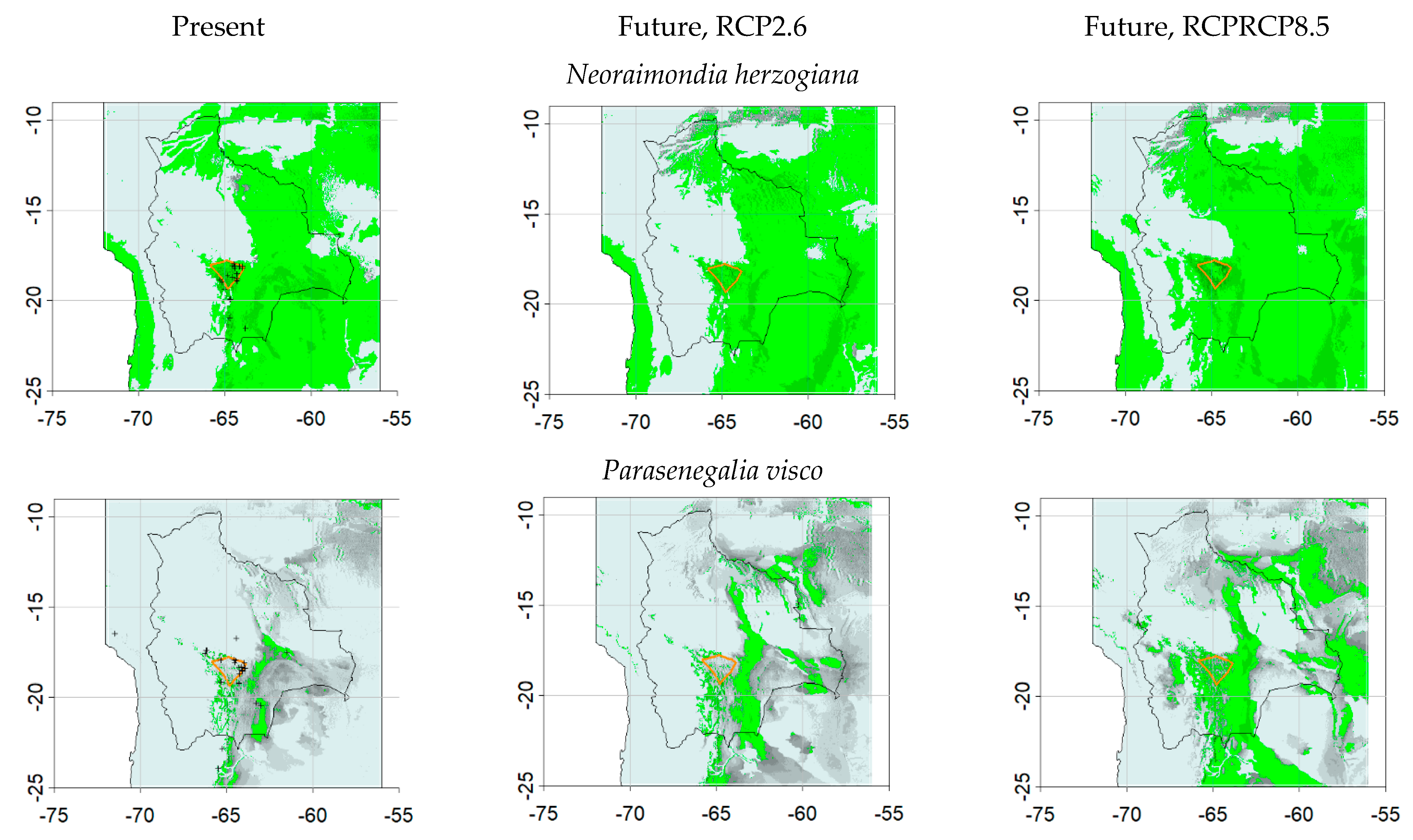
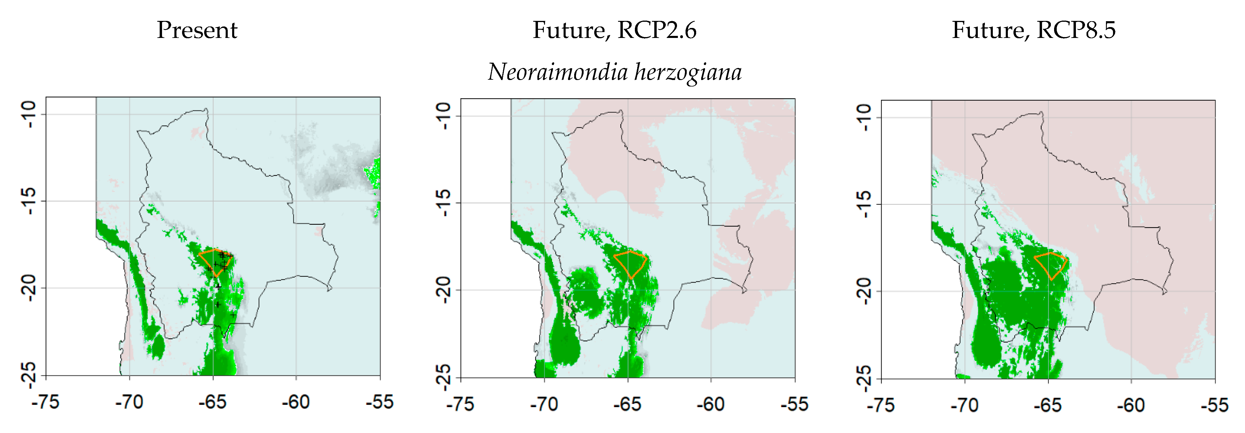
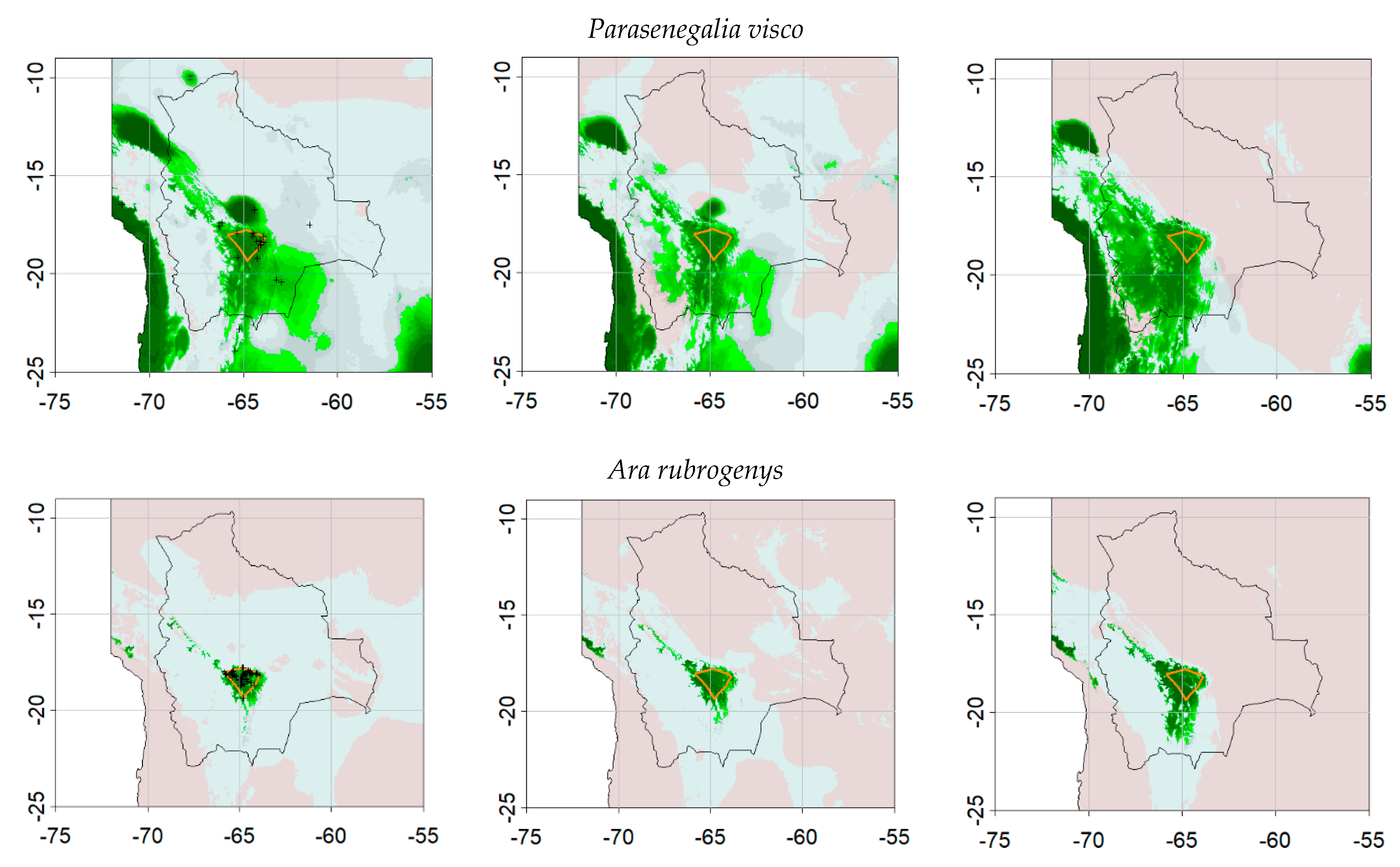
3.1. Dynamic Vegetation Modelling
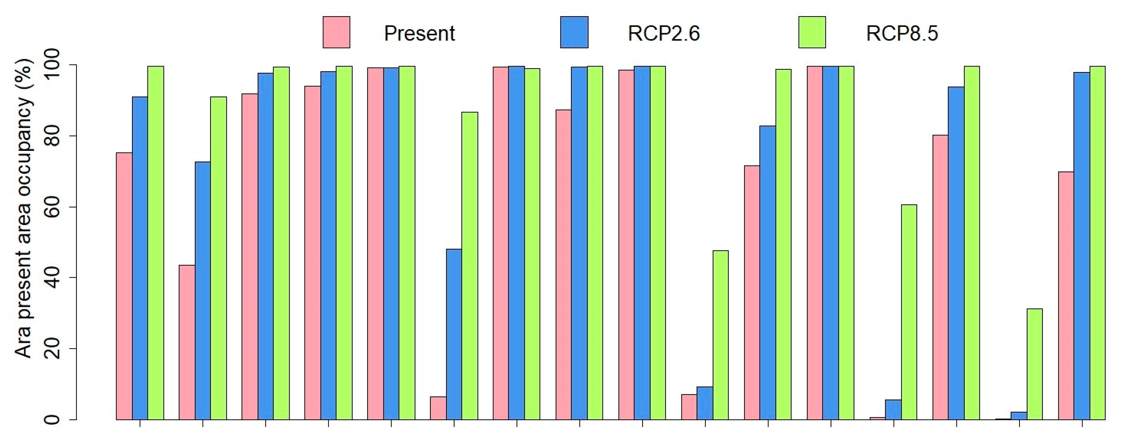
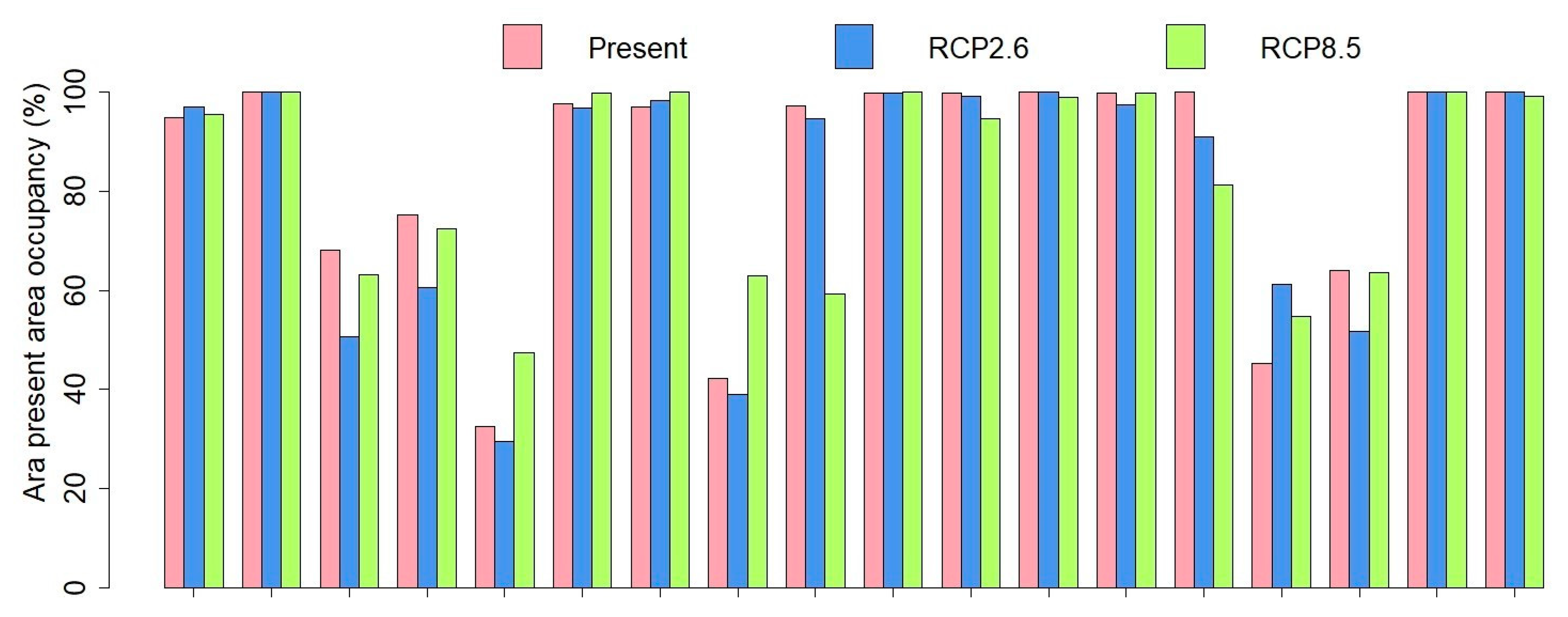
3.2. SDM Modelling
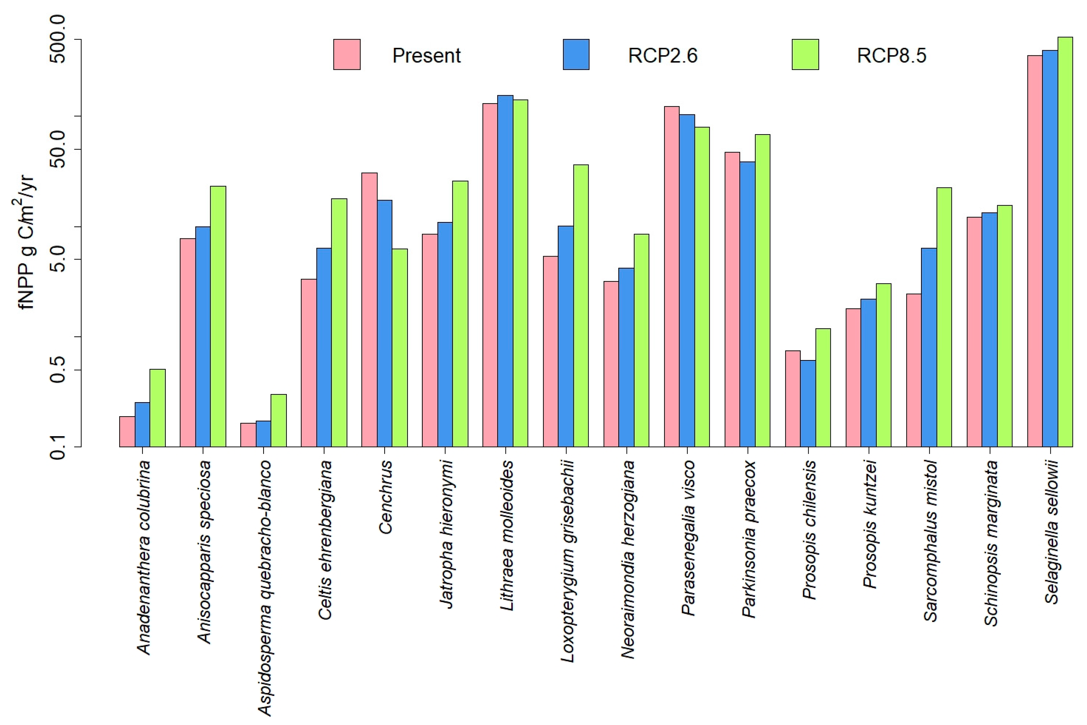
3.3. Comparisons of Plant Model Predictions for the Future
4. Discussion
5. Conclusions
Supplementary Materials
Author Contributions
Funding
Institutional Review Board Statement
Data Availability Statement
Acknowledgments
Conflicts of Interest
References
- Şekercioğlu Çağan, H.; Primack, R.B.; Wormworth, J. The effects of climate change on tropical birds. Biol. Conserv. 2012, 148, 1–18. [Google Scholar] [CrossRef]
- La Sorte, F.A.; Jetz, W. Tracking of climatic niche boundaries under recent climate change. J. Anim. Ecol. 2012, 81, 914–925. [Google Scholar] [CrossRef]
- Orme, C.D.L.; Davies, R.G.; Burgess, M.; Eigenbrod, F.; Pickup, N.; Olson, V.A.; Webster, A.J.; Ding, T.-S.; Rasmussen, P.C.; Ridgely, R.S.; et al. Global hotspots of species richness are not congruent with endemism or threat. Nat. Cell Biol. 2005, 436, 1016–1019. [Google Scholar] [CrossRef]
- Herzog, S.K.; Maillard, O.; Embert, D.; Caballero, P.; Quiroga, D. Range size estimates of Bolivian endemic bird species revisited: The importance of environmental data and national expert knowledge. J. Ornithol. 2012, 153, 1189–1202. [Google Scholar] [CrossRef]
- Lanning, D.V. Distribution and breeding biology of the Red-fronted Macaw. Wilson Bull. 1991, 103, 357–365. [Google Scholar]
- Tella, J.; Rojas, A.; Carrete, M.; Hiraldo, F. Simple assessments of age and spatial population structure can aid conservation of poorly known species. Biol. Conserv. 2013, 167, 425–434. [Google Scholar] [CrossRef]
- Herzog, S.K.; Kessler, M.; Maijer, S.; Hohnwald, S. Distributional notes on birds of Andean dry forests in Bolivia. Bull. Br. Ornithol. Club 1997, 117, 223–235. [Google Scholar]
- Boussekey, M.; Saint-Pie, J.; Morvan, O. Observations on a population of Red-fronted Macaws Ara rubrogenys in the Río Caine valley, central Bolivia. Bird Conserv. Int. 1991, 1, 335–350. [Google Scholar] [CrossRef] [Green Version]
- Pitter, E.; Christiansen, M.B. Ecology, status and conservation of the Red-fronted Macaw Ara rubrogenys. Bird Conserv. Int. 1995, 5, 61–78. [Google Scholar] [CrossRef] [Green Version]
- Herrera, M.; Hennessey, B. Quantifying the illegal parrot trade in Santa Cruz de la Sierra, Bolivia, with emphasis on threatened species. Bird Conserv. Int. 2007, 17, 295–300. [Google Scholar] [CrossRef] [Green Version]
- Rojas, A.; Zeballos, A.; Rocha, E.; Balderrama, J.A. Ara rubrogenys Lafrenaye 1847; Ministerio de Medio Ambiente y Agua: La Paz, Bolivia, 2009; pp. 332–334.
- BirdLife International. Ara rubrogenys. The IUCN Red List of Threatened Species. 2018. Available online: https://0-dx-doi-org.brum.beds.ac.uk/10.2305/IUCN.UK.2018-2.RLTS.T22685572A131382876.en (accessed on 21 September 2020).
- Rangecroft, S.; Harrison, S.; Anderson, K.; Magrath, J.; Castel, A.P.; Pacheco, P. Climate Change and Water Resources in Arid Mountains: An Example from the Bolivian Andes. Ambio 2013, 42, 852–863. [Google Scholar] [CrossRef] [Green Version]
- Botero-Delgadillo, E.; Páez, C.A.; Bayly, N. Biogeography and conservation of Andean and Trans-Andean populations of Pyrrhura parakeets in Colombia: Modelling geographic distributions to identify independent conservation units. Bird Conserv. Int. 2012, 22, 445–461. [Google Scholar] [CrossRef] [Green Version]
- Ferrer-Paris, J.R.; Sánchez-Mercado, A.; Rodríguez-Clark, K.M.; Rodríguez, J.P.; Rodríguez, G.A. Using limited data to detect changes in species distributions: Insights from Amazon parrots in Venezuela. Biol. Conserv. 2014, 173, 133–143. [Google Scholar] [CrossRef]
- Marini, M.Â.; Barbet-Massin, M.; Martinez, J.; Prestes, N.P.; Jiguet, F. Applying ecological niche modelling to plan conservation actions for the Red-spectacled Amazon (Amazona pretrei). Biol. Conserv. 2010, 143, 102–112. [Google Scholar] [CrossRef]
- Cardador, L.; Lattuada, M.; Strubbe, D.; Tella, J.L.; Reino, L.; Figueira, R.; Carrete, M. Regional Bans on Wild-Bird Trade Modify Invasion Risks at a Global Scale. Conserv. Lett. 2017, 10, 717–725. [Google Scholar] [CrossRef] [Green Version]
- López-López, P.; García-Ripollés, C.; Aguilar, J.M.; Garcia-López, F.; Verdejo, J. Modelling breeding habitat preferences of Bonelli’s eagle (Hieraaetus fasciatus) in relation to topography, disturbance, climate and land use at different spatial scales. J. Ornithol. 2005, 147, 97–106. [Google Scholar] [CrossRef]
- Preston, K.L.; Rotenberry, J.T.; Redak, R.A.; Allen, M.F. Habitat shifts of endangered species under altered climate conditions: Importance of biotic interactions. Glob. Chang. Biol. 2008, 14, 2501–2515. [Google Scholar] [CrossRef]
- Pidgeon, A.M.; Rivera, L.; Martinuzzi, S.; Politi, N.; Bateman, B.L. Will representation targets based on area protect critical resources for the conservation of the Tucuman Parrot? Condor 2015, 117, 503–517. [Google Scholar] [CrossRef] [Green Version]
- Fitter, A.; Hay, R. Environmental Physiology of Plants; Elsevier: Amsterdam, The Netherlands, 2002; p. 367. [Google Scholar]
- Smith, N.G.; Dukes, J.S. Plant respiration and photosynthesis in global-scale models: Incorporating acclimation to temperature and CO. Glob. Chang. Biol. 2012, 19, 45–63. [Google Scholar] [CrossRef]
- Dury, M.; Hambuckers, A.; Warnant, P.; Henrot, A.; Favre, E.; Ouberdous, M.; François, L. Responses of European forest ecosystems to 21st century climate: Assessing changes in interannual variability and fire intensity. iForest Biogeosci. For. 2011, 4, 82–99. [Google Scholar] [CrossRef]
- Raghunathan, N.; François, L.; Huynen, M.-C.; Oliveira, L.C.; Hambuckers, A. Modelling the distribution of key tree species used by lion tamarins in the Brazilian Atlantic forest under a scenario of future climate change. Reg. Environ. Chang. 2014, 15, 683–693. [Google Scholar] [CrossRef]
- Blanco, G.; Hiraldo, F.; Rojas, A.; Dénes, F.V.; Tella, J.L. Parrots as key multilinkers in ecosystem structure and functioning. Ecol. Evol. 2015, 5, 4141–4160. [Google Scholar] [CrossRef] [Green Version]
- Montesinos-Navarro, A.; Hiraldo, F.; Tella, J.L.; Blanco, G. Network structure embracing mutualism–antagonism continuums increases community robustness. Nat. Ecol. Evol. 2017, 1, 1661–1669. [Google Scholar] [CrossRef]
- Burgman, M.A.; Fox, J.C. Bias in species range estimates from minimum convex polygons: Implications for conservation and options for improved planning. Anim. Conserv. 2003, 6, 19–28. [Google Scholar] [CrossRef] [Green Version]
- Pateiro-López, B.; Rodríguez-Casal, A. Generalizing the Convex Hull of a Sample: TheRPackagealphahull. J. Stat. Softw. 2010, 34, 1–28. [Google Scholar] [CrossRef] [Green Version]
- Fick, S.E.; Hijmans, R.J. WorldClim 2: New 1-km spatial resolution climate surfaces for global land areas. Int. J. Climatol. 2017, 37, 4302–4315. [Google Scholar] [CrossRef]
- The HadGEM2 Development Team; Martin, G.M.; Bellouin, N.; Collins, W.J.; Culverwell, I.D.; Halloran, P.R.; Hardiman, S.C.; Hinton, T.J.; Jones, C.D.; McDonald, R.E.; et al. The HadGEM2 family of Met Office Unified Model climate configurations. Geosci. Model Dev. 2011, 4, 723–757. [Google Scholar] [CrossRef] [Green Version]
- Moss, R.H.; Edmonds, J.A.; Hibbard, K.A.; Manning, M.R.; Rose, S.K.; Van Vuuren, D.P.; Carter, T.R.; Emori, S.; Kainuma, M.; Kram, T.; et al. The next generation of scenarios for climate change research and assessment. Nature 2010, 463, 747–756. [Google Scholar] [CrossRef] [PubMed]
- Stocker, T.F.; Qin, D.; Plattner, G.-K.; Tignor, M.; Allen, S.K.; Boschung, J.; Nauels, A.; Xia, Y.; Bex, V.; Midgley, P.M. Climate Change 2013: The Physical Science Basis; Working Group I Contribution to the Fifth Assessment Report of the Intergovernmental Panel on Climate Change; Cambridge University Press: Cambridge, UK; New York, NY, USA, 2013. [Google Scholar] [CrossRef] [Green Version]
- Warnant, P.; François, L.; Strivay, D.; Gérard, J.-C. CARAIB: A global model of terrestrial biological productivity. Glob. Biogeochem. Cycles 1994, 8, 255–270. [Google Scholar] [CrossRef]
- Gérard, J.C.; Nemry, B.; François, L.M.; Warnant, P. The interannual change of atmospheric CO2: Contribution of subtropical ecosystems? Geophys. Res. Lett. 1999, 26, 243–246. [Google Scholar] [CrossRef]
- Otto, D.; Rasse, D.; Kaplan, J.; Warnant, P.; François, L. Biospheric carbon stocks reconstructed at the Last Glacial Maximum: Comparison between general circulation models using prescribed and computed sea surface temperatures. Glob. Planet. Chang. 2002, 33, 117–138. [Google Scholar] [CrossRef]
- Laurent, J.; Francois, L.; Barhen, A.; Bel, L.; Cheddadi, R. European bioclimatic affinity groups: Data-model comparisons. Glob. Planet. Chang. 2008, 61, 28–40. [Google Scholar] [CrossRef]
- François, L.; Goddéris, Y.; Munhoven, G. Modelling the interactions between biospheric and weathering processes: Towards a mechanistic description of the land environment. Mineral. Mag. 1998, 62A, 468–469. [Google Scholar] [CrossRef]
- François, L.M.; Goddéris, Y.; Warnant, P.; Ramstein, G.; De Noblet, N.; Lorenz, S. Carbon stocks and isotopic budgets of the terrestrial biosphere at mid-Holocene and last glacial maximum times. Chem. Geol. 1999, 159, 163–189. [Google Scholar] [CrossRef]
- François, L.; Ghislain, M.; Otto, D.; Micheels, A. Late Miocene vegetation reconstruction with the CARAIB model. Palaeogeogr. Palaeoclim. Palaeoecol. 2006, 238, 302–320. [Google Scholar] [CrossRef] [Green Version]
- François, L.; Utescher, T.; Favre, E.; Henrot, A.-J.; Warnant, P.; Micheels, A.; Erdei, B.; Suc, J.-P.; Cheddadi, R.; Mosbrugger, V. Modelling Late Miocene vegetation in Europe: Results of the CARAIB model and comparison with palaeovegetation data. Palaeogeogr. Palaeoclim. Palaeoecol. 2011, 304, 359–378. [Google Scholar] [CrossRef]
- Henrot, A.-J.; François, L.; Favre, E.; Butzin, M.; Ouberdous, M.; Munhoven, G. Effects of CO2, continental distribution, topography and vegetation changes on the climate at the Middle Miocene: A model study. Clim. Past 2010, 6, 675–694. [Google Scholar] [CrossRef] [Green Version]
- Henrot, A.-J.; Utescher, T.; Erdei, B.; Dury, M.; Hamon, N.; Ramstein, G.; Krapp, M.; Herold, N.; Goldner, A.; Favre, E.; et al. Middle Miocene climate and vegetation models and their validation with proxy data. Palaeogeogr. Palaeoclim. Palaeoecol. 2017, 467, 95–119. [Google Scholar] [CrossRef]
- Chang, J.; Ciais, P.; Wang, X.; Piao, S.; Asrar, G.; Betts, R.; Chevallier, F.; Dury, M.; François, L.; Frieler, K.; et al. Benchmarking carbon fluxes of the ISIMIP2a biome models. Environ. Res. Lett. 2017, 12, 045002. [Google Scholar] [CrossRef] [Green Version]
- Fontaine, C.M.; Dendoncker, N.; De Vreese, R.; Jacquemin, I.; Marek, A.; Van Herzeleg, A.; Devillet, G.; Mortelmans, D.; François, L. Towards participatory integrated valuation and modelling of ecosystem services under land-use change. J. Land Use Sci. 2014, 9, 278–303. [Google Scholar] [CrossRef]
- Minet, J.; Laloy, E.; Tychon, B.; Francois, L. Bayesian inversions of a dynamic vegetation model at four European grassland sites. Biogeosciences 2015, 12, 2809–2829. [Google Scholar] [CrossRef] [Green Version]
- Fronzek, S.; Pirttioja, N.; Carter, T.R.; Bindi, M.; Hoffmann, H.; Palosuo, T.; Ruiz-Ramos, M.; Tao, F.; Trnka, M.; Acutis, M.; et al. Classifying multi-model wheat yield impact response surfaces showing sensitivity to temperature and precipitation change. Agric. Syst. 2018, 159, 209–224. [Google Scholar] [CrossRef]
- Cheddadi, R.; Henrot, A.-J.; François, L.; Boyer, F.; Bush, M.; Carré, M.; Coissac, E.; De Oliveira, P.E.; Ficetola, F.; Hambuckers, A.; et al. Microrefugia, Climate Change, and Conservation of Cedrus atlantica in the Rif Mountains, Morocco. Front. Ecol. Evol. 2017, 5. [Google Scholar] [CrossRef] [Green Version]
- Dury, M.; Mertens, L.; Fayolle, A.; Verbeeck, H.; Hambuckers, A.; François, L. Refining Species Traits in a Dynamic Vegetation Model to Project the Impacts of Climate Change on Tropical Trees in Central Africa. Forests 2018, 9, 722. [Google Scholar] [CrossRef] [Green Version]
- Raghunathan, N.; François, L.; Dury, M.; Hambuckers, A. Contrasting climate risks predicted by dynamic vegetation and ecological niche-based models applied to tree species in the Brazilian Atlantic Forest. Reg. Environ. Chang. 2018, 19, 219–232. [Google Scholar] [CrossRef]
- Allouche, O.; Tsoar, A.; Kadmon, R. Assessing the accuracy of species distribution models: Prevalence, kappa and the true skill statistic (TSS). J. Appl. Ecol. 2006, 43, 1223–1232. [Google Scholar] [CrossRef]
- Segurado, P.; Araújo, M.B. An evaluation of methods for modelling species distributions. J. Biogeogr. 2004, 31, 1555–1568. [Google Scholar] [CrossRef]
- Meynard, C.N.; Quinn, J.F. Predicting species distributions: A critical comparison of the most common statistical models using artificial species. J. Biogeogr. 2007, 34, 1455–1469. [Google Scholar] [CrossRef]
- Bedia, J.; Busqué, J.; Gutiérrez, J.M. Predicting plant species distribution across an alpine rangeland in northern Spain. A comparison of probabilistic methods. Appl. Veg. Sci. 2011, 14, 415–432. [Google Scholar] [CrossRef] [Green Version]
- King, G.; Zeng, L.; Tomz, M. Logistic Regression in Rare Events Data. J. Stat. Softw. 2003, 8, 1–27. [Google Scholar] [CrossRef]
- Elith, J.; Graham, C.H.; Anderson, R.P.; Dudík, M.; Ferrier, S.; Guisan, A.; Hijmans, R.J.; Huettmann, F.; Leathwick, J.R.; Lehmann, A.; et al. Novel methods improve prediction of species’ distributions from occurrence data. Ecography 2006, 29, 129–151. [Google Scholar] [CrossRef] [Green Version]
- Calcagno, V.; De Mazancourt, C. glmulti: AnRPackage for Easy Automated Model Selection with (Generalized) Linear Models. J. Stat. Softw. 2010, 34, 1–29. [Google Scholar] [CrossRef] [Green Version]
- Vanderwal, J.; Shoo, L.P.; Graham, C.; Williams, S.E. Selecting pseudo-absence data for presence-only distribution modeling: How far should you stray from what you know? Ecol. Model. 2009, 220, 589–594. [Google Scholar] [CrossRef]
- VanDerWal, J.; Lorena Falconi, L.; Januchowski, S.; Shoo, L.; Storlie, C. Species Distribution Modelling Tools: Tools for Pro-Cessing Data Associated with Species Distribution Modelling Exercises. 2014. Available online: https://www.rforge.net/SDMTools/ (accessed on 26 November 2020).
- Dormann, C.F.; Elith, J.; Bacher, S.; Buchmann, C.; Carl, G.; Carré, G.; Marquéz, J.R.G.; Gruber, B.; Lafourcade, B.; Leitão, P.J.; et al. Collinearity: A review of methods to deal with it and a simulation study evaluating their performance. Ecography 2012, 36, 27–46. [Google Scholar] [CrossRef]
- Bolliger, J.; Kienast, F.; Bugmann, H. Comparing models for tree distributions: Concept, structures, and behavior. Ecol. Model. 2000, 134, 89–102. [Google Scholar] [CrossRef]
- Morin, X.; Thuiller, W. Comparing niche- and process-based models to reduce prediction uncertainty in species range shifts under climate change. Ecolology 2009, 90, 1301–1313. [Google Scholar] [CrossRef]
- Cheaib, A.; Badeau, V.; Boe, J.; Chuine, I.; Delire, C.; Dufrêne, E.; François, C.; Gritti, E.S.; Legay, M.; Pagé, C.; et al. Climate change impacts on tree ranges: Model intercomparison facilitates understanding and quantification of uncertainty. Ecol. Lett. 2012, 15, 533–544. [Google Scholar] [CrossRef]
- Takolander, A.; Hickler, T.; Meller, L.; Cabeza, M. Comparing future shifts in tree species distributions across Europe projected by statistical and dynamic process-based models. Reg. Environ. Chang. 2018, 19, 251–266. [Google Scholar] [CrossRef] [Green Version]
- Ramirez-Villegas, J.; Cuesta, F.; Devenish, C.; Peralvo, M.; Jarvis, A.; Arnillas, C.A. Using species distributions models for designing conservation strategies of Tropical Andean biodiversity under climate change. J. Nat. Conserv. 2014, 22, 391–404. [Google Scholar] [CrossRef] [Green Version]
- Fadrique, B.; Báez, S.; Duque, Á.; Malizia, A.; Blundo, C.; Carilla, J.; Osinaga-Acosta, O.; Malizia, L.; Silman, M.; Farfán-Ríos, W.; et al. Widespread but heterogeneous responses of Andean forests to climate change. Nat. Cell Biol. 2018, 564, 207–212. [Google Scholar] [CrossRef]
- Steinbauer, M.J.; Grytnes, J.-A.; Jurasinski, G.; Kulonen, A.; Lenoir, J.; Pauli, H.; Rixen, C.; Winkler, M.; Bardy-Durchhalter, M.; Barni, E.; et al. Accelerated increase in plant species richness on mountain summits is linked to warming. Nat. Cell Biol. 2018, 556, 231–234. [Google Scholar] [CrossRef]
- Heinrich, B. Why Have Some Animals Evolved to Regulate a High Body Temperature? Am. Nat. 1977, 111, 623–640. [Google Scholar] [CrossRef]
- McKechnie, A.E.; Wolf, B.O. Climate change increases the likelihood of catastrophic avian mortality events during extreme heat waves. Biol. Lett. 2009, 6, 253–256. [Google Scholar] [CrossRef] [Green Version]
- Tingley, M.W.; Monahan, W.B.; Beissinger, S.R.; Moritz, C. Birds track their Grinnellian niche through a century of climate change. Proc. Natl. Acad. Sci. USA 2009, 106, 19637–19643. [Google Scholar] [CrossRef] [Green Version]
- Avalos, V.D.R.; Hernández, J. Projected distribution shifts and protected area coverage of range-restricted Andean birds under climate change. Glob. Ecol. Conserv. 2015, 4, 459–469. [Google Scholar] [CrossRef]
- Williams, S.; Williams, Y.M.; Vanderwal, J.; Isaac, J.L.; Shoo, L.P.; Johnson, C.N. Ecological specialization and population size in a biodiversity hotspot: How rare species avoid extinction. Proc. Natl. Acad. Sci. USA 2009, 106, 19737–19741. [Google Scholar] [CrossRef] [PubMed] [Green Version]
- Early, R.; Sax, D.F. Climatic niche shifts between species’ native and naturalized ranges raise concern for ecological forecasts during invasions and climate change. Glob. Ecol. Biogeogr. 2014, 23, 1356–1365. [Google Scholar] [CrossRef]
- Bocsi, T.; Allen, J.M.; Bellemare, J.; Kartesz, J.; Nishino, M.; Bradley, B.A. Plants’ native distributions do not reflect climatic tolerance. Divers. Distrib. 2016, 22, 615–624. [Google Scholar] [CrossRef] [Green Version]
- Abellán, P.; Tella, J.L.; Carrete, M.; Cardador, L.; Anadón, J.D. Climate matching drives spread rate but not establishment success in recent unintentional bird introductions. Proc. Natl. Acad. Sci. USA 2017, 114, 9385–9390. [Google Scholar] [CrossRef] [Green Version]
- Hartig, F.; Dyke, J.G.; Hickler, T.; Higgins, S.I.; O’Hara, R.B.; Scheiter, S.; Huth, A. Connecting dynamic vegetation models to data—An inverse perspective. J. Biogeogr. 2012, 39, 2240–2252. [Google Scholar] [CrossRef]
- Bloomfield, K.J.; Cernusak, L.A.; Eamus, D.; Ellsworth, D.S.; Prentice, I.C.; Wright, I.J.; Boer, M.M.; Bradford, M.G.; Cale, P.; Cleverly, J.; et al. A continental-scale assessment of variability in leaf traits: Within species, across sites and between seasons. Funct. Ecol. 2018, 32, 1492–1506. [Google Scholar] [CrossRef]
- Gillison, A.N. Plant functional indicators of vegetation response to climate change, past present and future: I. Trends, emerging hypotheses and plant functional modality. Flora Morphol. Distrib. Funct. Ecol. Plants 2019, 254, 12–30. [Google Scholar] [CrossRef]
- Modeling past plant species’ distributions in mountainous areas: A way to improve our knowledge of future climate change impacts? Past Glob. Chang. Mag. 2020, 28, 16–17. [CrossRef]
- Kattge, J.; Bönisch, G.; Díaz, S.; Lavorel, S.; Prentice, I.C.; Leadley, P.; Tautenhahn, S.; Werner, G.D.A.; Aakala, T.; Abedi, M.; et al. TRY plant trait database – enhanced coverage and open access. Glob. Chang. Biol. 2019, 26, 119–188. [Google Scholar] [CrossRef] [Green Version]
- Rojas, A.; Yucra, E.; Vera, I.; Requejo, A.; Tella, J. A new population of the globally Endangered Red-fronted Macaw Ara rubrogenys unusually breeding in palms. Bird Conserv. Int. 2012, 24, 389–392. [Google Scholar] [CrossRef] [Green Version]
- Blanco, G.; Morinha, F.; Roques, S.; Hiraldo, F.; Rojas, A.; Tella, J.L. Fine-scale genetic structure in the critically endangered red-fronted macaw in the absence of geographic and ecological barriers. Sci. Rep. 2021, 11, 1–17. [Google Scholar] [CrossRef] [PubMed]
- Spooner, F.E.B.; Pearson, R.G.; Freeman, R. Rapid warming is associated with population decline among terrestrial birds and mammals globally. Glob. Chang. Biol. 2018, 24, 4521–4531. [Google Scholar] [CrossRef] [Green Version]


| Species | Occurrences | Sources |
|---|---|---|
| Anadenanthera colubrina | 3272 | GBIF.org (12 August 2020) GBIF Occurrence Download https://0-doi-org.brum.beds.ac.uk/10.15468/dl.xccvu7 |
| Anisocapparis speciosa | 218 | GBIF.org (12 August 2020) GBIF Occurrence Download https://0-doi-org.brum.beds.ac.uk/10.15468/dl.xxw4c9 |
| Ara rubrogenys | 159 | This study |
| Aspidosperma quebracho-blanco | 394 | GBIF.org (12 August 2020) GBIF Occurrence Download https://0-doi-org.brum.beds.ac.uk/10.15468/dl.xccvu7 |
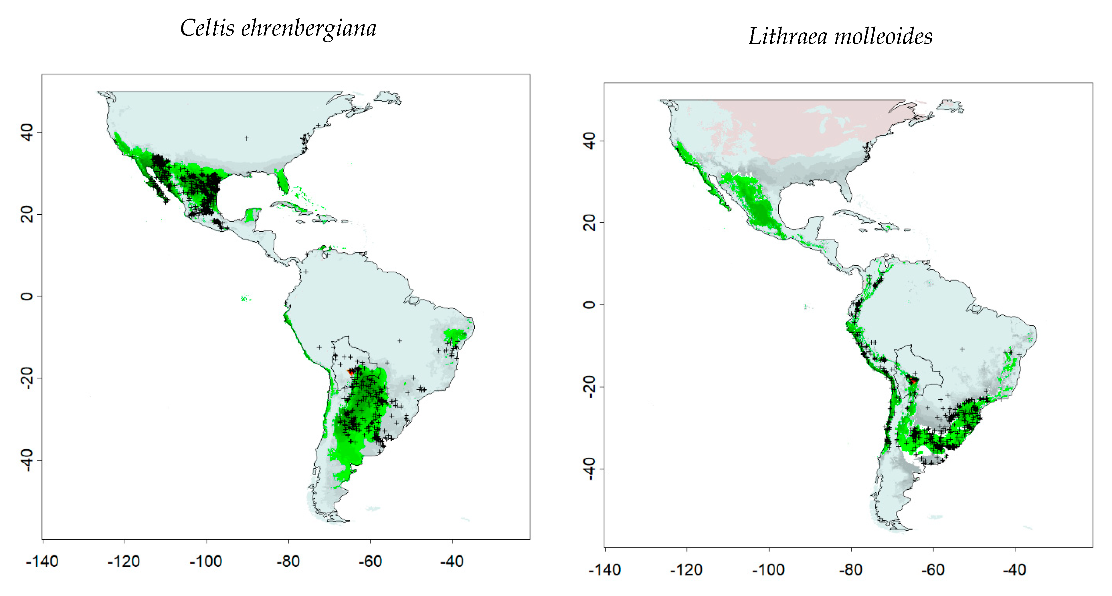
| Celtis ehrenbergiana | 2528 | GBIF.org (11 August 2020) GBIF Occurrence Download https://0-doi-org.brum.beds.ac.uk/10.15468/dl.ph4g3s |
| Cenchrus | 8069 | GBIF.org (12 August 2020) GBIF Occurrence Download https://0-doi-org.brum.beds.ac.uk/10.15468/dl.3s3af9 |
| Cnidoscolus tubulosus. | 159 | GBIF.org (6 January 2017) GBIF Occurrence Download http://0-doi-org.brum.beds.ac.uk/10.15468/dl.wwofy0 |
| Jatropha hieronymi | 96 | GBIF.org (6 January 2017) GBIF Occurrence Download http://0-doi-org.brum.beds.ac.uk/10.15468/dl.2ziu73, |
| Lithraea molleoides | 13,271 | GBIF.org (12 August 2020) GBIF Occurrence Download https://0-doi-org.brum.beds.ac.uk/10.15468/dl.m45p2c |
| Loxopterygium grisebachii | 86 | GBIF.org (11 August 2020) GBIF Occurrence Download https://0-doi-org.brum.beds.ac.uk/10.15468/dl.3zkvc4 |
| Neoraimondia herzogiana | 29 | GBIF.org (12 August 2020) GBIF Occurrence Download https://0-doi-org.brum.beds.ac.uk/10.15468/dl.xag67z |
| Parasenegalia visco | 34 | GBIF.org (12 August 2020) GBIF Occurrence Download https://0-doi-org.brum.beds.ac.uk/10.15468/dl.mnw4qm |
| Parkinsonia praecox | 1123 | GBIF.org (12 August 2020) GBIF Occurrence Download https://0-doi-org.brum.beds.ac.uk/10.15468/dl.fk3as9 |
| Prosopis chilensis | 81 | GBIF.org (6 January 2017) GBIF Occurrence Download http://0-doi-org.brum.beds.ac.uk/10.15468/dl.dh9ski |
| Prosopis kuntzei Kuntze | 68 | GBIF.org (6 January 2017) GBIF Occurrence Download http://0-doi-org.brum.beds.ac.uk/10.15468/dl.dh9ski |
| Sarcomphalus mistol | 217 | GBIF.org (11 August 2020) GBIF Occurrence Download https://0-doi-org.brum.beds.ac.uk/10.15468/dl.mk3r74 |
| Schinopsis marginata Engl. | 41 | GBIF.org (6 January 2017) GBIF Occurrence Download http://0-doi-org.brum.beds.ac.uk/10.15468/dl.ngmuf4 |
| Selaginella sellowii | 924 | GBIF.org (21 August 2020) GBIF Occurrence Download https://0-doi-org.brum.beds.ac.uk/10.15468/dl.5d5hwt |
| Plant Species | N | AUC | TSS | Threshold | Max fNPP | Se | Sp |
|---|---|---|---|---|---|---|---|
| Anadenanthera colubrina | 1643 | 0.67569 | 0.41083 | 0.0015 | 318.03 | 0.9434 | 0.46744 |
| Anisocapparis speciosa | 147 | 0.60454 | 0.40816 | 4.5738 | 1131.69 | 0.95918 | 0.44898 |
| Aspidosperma quebracho-blanco | 218 | 0.6508 | 0.38991 | 0.0706 | 1064.81 | 0.94495 | 0.44495 |
| Celtis ehrenbergiana | 1444 | 0.63466 | 0.47715 | 0.1982 | 1253.74 | 0.96676 | 0.51039 |
| Cenchrus | 4449 | 0.66834 | 0.35042 | 0.4236 | 930.89 | 0.82513 | 0.52529 |
| Cnidoscolus tubulosus | 145 | 0.68628 | 0.4 | 19.5846 | 1071.89 | 0.76552 | 0.63448 |
| Jatropha hieronymi | 54 | 0.73131 | 0.61111 | 7.0216 | 1049.12 | 0.92593 | 0.68519 |
| Lithraea molleoides | 1870 | 0.75729 | 0.61176 | 0.3059 | 1184.87 | 0.94759 | 0.66417 |
| Loxopterygium grisebachii | 49 | 0.75052 | 0.57143 | 1.6223 | 1112.63 | 0.91837 | 0.65306 |
| Neoraimondia herzogiana | 25 | 0.4784 | 0.4 | 0.0053 | 1111.65 | 0.9600 | 0.4400 |
| Parasenegalia visco | 29 | 0.6629 | 0.44828 | 47.2607 | 1417.99 | 0.7931 | 0.65517 |
| Parkinsonia praecox | 550 | 0.53771 | 0.38 | 12.7344 | 851.75 | 0.95818 | 0.42182 |
| Prosopis chilensis | 76 | 0.47152 | 0.17105 | 0.0238 | 1067.33 | 0.89474 | 0.27632 |
| Prosopis kuntzei | 67 | 0.62364 | 0.44776 | 1.4721 | 1009.61 | 0.91045 | 0.53731 |
| Sarcomphalus mistol | 149 | 0.63799 | 0.41611 | 0.7605 | 1206.76 | 0.95973 | 0.45638 |
| Schinopsis marginata | 38 | 0.76939 | 0.57895 | 10.2059 | 1246.94 | 0.81579 | 0.76316 |
| Selaginella sellowii | 277 | 0.72557 | 0.38628 | 274.332 | 910.91 | 0.66065 | 0.72563 |
| Species | N | D | AUC | TSS | Thresh. | Se | Sp |
|---|---|---|---|---|---|---|---|
| Ara rubrogenys | 367 | 320 | 0.9775 | 0.943 | 0.2756 | 0.9623 | 0.9557 |
| Anadenanthera colubrina | 8173 | 1800 | 0.8584 | 0.6016 | 0.1685 | 0.7823 | 0.7830 |
| Anisocapparis speciosa | 583 | 1800 | 0.9445 | 0.7987 | 0.2124 | 0.8776 | 0.8807 |
| Aspidosperma quebracho-blanco | 1018 | 1800 | 0.9195 | 0.733 | 0.2113 | 0.8609 | 0.8591 |
| Celtis ehrenbergiana | 6495 | 1800 | 0.9008 | 0.6889 | 0.2363 | 0.8322 | 0.8322 |
| Cenchrus | 20,713 | 2000 | 0.7794 | 0.4257 | 0.2040 | 0.6982 | 0.6974 |
| Cnidoscolus tubulosus | 463 | 1400 | 0.8143 | 0.4527 | 0.3983 | 0.7172 | 0.7179 |
| Jatropha hieronymi | 246 | 1200 | 0.9292 | 0.7876 | 0.2605 | 0.8889 | 0.8802 |
| Lithraea molleoides | 4758 | 1600 | 0.9338 | 0.7401 | 0.5555 | 0.8698 | 0.8696 |
| Loxopterygium grisebachii | 221 | 1800 | 0.9762 | 0.872 | 0.2044 | 0.9388 | 0.9302 |
| Neoraimondia herzogiana | 83 | 1400 | 0.9903 | 0.9483 | 0.3278 | 0.9600 | 0.9655 |
| Parasenegalia visco | 97 | 800 | 0.9113 | 0.6805 | 0.2914 | 0.8276 | 0.8235 |
| Parkinsonia praecox | 2807 | 1800 | 0.9203 | 0.6987 | 0.1788 | 0.8419 | 0.8418 |
| Prosopis chilensis | 238 | 2000 | 0.8530 | 0.694 | 0.4665 | 0.8421 | 0.8395 |
| Prosopis kuntzei | 203 | 1800 | 0.9231 | 0.7857 | 0.3598 | 0.8955 | 0.8897 |
| Sarcomphalus mistol | 583 | 1600 | 0.9367 | 0.7763 | 0.2489 | 0.8800 | 0.8799 |
| Schinopsis marginata | 120 | 1400 | 0.9570 | 0.8723 | 0.3762 | 0.9211 | 0.9268 |
| Selaginella sellowii | 1071 | 1400 | 0.7794 | 0.6669 | 0.3496 | 0.8267 | 0.8262 |
Publisher’s Note: MDPI stays neutral with regard to jurisdictional claims in published maps and institutional affiliations. |
© 2021 by the authors. Licensee MDPI, Basel, Switzerland. This article is an open access article distributed under the terms and conditions of the Creative Commons Attribution (CC BY) license (http://creativecommons.org/licenses/by/4.0/).
Share and Cite
Hambuckers, A.; de Harenne, S.; Rocha Ledezma, E.; Zúñiga Zeballos, L.; François, L. Predicting the Future Distribution of Ara rubrogenys, an Endemic Endangered Bird Species of the Andes, Taking into Account Trophic Interactions. Diversity 2021, 13, 94. https://0-doi-org.brum.beds.ac.uk/10.3390/d13020094
Hambuckers A, de Harenne S, Rocha Ledezma E, Zúñiga Zeballos L, François L. Predicting the Future Distribution of Ara rubrogenys, an Endemic Endangered Bird Species of the Andes, Taking into Account Trophic Interactions. Diversity. 2021; 13(2):94. https://0-doi-org.brum.beds.ac.uk/10.3390/d13020094
Chicago/Turabian StyleHambuckers, Alain, Simon de Harenne, Eberth Rocha Ledezma, Lilian Zúñiga Zeballos, and Louis François. 2021. "Predicting the Future Distribution of Ara rubrogenys, an Endemic Endangered Bird Species of the Andes, Taking into Account Trophic Interactions" Diversity 13, no. 2: 94. https://0-doi-org.brum.beds.ac.uk/10.3390/d13020094